The document serves as a mathematics primer aimed at refreshing essential topics such as calculus, linear algebra, differential equations, and probability & statistics. It defines fundamental mathematical concepts and functions, emphasizing functions' roles in mapping domains to ranges, along with discussions on various types of functions and their properties. Additionally, the document covers limits, exponential and logarithmic functions, and trigonometric functions, illustrating mathematical behaviors and identities.

1. GLOBAL STANDARD IN FINANCIAL ENGINEERING
CERTIFICATE IN
FINANCE
CQF
Certificate in Quantitative Finance
Subtext to go here
PowerPoint cover landscape2.indd 1 21/10/2011 10:53
June 2012
Maths Primer
This is a revision course designed to act as a mathematics refresher. The
volume of work covered is signi…cantly large so the emphasis is on working
through the notes and problem sheets. The four topics covered are
Calculus
Linear Algebra
Di¤erential Equations
Probability & Statistics
Page 1
1 Introduction to Calculus
1.1 Basic Terminology
We begin by de…ning some mathematical shorthand and number systems
9 there exists
8 for all
) therefore
* because
! which gives
s.t such that
: such that
i¤ if and only if
equivalent
similar
2 an element of
!x a unique x
Page 2
Natural Numbers N = f0; 1; 2; 3; :::::g
Integers ( N) Z = f0; 1; 2; 3; :::::g
Rationals p
q : p; q 2 Z; Q =
n
1
2; 0:76; 2:25; 0:3333333::::
o
Irrationals Q =
np
2; 0:01001000100001:::; ; e
o
Reals R all the above
Complex C =
n
x + iy : i =
p
1
o
Page 3

2. (a; b) = a < x < b open interval
[a; b] = a x b closed interval
(a; b] = a < x b semi-open/closed interval
[a; b) = a x < b semi-open/closed interval
So typically we would write x 2 (a; b) :
Examples
1 < x < 1 ( 1; 1)
1 < x b ( 1; b]
a x < 1 [a; 1)
Page 4
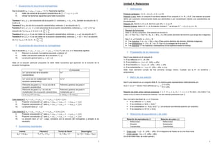
1.2 Functions
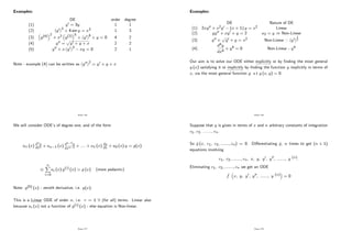
This is a term we use very loosely, but what is a function? Clearly it is a type of
black box with some input and a corresponding output. As long as the correct
result comes out we usually are not too concerned with what happens ’
inside’
.
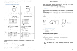
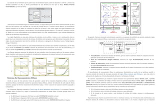
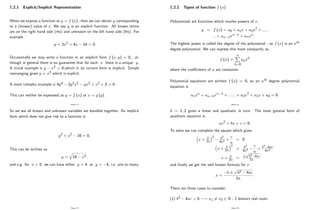
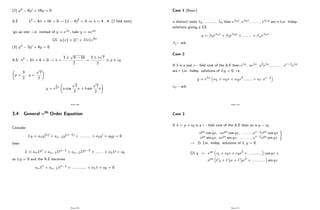
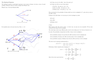
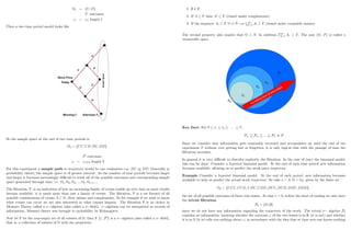
A function denoted f (x) of a single variable x is a rule that assigns each ele-
ment of a set X (written x 2 X) to exactly one element y of a set Y (y 2 Y ) :
A function is denoted by the form y = f (x) or x 7! f (x) :
We can also write f : X ! Y; which is saying that f is a mapping such that
all members of the input set X are mapped to elements of the output set Y:
So clearly there are a number of ways to describe the workings of a function.
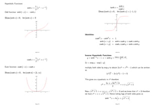
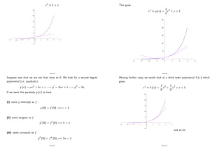
For example, if f (x) = x3; then f ( 2) = 23 = 8:
Page 5
-30
-20
-10
0
10
20
30
-4 -3 -2 -1 0 1 2 3 4
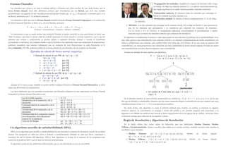
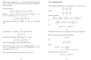
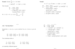
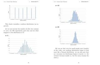
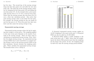
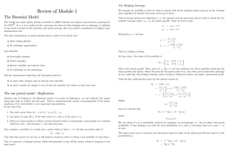
We often write y = f (x) where y is the dependent variable and x is the
independent variable.
Page 6
The set X is called the domain of f and the set Y is called the image (or
range), written Domf and Im f; in turn. For a given value of x there should
be at most one value of y. So the role of a function is to operate on the
domain and map it across uniquely to the range.
So we have seen two notations for the same operation.
The …rst y = f (x) suggests a graphical representation whilst the second
f : X ! Y establishes the idea of a mapping.
Page 7

3. There are three types of mapping:
1. For each x 2 X; 9 one y 2 Y: This is a one to one mapping (or 1 1
function) e.g. y = 3x + 1:
2. More than one x 2 X; gets mapped onto one y 2 Y: This is a many to
one mapping (or many 1 function) e.g. y = 2x2 + 1; because x = 2
yields one y:
3. For each x 2 X; 9 more than one y 2 Y; e.g. y =
p
x: This is a many
to one mapping. Clearly it is multivalued, and has two branches. We will
assume that only the positive value is being considered for consistency with
the de…nition of a function. A one to many mapping is not a function.
Page 8
The function maps the domain across to the range. What about a process
which does the reverse? Such an operation is due to the inverse function which
maps the image of the original function to the domain. The function y = f (x)
has inverse x = f 1 (y) : Interchange of x and y leads to consideration of
y = f 1 (x) :
The inverse function f 1 (x) is de…ned so that
f f 1 (x) = x and f 1 (f (x)) = x:
Thus x2 and
p
x are inverse functions and we say they are mutually inverse.
Note the inverse
p
x is multivalued unless we de…ne it such that only non-
negative values are considered.
Example 1: What is the inverse of y = 2x2 1:
Page 9
i.e. we want y 1: One way this can be done is to write the function above as
x = 2y2 1
and now rearrange to have y = :::: so
y =
s
x + 1
2
:
Hence y 1 (x) =
s
x + 1
2
: Check:
yy 1 (x) = 2
0
@
s
x + 1
2
1
A
2
1 = x = y 1y (x)
Example 2: Consider f (x) = 1=x; therefore f 1 (x) = 1=x
Domf = ( 1; 0) [ (0; 1) or R f0g
Page 10
Returning to the earlier example
y = 2x2 1
clearly Domf = R (clearly) and for
y 1 (x) =
s
x + 1
2
to exist we require the term inside the square root sign to be non-negative, i.e.
x+1
2 0 =) x > 1; therefore Domf = f[ 1; 1)g :
An even function is one which has the property
f ( x) = f (x)
e.g. f (x) = x2:
f (x) = x3 is an example of an odd function because
f ( x) = f (x) :
Most functions are neither even nor odd but every function can be expressed
as the sum of an even and odd function.
Page 11

4. 1.2.1 Explicit/Implicit Representation
When we express a function as y = f (x) ; then we can obtain y corresponding
to a (known) value of x: We say y is an explicit function. All known terms
are on the right hand side (rhs) and unknown on the left hand side (lhs). For
example
y = 2x2 + 4x 16 = 0
Occasionally we may write a function in an implicit form f (x; y) = 0; al-
though in general there is no guarantee that for each x there is a unique y.
A trivial example is y x2 = 0;which in its current form is implicit. Simple
rearranging gives y = x2 which is explicit:
A more complex example is 4y4 2y2x2 yx2 + x2 + 3 = 0:
This can neither be expressed as y = f (x) or x = g (y) :
Page 12
So we see all known and unknown variables are bundled together. An implicit
form which does not give rise to a function is
y2 + x2 16 = 0:
This can be written as
y =
q
16 x2:
and e.g. for x = 0 we can have either y = 4 or y = 4; i.e. one to many.
Page 13
1.2.2 Types of function f (x)
Polynomials are functions which involve powers of x;
y = f (x) = a0 + a1x + a2x2 + :::::
:: + an 1xn 1 + anxn:
The highest power is called the degree of the polynomial - so f (x) is an nth
degree polynomial. We can express this more compactly as
f (x) =
n
X
k=0
akxk
where the coe¢ cients of x are constants.
Polynomial equations are written f (x) = 0; so an nth degree polynomial
equation is
anxn + an 1xn 1 + :::::: + a2x2 + a1x + a0 = 0:
Page 14
k = 1; 2 gives a linear and quadratic in turn. The most general form of
quadratic equation is
ax2 + bx + c = 0:
To solve we can complete the square which gives
x + b
2a
2 b2
4a2 +
c
a
= 0
x + b
2a
2
= b2
4a2
c
a
= b2 4ac
4a2
x + b
2a =
p
b2 4ac
2a
and …nally we get the well known formula for x
x =
b
p
b2 4ac
2a
:
There are three cases to consider:
(1) b2 4ac > 0 ! x1 6= x2 2 R : 2 distinct real roots
Page 15

5. (2) b2 4ac = 0 ! x = x1 = x2 =
b
2a
2 R : one two fold root
(3) b2 4ac < 0 ! x1 6= x2 2 C Complex conjugate pair
Page 16
1.2.3 The Modulus Function
Sometimes we wish to obtain the absolute value of a number, i.e. positive part.
For example the absolute value of 3:9 is 3:9: In maths there is a function
which gives us the absolute value of a variable x called the modulus function,
written jxj and de…ned as
y = jxj =
(
x x > 0
x x < 0
;
although most de…nitions included equality in the positive quadrant.
modulus function
0
0.5
1
1.5
2
2.5
3
3.5
-4 -3 -2 -1 0 1 2 3 4
Page 17
This is an example of a piecewise function.
The name is given because they are functions that comprise of ’
pieces’
, each
piece of the function de…nition depends on the value of x.
So, for the modulus, the …rst de…nition is used when x is non-negative and the
second if x is negative.
Page 18
1.3 Limits
Choose a point x0 and function f (x) : Suppose we are interested in this
function near the point x = x0: The function need not be de…ned at x = x0:
We write f (x) ! l as x ! x0; "if f (x) gets closer and closer to l as x
gets close to x0". Mathematically we write this as
lim
x!x0
f (x) ! l;
if 9 a number l such that
Whenever x is close to x0
f (x) is close to l:
Page 19

6. The limit only exists if
f (x) ! l as x ! x0
f (x) ! l as x ! x+
0
Let us have a look at a few basic examples and corresponding "tricks" to
evaluate them
Example 1:
lim
x!0
x2 + 2x + 3 ! 0 + 0 + 3 ! 3;
Page 20
Example 2:
lim
x!1
x2 + 2x + 2
3x2 + 4
= lim
x!1
x2
x2 + 2x
x2 + 2
x2
3x2
x2 + 4
x2
=
lim
x!1
1 + 2
x + 2
x2
3 + 4
x2
!
1
3
:
Example 3:
lim
x!3
x2 9
x 3
= lim
x!3
(x + 3) (x 3)
(x 3)
= lim
x!3
(x + 3) ! 6
Page 21
A function f (x) is continuous at x0 if
lim
x!x0
f (x) = f (x0) :
That is, ’
we can draw its graph without taking the pen o¤ the paper’
.
Page 22
1.3.1 The exponential and log functions
The logarithm (or simply log) was introduced to solve equations of the form
ap = N
and we say p is log of N to base a: That is we take logs of both sides (loga)
loga ap = loga N
which gives
p = loga N:
By de…nition loga a = 1 (important).
We will often need the exponential function ex and the (natural) logarithm
loge x or (ln x) :
Page 23

7. Here
e = 2:718281828 : : : :
which is the approximation to
lim
n!1
1 +
1
n
n
when n is very large. Similarly the exponential function can be approximated
from
lim
n!1
1 +
x
n
n
ln x and ex are mutual inverses:
log (ex) = elog x = x:
Page 24
Also
1
ex
= e x:
Here we have used the property (xa)b
= xab; which allowed us to write
1
ex = (ex) 1
= e x:
Their graphs look like this:
Exponential Functions
0
1
2
3
4
5
6
7
8
-2.5 -2 -1.5 -1 -0.5 0 0.5 1 1.5 2 2.5
x
exp(x)
and
(exp(-x)
logx and lnx
-2.5
-2
-1.5
-1
-0.5
0
0.5
1
1.5
2
0 1 2 3 4 5
x
Page 25
Note that ex is always strictly positive. It tends to zero as x becomes very
large and negative, and to in…nity as x becomes large and positive. To get
an idea of how quickly ex grows, note the approximation e5 t 150:
Later we will also see e x2=2; which is particularly useful in probability: This
function decays particularly rapidly as jxj increases.
Note:
exey = ex+y; e0 = 1
(recall xa:xb = xa+b) and
log (xy) = log x + log y; log (1=x) = log x; log 1 = 0:
Page 26
log
x
y
!
= log x log y:
Dom (ex) = R; Im (ex) = (0; 1)
Dom (ln x) = (0; 1) ; Im (ln x) = R
Example:
lim
x!1
e x ! 0; lim
x!1
ex ! 1; lim
x!0
ex ! e0 = 1:
Page 27

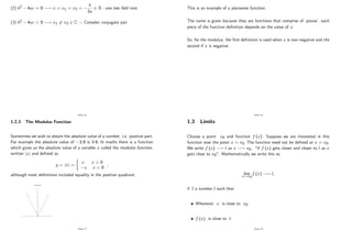
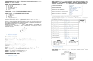
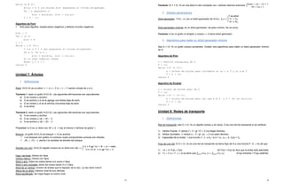
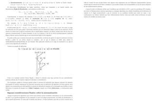
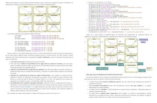
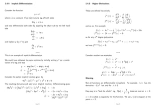
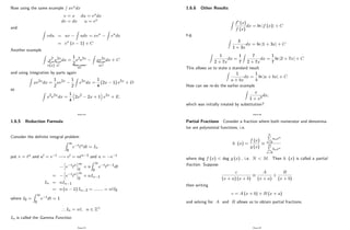
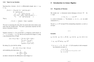
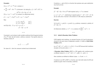
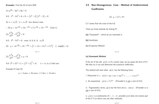
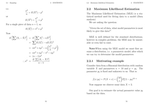
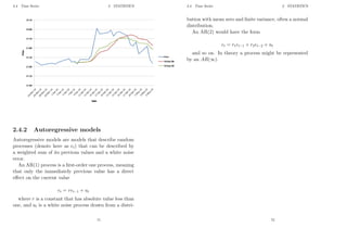
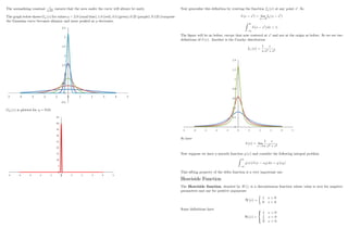
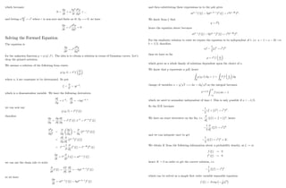
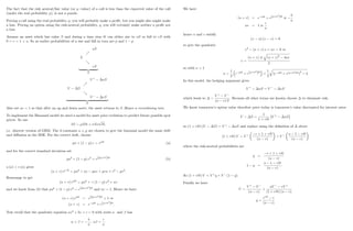
8. 1.3.2 Trigonometric/Circular Functions
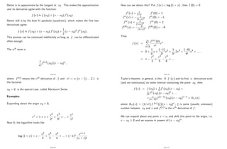
sinx and cosx
-1.5
-1
-0.5
0
0.5
1
1.5
-8 -6 -4 -2 0 2 4 6 8
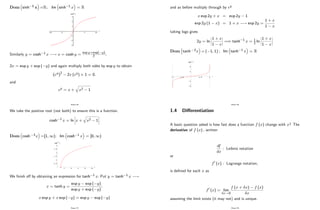
sin x is an odd function, i.e. sin ( x) = sin x:
It is periodic with period 2 : sin (x + 2 ) = sin x. This means that after
every 360 it repeats itself.
sin x = 0 () x = n 8n 2 Z
Page 28
Dom (sin x) =R and Im (sin x) = [ 1; 1]
cos x is an even function, i.e. cos ( x) = cos x:
It is periodic with period 2 : cos (x + 2 ) = cos x.
cos x = 0 () x = (2n + 1) 2 8n 2 Z
Dom (cos x) =R and Im (cos x) = [ 1; 1]
tan x =
sin x
cos x
This is an odd function: tan ( x) = tan x
Periodic: tan (x + ) = tan x
Page 29
Dom = fx : cos x 6= 0g =
n
x : x 6= (2n + 1) 2; n 2 Z
o
= R
n
(2n + 1) 2; n 2 Z
o
Trigonometric Identities:
cos2 x + sin2 x = 1; sin (x y) = sin x cos y cos x sin y
cos (x y) = cos x cos y sin x sin y; tan (x + y) =
tan x + tan y
1 tan x tan y
Exercise: Verify the following sin x + 2 = cos x; cos 2 x = sin x:
The reciprocal trigonometric functions are de…ned by
sec x =
1
cos x
; csc x =
1
sin x
; cot x =
1
tan x
Page 30
More examples on limiting:
lim
x!0
sin x ! 0; lim
x!0
sin x
x
! 1; lim
x!0
jxj ! 0
What about lim
x!0
jxj
x
?
lim
x!0+
jxj
x
= 1
lim
x!0
jxj
x
= 1
therefore
jxj
x
does not tend to a limit as x ! 0:
Page 31

9. Hyperbolic Functions
sinh x =
1
2
ex e x
Odd function: sinh ( x) = sinh x
Dom (sinh x) =R; Im (sinh x) = R
Page 32
cosh x =
1
2
ex + e x
Even function: cosh ( x) = cosh x
Dom (cosh x) =R; Im (cosh x) = [1; 1)
Page 33
tanh x =
sinh x
cosh x
Dom (tanh x) =R; Im (tanh x) = ( 1; 1)
Identities:
cosh2 x sinh2 x = 1
sinh (x + y) = sinh x cosh y + cosh x sinh y
cosh (x + y) = cosh x cosh y + sinh x sinh y
Page 34
Inverse Hyperbolic Functions
y = sinh 1 x ! x = sinh y =
exp y exp( y)
2 ;
2x = exp y exp ( y)
multiply both sides by exp y to obtain 2xey = e2y 1 which can be written
as
(ey)2
2x (ey) 1 = 0:
This gives us a quadratic in ey therefore
ey =
2x
p
4x2 + 4
2
= x
q
x2 + 1
Now
p
x2 + 1 > x =) x
p
x2 + 1 < 0 and we know that ey > 0 therefore
we have ey = x +
p
x2 + 1: Hence taking logs of both sides gives us
sinh 1 x = ln x +
q
x2 + 1
Page 35

10. Dom sinh 1 x =R; Im sinh 1 x = R
Similarly y = cosh 1 x ! x = cosh y =
exp y+exp( y)
2 ;
2x = exp y + exp ( y) and again multiply both sides by exp y to obtain
(ey)2
2x (ey) + 1 = 0:
and
ey = x +
q
x2 1
Page 36
We take the positive root (not both) to ensure this is a function.
cosh 1 x = ln x +
q
x2 1
Dom cosh 1x =[1; 1); Im cosh 1 x = [0; 1)
We …nish o¤ by obtaining an expression for tanh 1 x: Put y = tanh 1 x !
x = tanh y =
exp y exp ( y)
exp y + exp ( y)
;
x exp y + x exp ( y) = exp y exp ( y)
Page 37
and as before multiply through by ey
x exp 2y + x = exp 2y 1
exp 2y (1 x) = 1 + x ! exp 2y =
1 + x
1 x
taking logs gives
2y = ln
1 + x
1 x
=) tanh 1 x = 1
2 ln
1 + x
1 x
Dom tanh 1x = ( 1; 1) ; Im tanh 1 x = R
Page 38
1.4 Di¤erentiation
A basic question asked is how fast does a function f (x) change with x? The
derivative of f (x) ; written
df
dx
: Leibniz notation
or
f0 (x) : Lagrange notation,
is de…ned for each x as
f0 (x) = lim
x!0
f (x + x) f (x)
x
assuming the limit exists (it may not) and is unique.
Page 39

11. The term on the right hand side
f(x+ x) f(x)
x is called Newton quotient.
Di¤erentiability implies continuity but converse does not always hold.
There is another notation for a derivative due to Newton, if a function varies
with time, i.e. y = y (t) then a dot is used
y
We can also de…ne operator notation due to Euler. Write
D
d
dx
:
Then D operates on a function to produce its derivative, i.e. Df df
dx:
Page 40
The earlier form of the derivative given is also called a forward derivative.
Other possible de…nitions of the derivative are
f0 (x) = lim
x!0
1
x
(f (x) f (x x)) backward
f0 (x) = lim
x!0
1
2 x
(f (x + x) f (x x)) centred
Example: Di¤erentiating x3 from …rst principles:
f (x) = x3
f (x + x) = (x + x)3
= x3 + x3 + 3x x (x + x)
f (x + x) f (x)
x
=
x3 + 3x x (x + x)
x
= x2 + 3x2 + 3x x
! 3x2 as x ! 0;
Page 41
d
dx
xn = nxn 1;
d
dx
ex = ex;
d
dx
eax = aeax;
d
dx
log x =
1
x
;
d
dx
cos x = sin x;
d
dx
sin x = cos x;
d
dx
tan x = sec2 x
and so on. Take these as de…ned (standard results).
Examples:
f (x) = x5 ! f0 (x) = 5x4
g (x) = e3x ! g0 (x) = 3e3x = 3g (x)
Page 42
Linearity: If and are constants and y = f (x) + g (x) then
dy
dx
=
d
dx
( f (x) + g (x)) = f0 (x) + g0 (x) :
Thus if y = 3x2 6e 2x then
dy=dx = 6x + 12e 2x:
Page 43

12. 1.4.1 Product Rule
If y = f (x) g (x) then
dy
dx
= f0 (x) g (x) + f (x) g0 (x) :
Thus if y = x3e3x then
dy=dx = 3x2e3x + x3 3e3x = 3x2 (1 + x) e3x:
Page 44
1.4.2 Function of a Function Rule
Di¤erentiation is often a matter of breaking a complicated problem up into
simpler components. The function of a function rule is one of the main ways
of doing this.
If y = f (g (x)) then
dy
dx
= f0 (g (x)) g0 (x) :
Thus if y = e4x2
then
dy=dx = e4x2
4:2x = 8xe4x2
:
Page 45
So di¤erentiate the whole function, then multiply by the derivative of the
"inside" (g (x)) :
Another way to think of this is in terms of the chain rule.
Write y = f (g (x)) as
y = f (u) ; u = g (x) :
Then
dy
dx
=
d
dx
f (u) =
du
dx
d
du
f (u) = g0 (x) f0 (u)
= g0 (x) f0 (g (x)) :
Symbolically, we write this as
Page 46
dy
dx
=
du
dx
dy
du
provided u is a function of x alone.
Thus for y = e4x2
; write u = 4x2; y = eu: Then
dy
dx
=
du
dx
dy
du
= 8xe4x2
:
Further examples:
y = sin x3
y = sin u; where u = x3
y0 = cos u:3x2 ! y0 = 3x2 cos x3
y = tan2 x : this is how we write (tan x)2
so put
y = u2 where u = tan x
y0 = 2u: sec2 x ! y0 = 2 tan x sec2 x
Page 47

13. y = ln sin x: Put u = sin x ! y = ln u
dy
du
=
1
u
;
du
dx
= cos x
hence y0 = cot x:
Exercise: Di¤erentiate y = log tan2 x to show
dy
dx
= 2 sec x csc x
Page 48
1.4.3 Quotient Rule
If y =
f (x)
g (x)
then
dy
dx
=
g (x) f0 (x) f (x) g0 (x)
(g (x))2
:
Thus if y = e3x=x2;
dy
dx
=
x23e3x 2xe3x
x4
=
3x 2
x3
e3x:
This is a combination of the product rule and the function of a function (or
chain) rule. It is very simple to derive:
Page 49
Starting with y =
f (x)
g (x)
and writing as y = f (x) (g (x)) 1
we apply the
product rule
dy
dx
=
df
dx
(g (x)) 1
+ f (x)
d
dx
(g (x)) 1
Now use the chain rule on (g (x)) 1
; i.e. write u = g (x) so
d
dx
(g (x)) 1
=
du
dx
d
du
u 1 = g0 (x) u 2
=
g0 (x)
g (x)2
:
Then
dy
dx
=
1
g (x)
df
dx
f (x)
g0 (x)
g (x)2
=
f0 (x)
g (x)
f (x) g0 (x)
g (x)2
:
Page 50
To simplify we note that the common denominator is g (x)2
hence
dy
dx
=
g (x) f0 (x) f (x) g0 (x)
g (x)2
:
Examples:
d
dx
(xex) = x
d
dx
(ex) + ex d
dx
(x)
= xex + ex = ex (x + 1) ;
d
dx
(ex=x) =
x (ex)0
ex (x)0
(x)2
=
xex ex
x2
=
ex
x2
(x 1) ;
d
dx
e x2
=
d
dx
(eu) where u = x2 ) du = 2xdx
= ( 2x) e x2
:
Page 51

14. 1.4.4 Implicit Di¤erentiation
Consider the function
y = ax
where a is a constant. If we take natural log of both sides
ln y = x ln a
and now di¤erentiate both sides by applying the chain rule to the left hand
side
1
y
dy
dx
= ln a
dy
dx
= y ln a
and replace y by ax to give
dy
dx
= ax ln a:
Page 52
This is an example of implicit di¤erentiation.
We could have obtained the same solution by initially writing ax as a combi-
nation of a log and exp
y = exp (ln ax) = exp (x ln a)
y0 =
d
dx
ex ln a = ex ln a d
dx
(x ln a)
= ax ln a:
Consider the earlier implicit function given by
4y4 2y2x2 yx2 + x2 + 3 = 0:
The resulting derivative will also be an implicit function. Di¤erentiating gives
16y3y0 2 2yy0x2 + 2y2x y0x2 + 2xy = 2x
16y3 2yx2 x2 y0 = 2x + 4y2x + 2xy
y0 =
2x + 4y2x + 2xy
16y3 2yx2 x2
Page 53
1.4.5 Higher Derivatives
These are de…ned recursively;
f00 (x) =
d2f
dx2
=
d
dx
df
dx
f000 (x) =
d 3f
dx3
=
d
dx
d2f
dx2
!
and so on. For example:
f (x) = 4x3 ! f
0
(x) = 12x2 ! f00 (x) = 24x
f000 (x) = 24 ! f(iv) (x) = 0:
so for any nth degree polynomial
f (x) = anxn + an 1xn 1 + ::::::: + a1x + a0
we have f(n+1) (x) = 0:
Page 54
Consider another two examples
f (x) = ex
f0 (x) = ex ! f 00 (x) = ex
.
.
.
f(n) (x) = ex = f (x) :
g (x) = log x ! g0 (x) = 1=x
g00 (x) = 1=x2 ! g000 (x) = 2=x3:
Warning
Not all functions are di¤erentiable everywhere. For example, 1=x has the
derivative 1=x2 but only for x 6= 0:
Easy way is to "look for a hole", e.g. f (x) =
1
x 2
does not exist at x = 2:
x = 2 is called a singularity for this function. We say f (x) is singular at the
point x = 2:
Page 55

15. 1.4.6 Leibniz Rule
This is the …rst of two rules due to Leibniz. Here it is used to obtain the nth
derivative of a product y = uv, by starting with the product rule.
dy
dx
= u
dv
dx
+ v
du
dx
uDv + vDu
then
y00 = uD2v + 2DuDv + vD2u
y000 = uD3v + 3DuD2v + 3D2uDv + vD3u
and so on. This suggests (can be proved by induction)
Dn (uv) = uDnv+ n
1 DuDn 1v+ n
2 D2uDn 2v+:::+ n
r DruDn rv+:::+vDnu
where n
r = n!
r!(n r)!
:
Page 56
Example: Find the nth derivative of y = x3eax:
Put u = x3 and v = eax and Dn (uv) (uv)n ; so
(uv)n = uvn + n
1 u1vn 1 + n
2 u2vn 2 + n
3 u3vn 3 + :::::::
u = x3; u1 = 3x2; u2 = 6x; u3 = 6; u4 = 0
v = eax; v1 = aeax; v2 = a2eax; ::::::::; vn = aneax
therefore Dn x3eax =
x3aneax + n
1 3x2an 1eax + n
2 6xan 2eax + n
3 6an 3eax
= eax x3an + n3x2an 1 + n (n 1) an 23x + n (n 1) (n 2) an 3
Page 57
1.4.7 Further Limits
This will be an application of di¤erentiation. Consider the limiting case
lim
x!a
f (x)
g (x)
0
0
or
1
1
This is called an indeterminate form. Then L’Hospitals rule states
lim
x!a
f (x)
g (x)
= lim
x!a
f 0 (x)
g0 (x)
= ::::::: = lim
x!a
f(r) (x)
g(r) (x)
for r such that we have the indeterminate form 0=0: If for r + 1 we have
lim
x!a
f(r+1) (x)
g(r+1) (x)
! A
where A is not of the form 0=0 then
lim
x!a
f (x)
g (x)
lim
x!a
f(r+1) (x)
g(r+1) (x)
:
Page 58
Note: Very important to verify quotient has this indeterminate form before
using L’
Hospitals rule. Else we end up with an incorrect solution.
Examples:
1.
lim
x!0
cos x + 2x 1
3x
0
0
So di¤erentiate both numerator and denominator !
lim
x!0
d
dx (cos x + 2x 1)
d
dx (3x)
= lim
x!0
sin x + 2
3
6=
0
0
!
2
3
2. lim
x!0
ex + e x 2
1 cos 2x
; quotient has form 0=0: By L’Hospital’
s rule we have
lim
x!0
ex e x
2 sin 2x
; which has indeterminate form 0=0 again for 2nd time, so
Page 59

16. we apply L’Hospital’
s rule again
lim
x!0
ex + e x
4 cos 2x
=
1
2
:
3. lim
x!1
x2
ln x
1
1
) use L’
Hospital , so lim
x!1
2x
1=x
! 1
4. lim
x!1
e3x
ln x
1
1
) lim
x!1
3xe3x ! 1
5. lim
x!1
x2e 3x 0:1; so we convert to form 1=1 by writing lim
x!1
x2
e3x
;
and now use L’
Hospital (di¤erentiate twice), which gives lim
x!1
2
9e3x
! 0
Page 60
6. lim
x!0
sin x
x
lim
x!0
cos x 1
What is example 6: saying?
When x is very close to 0 then sin x x: That is sin x can be approximated
with the function x for small values.
Page 61
1.5 Taylor Series
Many functions are so complicated that it is not easy to see what they look
like. If we only want to know what a function looks like locally , we can
approximate it by simpler functions: polynomials. The crudest approximation
is by a constant: if f (x) is continuous at x0;
f (x) t f (x0)
for x near x0:
Before we consider this in a more formal manner we start by looking at a simple
motivating example:
Consider f (x) = ex:
Page 62
Suppose we wish to approximate this function for very small values of x (i.e.
x ! 0). We know at x = 0; df
dx = 1: So this is the gradient at x = 0: We
can …nd the equation of the line that passes through a point (x0; y0) using
y y0 = m (x x0) :
Here m = df
dx = 1; x0 = 0; y0 = 1; so y = 1 + x; is a polynomial. What
information have we ascertained from this?
If x ! 0 then the point (x; 1 + x) on the tangent is close to the point
(x; ex) on the graph f (x) and hence
Page 63

17. ex 1 + x
-5
0
5
10
15
20
25
-4 -3 -2 -1 0 1 2 3 4
Page 64
Suppose now that we are not that close to 0: We look for a second degree
polynomial (i.e. quadratic)
g (x) = ax2 + bx + c ! g0 = 2ax + b ! g00 = 2a
If we want this parabola g (x) to have
(i) same y intercept as f :
g (0) = f (0) =) c = 1
(ii) same tangent as f
g0 (0) = f0 (0) =) b = 1
(iii) same curvature as f
g00 (0) = f00 (0) =) 2a = 1
Page 65
This gives
ex g (x) =
1
2
x2 + x + 1
0
5
10
15
20
25
-4 -3 -2 -1 0 1 2 3 4
Page 66
Moving further away we would look at a third order polynomial h (x) which
gives
ex h (x) =
1
3!
x3 +
1
2!
x2 + x + 1
-5
0
5
10
15
20
25
-4 -3 -2 -1 0 1 2 3 4
and so on.
Page 67

18. Better is to approximate by the tangent at x0: This makes the approximation
and its derivative agree with the function:
f (x) t f (x0) + (x x0) f0 (x0) :
Better still is by the best …t parabola (quadratic), which makes the …rst two
derivatives agree:
f (x) t f (x0) + (x x0) f0 (x0) +
1
2
(x x0)2
f00 (x0) :
This process can be continued inde…nitely as long as f can be di¤erentiated
often enough.
The nth term is
1
n!
f(n) (x0) (x x0)n
;
Page 68
where f(n) means the nth derivative of f and n! = n: (n 1) : : : 2:1 is
the factorial.
x0 = 0 is the special case, called Maclaurin Series.
Examples:
Expanding about the origin x0 = 0;
ex = 1 + x +
x2
2!
+
x3
3!
+ ::: +
xn
n!
Near 0; the logarithm looks like
log (1 + x) = x
x2
2
+
x3
3
x4
4
+ ::: + ( 1)n xn+1
(n + 1)!
Page 69
How can we obtain this? Put f (x) = log (1 + x) ; then f (0) = 0
f0 (x) = 1
1+x f0 (0) = 1
f00 (x) = 1
(1+x)2 f00 (0) = 1
f000 (x) = 2
(1+x)3 f000 (0) = 2
f(4) (x) = 6
(1+x)4 f(4) (0) = 6
Thus
f (x) =
1
X
n=0
f(n) (0)
n!
xn
= 0 +
1
1!
x +
( 1)
2!
x2 +
1
3!
:2x3 +
( 6)
4!
x4 + :::::
= x
x2
2
+
x3
3
x4
4
+ :::
Page 70
Taylor’
s theorem, in general, is this : If f (x) and its …rst n derivatives exist
(and are continuous) on some interval containing the point x0 then
f (x) = f (x0) + 1
1!f0 (x0) (x x0) +
1
2!f00 (x0) (x x0)2
+ :::
+ 1
(n 1)!
f(n 1) (x0) (x x0)n 1
+ Rn (x)
where Rn (x) = (1=n!) f (n) ( ) (x x0)n
; is some (usually unknown)
number between x0 and x and f(n) is the nth derivative of f.
We can expand about any point x = a; and shift this point to the origin, i.e.
x x0 0 and we express in powers of (x x0)n
:
Page 71

19. So for f (x) = sin x about x = =4 we will have
f (x) =
1
X
n=0
f(n)
4
n!
(x =4)n
where f(n)
4 is the nth derivative of sin x at x0 = =4:
As another example suppose we wish to expand log (1 + x) about x0 = 2; i.e.
x 2 = 0 then
f (x) =
1
X
n=0
1
n!
f(n) (2) (x 2)n
where f(n) (2) is the nth derivative of log (1 + x) evaluated at the point
x = 2:
Note that log (1 + x) does not exist for x = 1:
Page 72
1.5.1 The Binomial Expansion
The Binomial Theorem is the Taylor expansion of (1 + x)n
where n is a
positive integer. It reads:
(1 + x)n
= 1 + nx +
n (n 1)
2!
x2 +
n (n 1) (n 2)
3!
x3 + ::: :
We can extend this to expressions of the form
(1 + ax)n
= 1 + n (ax) +
n(n 1)
2! (ax)2
+
n(n 1)(n 2)
3! (ax)3
+ ::: :
(p + ax)n
=
"
p 1 +
a
p
x
!#n
= pn
"
1 + n
a
p
x
!
+ ::::::::
#
Page 73
The binomial coe¢ cients are found in Pascal’
s triangle:
1 (n=0) (1 + x)0
1 1 (n=1) (1 + x)1
1 2 1 (n=2) (1 + x)2
1 3 3 1 (n=3) (1 + x)3
1 4 6 4 1 (n=4) (1 + x)4
1 5 10 10 5 1 (n=5) (1 + x)5
and so on ...
Page 74
As an example consider:
(1 + x)3
n = 3 ) 1 3 3 1 ) (1 + x)3
= 1 + 3x + 3x2 + x3
(1 + x)5
n = 5 ! (1 + x)5
= 1 + 5x + 10x2 + 10x3 + 5x4 + x5:
If n is not an integer the theorem still holds but the coe¢ cients are no longer
integers. For example,
(1 + x) 1
= 1 x + x2 x3 + ::: :
and
(1 + x)1=2
= 1 +
1
2
x +
1
2
1
2
x2
2!
::: :
Page 75

20. (a + b)k
= ak
h
1 + b
a
ik
=
ak 1 + kba 1 +
k(k 1)
2! b2a 2 +
k(k 1)(k 2)
3! b3a 3 + ::
= ak + kbak 1 +
k(k 1)
2 b2ak 2 +
k(k 1)(k 2)
3! b3ak 3 + ::
Example: We looked at lim
x!0
sin x
x
! 1 (by L’
Hospital). We can also do this
using Taylor series:
lim
x!0
sin x
x
lim
x!0
x x3=3! + x5=5! + ::::
x
lim
x!0
1 x2=3! + x4=5! + ::::
! 1:
Page 76
1.6 Integration
1.6.1 The Inde…nite Integral
The inde…nite integral of f (x) ;
Z
f (x) dx;
is any function F (x) whose derivative equals f (x). Thus if
F (x) =
Z
f (x) dx then
dF
dx
(x) = f (x) :
Since the derivative of a constant, C; is zero (dC=dx = 0) ; the inde…nite
integral of f (x) is only determined up to an arbitrary constant.
Page 77
If
dF
dx
= f (x) then
d
dx
(F (x) + C) =
dF
dx
(x) +
dC
dx
=
dF
dx
(x) = f (x) :
Thus we must always include an arbitrary constant of integration in an inde…nite
integral.
Simple examples are
Z
xndx =
1
n + 1
xn+1 + C (n 6= 1) ;
Z
dx
x
= log (x) + C;
Z
eaxdx =
1
a
eax + C (a 6= 0) ;
Z
cos axdx =
1
a
sin ax + C;
Z
sin axdx =
1
a
cos ax + C
Page 78
Linearity
Integration is linear:
Z
( f (x) + g (x)) dx =
Z
f (x) dx +
Z
g (x) dx
for constants A and B: Thus, for example
Z
Ax2 + Bx3 dx = A
Z
x2dx + B
Z
x3dx
=
A
3
x3 +
B
4
x4 + C;
Z
(3ex + 2=x) dx = 3
Z
exdx + 2
Z
dx
x
= 3ex + 2 log (x) + C;
and so forth.
Page 79

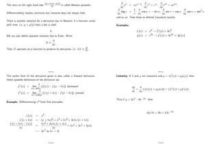
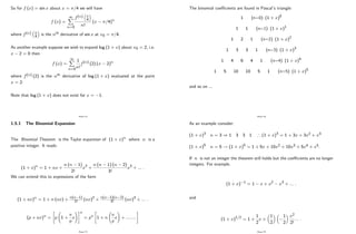
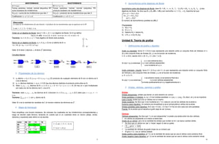
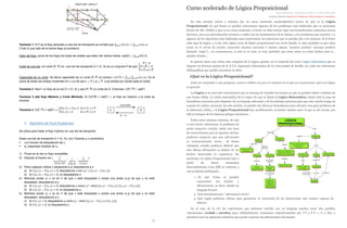
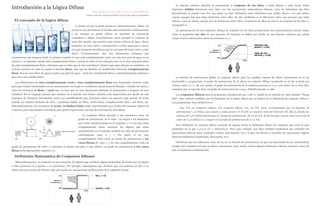
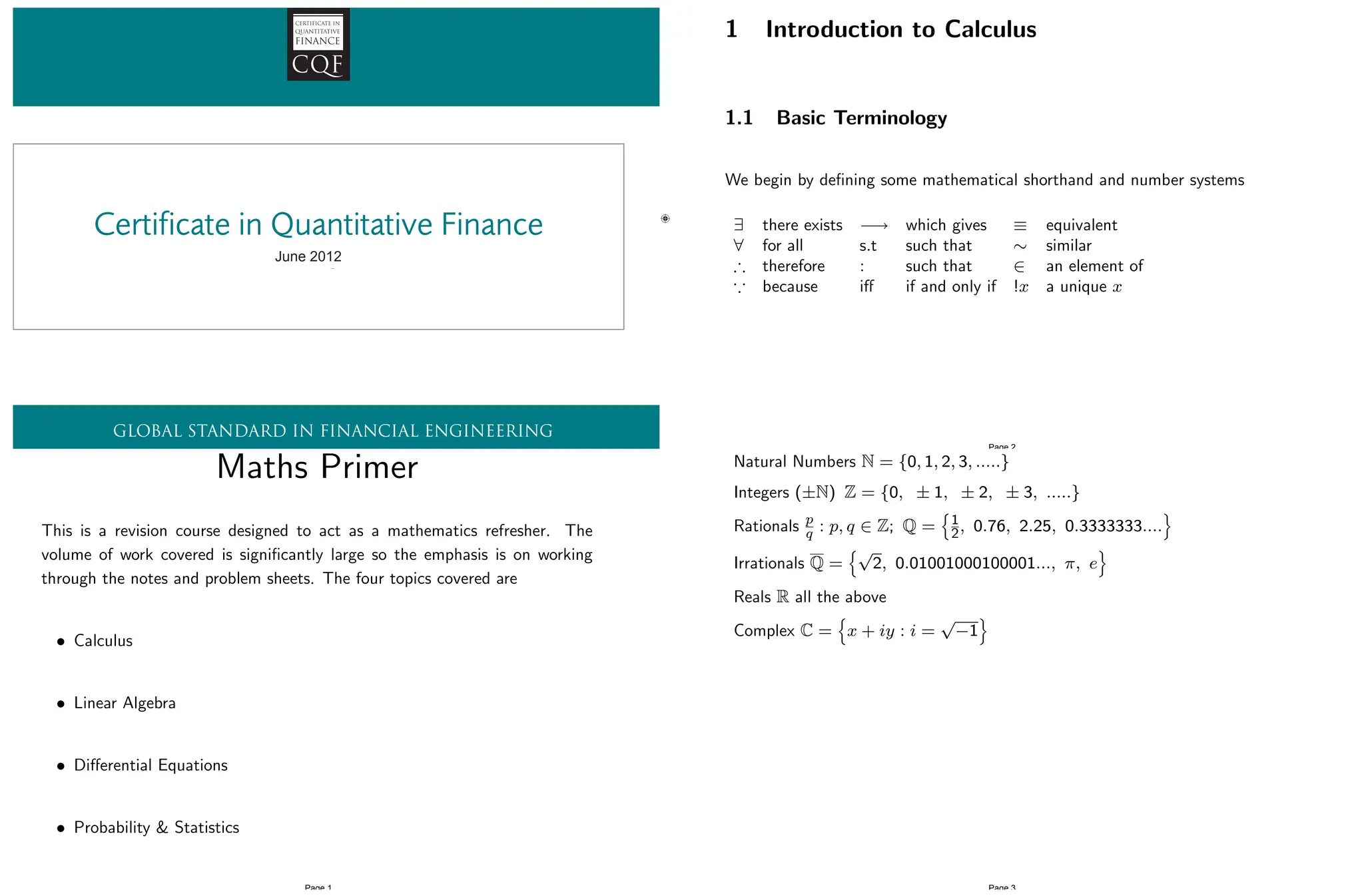
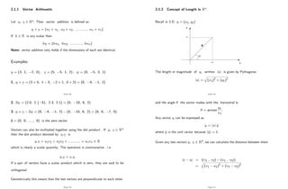
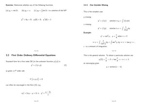
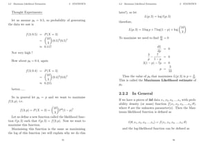
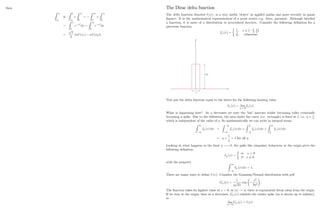
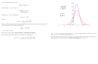
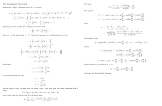
21. 1.6.2 The De…nite Integral
The de…nite integral,
Z b
a
f (x) dx;
is the area under the graph of f (x) ; between x = a and x = b; with
positive values of f (x) giving positive area and negative values of f (x)
contributing negative area. It can be computed if the inde…nite integral is
known. For example
Z 3
1
x3dx =
1
4
x4
3
1
=
1
4
34 14 = 20;
Z 1
1
exdx = [ex]1
1 = e 1=e:
Note that the de…nite integral is also linear in the sense that
Z b
a
(Af (x) + Bg (x)) dx = A
Z b
a
f (x) dx + B
Z b
a
g (x) dx:
Page 80
Note also that a de…nite integral
Z b
a
f (x) dx
does not depend on the variable of integration, x in the above, it only depends
on the function f and the limits of integration (a and b in this case); the
area under a curve does not depend on what we choose to call the horizontal
axis.
So
Z b
a
f (x) dx =
Z b
a
f (y) dy =
Z b
a
f (z) dz:
We should never confuse the variable of integration with the limits of integra-
tion; a de…nite integral of the form
Z x
a
f (x) dx;
use dummy variable.
Page 81
If a < b < c then
Z c
a
f (x) dx =
Z b
a
f (x) dx +
Z c
b
f (x) dx:
Also
Z a
c
f (x) dx =
Z c
a
f (x) dx:
Page 82
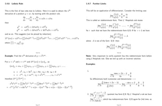
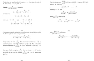
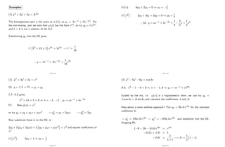
1.6.3 Integration by Substitution
This involves the change of variable and used to evaluate integrals of the form
Z
g (f (x)) f0 (x) dx;
and can be evaluated by writing z = f (x) so that dz=dx = f0 (x) or
dz = f0 (x) dx: Then the integral becomes
Z
g (z) dz:
Examples:
Z
x
1 + x2
dx : z = 1 + x2 ! dz = 2xdx
Z
x
1 + x2
dx =
1
2
log (z) + C =
1
2
log 1 + x2 + C
= log
q
1 + x2 + C
Page 83

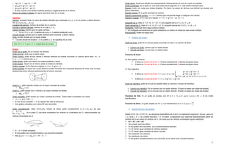
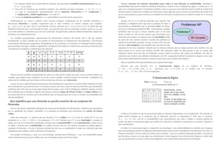
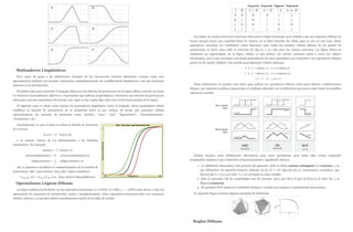
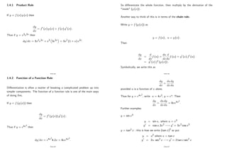
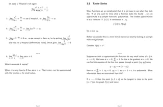
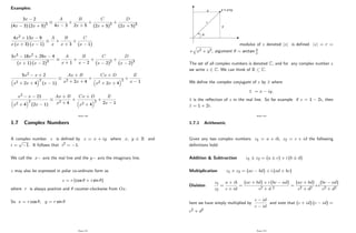
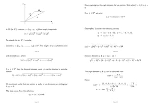
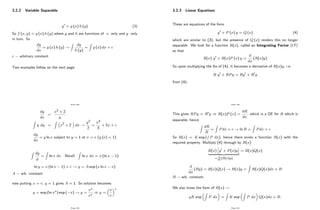
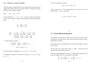
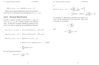
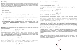
22. R
xe x2
dx : z = x2 ! dz = 2xdx
Z
xe x2
dx =
1
2
Z
ezdz
=
1
2
ez + C =
1
2
e x2
+ C
Z
1
x
log (x) dx =
Z
z dz =
1
2
z2 + C
=
1
2
(log (x))2
+ C
with z = log (x) so dz = dx=x and
Z
ex+ex
dx =
Z
exeex
dx =
Z
ezdz
= ez + C = eex
+ C
with z = ex so dz = exdx:
Page 84
The method can be used for de…nite integrals too. In this case it is usually more
convenient to change the limits of integration at the same time as changing
the variable; this is not strictly necessary, but it can save a lot of time.
For example, consider
Z 2
1
ex2
2xdx:
Write z = x2; so dz = 2xdx: Now consider the limits of integration; when
x = 2; z = x2 = 4 and when x = 1; z = x2 = 1: Thus
Z x=2
x=1
ex2
2xdx =
Z z=4
z=1
ezdz
= [ez]z=4
z=1 = e4 e1:
Page 85
Further examples: consider
Z x=2
x=1
2xdx
1 + x2
:
In this case we could write z = 1 + x2; so dz = 2xdx and x = 1
corresponds to z = 2, x = 2 corresponds to z = 5; and
Z x=2
x=1
2x
1 + x2
dx =
Z z=5
z=2
dz
z
= [ln (z)]z=5
z=2 = log (5) ln (2)
= ln (5=2)
We can solve the same problem without change of limit, i.e.
n
ln 1 + x2
ox=2
x=1
! ln 5 ln 2 = ln 5=2:
Page 86
Or consider
Z x=e
x=1
2
log (x)
x
dx
in which case we should choose z = log (x) so dz = dx=x and x = 1
gives z = 0; x = e gives z = 1 and so
Z x=e
x=1
2
log (x)
x
dx =
Z z=1
z=0
2zdz =
h
z2
iz=1
z=0
= 1:
Page 87

23. When we make a substitution like z = f (x) we are implicitly assuming that
dz=dx = f 0 (x) is neither in…nite nor zero. It is important to remember this
implicit assumption.
Consider the integral
Z 1
1
x2dx =
1
3
h
x3
ix=1
x= 1
=
1
3
(1 ( 1)) =
2
3
:
Now put z = x2 so dz = 2xdx or dz = 2
p
z dx and when x = 1;
z = x2 = 1 and when x = 1; z = x2 = 1; so
Z x=1
x= 1
x2dx =
1
2
Z z=1
z=1
dz
p
z
= 0
as the area under the curve 1=
p
z between z = 1 and z = 1 is obviously
zero.
Page 88
It is clear that x2 > 0 except at x = 0 and therefore that
Z 1
1
x2dx =
2
3
must be the correct answer. The substitution z = x2 gave
Z x=1
x= 1
x2dx =
1
2
Z z=1
z=1
dz
p
z
= 0
which is obviously wrong. So why did the substitution fail?
It failed because f 0 (x) = dz=dx = 2x changed signs between x = 1
and x = 1: In particular, dz=dx = 0 at x = 0; the function z = x2 is
not invertible for 1 x 1:
Moral: when making a substitution make sure that dz=dx 6= 0:
Page 89
1.6.4 Integration by Parts
This is based on the product rule. In usual notation, if y = u (x) v (x) then
dy
dx
=
du
dx
v + u
dv
dx
so that
du
dx
v =
dy
dx
u
dv
dx
and hence integrating
Z
du
dx
vdx =
Z
dy
dx
dx
Z
u
dv
dx
dx = y (x)
Z
u
dv
dx
dx + C
or
Z
du
dx
vdx = u (x) v (x)
Z
u (x)
dv
dx
dx + C
i.e.
Z
u0vdx = uv
Z
uv0dx + C
Page 90
This is useful, for instance, if v (x) is a polynomial and u (x) is an exponential.
How can we use this formula? Consider the example
Z
xexdx
Put
v = x u0 = ex
v0 = 1 u = ex
hence
Z
xexdx = uv
Z
u
dv
dx
dx
= xex
Z
ex:1dx = ex (x 1) + C
The formula we are using is the same as
Z
vdu = uv
Z
udv + C
Page 91

24. Now using the same example
R
xexdx
v = x du = exdx
dv = dx u = ex
and
Z
vdu = uv
Z
udv = xex
Z
exdx
= ex (x 1) + C
Another example
Z
x2
|{z}
v(x)
e2x
|{z}
u0
dx =
1
2
x2e2x
| {z }
uv
Z
xe2x
| {z }
uv0
dx + C
and using integration by parts again
Z
xe2xdx =
1
2
xe2x 1
2
Z
e2xdx =
1
4
(2x 1) e2x + D
so Z
x2e2xdx =
1
4
2x2 2x + 1 e2x + E:
Page 92
1.6.5 Reduction Formula
Consider the de…nite integral problem
Z 1
0
e ttndt = In
put v = tn and u0 = e t ! v0 = ntn 1 and u = e t
h
e ttn
i1
0
+ n
Z 1
0
e ttn 1dt
=
h
e ttn
i1
0
+ nIn 1
In = nIn 1
= n (n 1) In 2 = ::::::: = n!I0
where I0 =
Z 1
0
e tdt = 1
) In = n!; n 2 Z+
In is called the Gamma Function.
Page 93
1.6.6 Other Results
Z
f0 (x)
f (x)
dx = ln jf (x)j + C
e.g.
Z
3
1 + 3x
dx = ln j1 + 3xj + C
Z
1
2 + 7x
dx =
1
7
Z
7
2 + 7x
dx =
1
7
ln j2 + 7xj + C
This allows us to state a standard result
Z
1
a + bx
dx =
1
b
ln ja + bxj + C
How can we re-do the earlier example
Z
x
1 + x2
dx;
which was initially treated by substitution?
Page 94
Partial Fractions Consider a fraction where both numerator and denomina-
tor are polynomial functions, i.e.
h (x) =
f (x)
g (x)
N
P
n=0
anxn
M
P
n=0
bnxn
where deg f (x) < deg g (x) , i.e. N < M: Then h (x) is called a partial
fraction. Suppose
c
(x + a) (x + b)
A
(x + a)
+
B
(x + b)
then writing
c = A (x + b) + B (x + a)
and solving for A and B allows us to obtain partial fractions.
Page 95

25. The simplest way to achieve this is by setting x = b to obtain the value of
B; then putting x = a yields A:
Example:
1
(x 2) (x + 3)
: Now write
1
(x 2) (x + 3)
A
x 2
+
B
x + 3
which becomes
1 = A (x + 3) + B (x 2)
Setting x = 3 ! B = 1=5; x = 2 ! A = 1=5: So
1
(x 2) (x + 3)
1
5 (x 2)
1
5 (x + 3)
:
Page 96
There is another quicker and simpler method to obtain partial fractions, called
the "cover-up" rule. As an example consider
x
(x 2) (x + 3)
A
x 2
+
B
x + 3
:
Firstly, look at the term
A
x 2
: The denominator vanishes for x = 2; so
take the expression on the LHS and "cover-up" (x 2) : Now evaluate the
remaining expression, i.e.
x
(x + 3)
for x = 2; which gives 2=5: So A = 2=5:
Now repeat this, by noting that
B
x + 3
does not exist at x = 3: So cover
up (x + 3) on the LHS and evaluate
x
(x 2)
for x = 3; which gives
B = 3=5:
Page 97
Any rational expression
f (x)
g (x)
(with degree of f(x) < degree of g(x)) such
as above can be written
f (x)
g (x)
F1 + F2 + :::::::: + Fk
where each Fi has form
A
(px + q)m or
Cx + D
ax2 + bx + c
n
where
A
(px + q)m is written as
A1
(px + q)
+
A2
(px + q)2
+ :::::: +
A
(px + q)m
Page 98
and
Cx + D
ax2 + bx + c
n becomes
C1x + D1
ax2 + bx + c
+ :::::: +
Cnx + Dn
ax2 + bx + c
n
Page 99

26. Examples:
3x 2
(4x 3) (2x + 5)3
A
4x 3
+
B
2x + 5
+
C
(2x + 5)2
+
D
(2x + 5)3
4x2 + 13x 9
x (x + 3) (x 1)
A
x
+
B
x + 3
+
C
(x 1)
3x3 18x2 + 29x 4
(x + 1) (x 2)3
A
x + 1
+
B
x 2
+
C
(x 2)2
+
D
(x 2)3
5x2 x + 2
x2 + 2x + 4
2
(x 1)
Ax + B
x2 + 2x + 4
+
Cx + D
x2 + 2x + 4
2
+
E
x 1
x2 x 21
x2 + 4
2
(2x 1)
Ax + B
x2 + 4
+
Cx + D
x2 + 4
2
+
E
2x 1
Page 100
1.7 Complex Numbers
A complex number z is de…ned by z = x + iy where x; y 2 R and
i =
p
1: It follows that i2 = 1:
We call the x axis the real line and the y axis the imaginary line.
z may also be expressed in polar co-ordinate form as
z = r (cos + i sin )
where r is always positive and counter-clockwise from Ox:
So x = r cos ; y = r sin
Page 101
x
y
r
θ
z = x+iy
modulus of z denoted jzj is de…ned jzj = r =
+
q
x2 + y2; argument = arctan y
x
The set of all complex numbers is denoted C; and for any complex number z
we write z 2 C: We can think of R C:
We de…ne the complex conjugate of z by
_
z where
_
z = x iy:
z is the re‡ection of z in the real line. So for example if z = 1 2i; then
z = 1 + 2i:
Page 102
1.7.1 Arithmetic
Given any two complex numbers z1 = a + ib; z2 = c + id the following
de…nitions hold:
Addition & Subtraction z1 z2 = (a c) + i (b d)
Multiplication z1 z2 = (ac bd) + i (ad + bc)
Division
z1
z2
=
a + ib
c + id
=
(ac + bd) + i (bc ad)
c2 + d 2
=
(ac + bd)
c2 + d2
+i
(bc ad)
c2 + d2
here we have simply multiplied by
c id
c id
and note that (c + id) (c id) =
c2 + d2
Page 103

27. Examples
z1 = 1 + 2i; z2 = 3 i
z1 +z2 = (1 + 3)+i (2 1) = 4+i ; z1 z2 = (1 3) i (2 ( 1)) =
2 + 3i
z1 z2 = (1:3 2: 1) + i (1: 1 + 2:3) = 5 + 5i
z1
z2
=
1 + 2i
3 i
:
3 + i
3 + i
=
1
10
+ i
7
10
Page 104
1.7.2 Complex Conjugate Identities
1.
_
z = z
2. (z1 + z2) = z1 +
_
z2
3. (z1z2) =
_
z1
_
z2
4. z +
_
z = 2x = 2 Re z ) Re z =
z +
_
z
2
5. z
_
z = 2iy = 2i Im z ) Im z =
z
_
z
2i
6. z:
_
z = (x + iy) (x iy) = jzj2
Page 105
7. jzj2
= z(z) = zz = jzj2
) jzj = jzj
8.
z1
z2
=
z1
z2
:
z2
z2
=
z1z2
jz2j2
9. jz1z2j2
= jz1j2
jz2j2
Page 106
1.7.3 Polar Form
We return to the polar form representation of complex numbers. We now
introduce a new notation. If z 2 C; then
z = r (cos + i sin ) = rei :
Hence
ei = cos + i sin ;
which is a special relationship called Euler’
s Identity. Knowing sin is an odd
function gives e i = cos i sin : Referring to the earlier polar coordinate
…gure, we have:
jzj = r; arg z =
If
z1 = r1ei 1 and z2 = r2ei 2
Page 107

28. then
z1z2 = r1r2ei( 1+ 2) ) jz1z2j = r1r2 = jz1j jz2j
arg (z1z2) = 1 + 2 = arg (z1) + arg (z2) :
If z2 6= 0 then
z1
z2
=
r1ei 1
r2ei 2
=
r1
r2
ei( 1 2)
and hence
z1
z2
=
jz1j
jz2j
=
r1
r2
arg
z1
z2
!
= 1 2 = arg (z1) arg (z2)
Page 108
Euler’
s Formula Let be any a1ngle, then
exp (i ) = cos + i sin :
We can prove this by considering the Taylor series for exp (x) ; sin x; cos x
ex = 1 + x +
x2
2!
+
x3
3!
+ ::::::::::::: +
xn
n!
(a)
sin x = x
x3
3!
+
x5
5!
::::::::::::: + ( 1)n x2n+1
(2n + 1)!
(b)
cos x = 1
x2
2!
+
x4
4!
::::::::::::: + ( 1)n x2n
(2n)!
(c)
Page 109
Replacing x by the purely imaginary quantity i in (a), we obtain
ei = 1 + i +
(i )2
2!
+
(i )3
3!
+ ::::::::::::: +
(i )n
n!
= 1
2
2!
+
4
4!
6
6!
+ ::::::::::::
!
+
i
3
3!
+
5
5!
:::::::::
!
= cos + i sin
Note: When = then exp i = 1 and = =2 gives exp (i =2) = i:
Page 110
We can apply Euler’
s formula to integral problems. Consider the problem
Z
ex sin xdx
which was simpli…ed using the integration by parts method. We know Re ei =
cos ; so the above becomes
Z
ex Im eixdx =
Z
Im e(i+1)xdx = Im 1
1+ie(i+1)x
= ex Im 1
1+i eix = ex Im 1 i
(1+i)(1 i)
eix
= 1
2ex Im (1 i) eix = 1
2ex Im eix ieix
= 1
2ex Im (cos x + i sin x i cos x + sin x)
= 1
2ex (sin x cos x)
Exercise: Apply this method to solving
Z
ex cos xdx.
Page 111

29. 1.8 Functions of Several Variables: Multivariate Calculus
A function can depend on more than one variable. For example, the value of
an option depends on the underlying asset price S (for ’
spot’or ’
share’
) and
time t: We can write its value as V (S; t) :
The value also depends on other parameters such as the exercise price E;
interest rate r and so on. Although we could write V (S; t; E; r; :::) ; it is
usually clearer to leave these other variables out.
Depending on the application, the independent variables may be x and t for
space and time, or two space variables x and y; or S and t for price and
time, and so on.
Page 112
Consider a function z = f (x; y) ; which can be thought of as a surface in
x; y; z space. We can think of x and y as positions on a two dimensional
grid (or as spacial variables) and z as the height of a surface above the (x; y)
grid.
How do we di¤erentiate a function f (x; y) of two variables? What if there
are more independent variables?
The partial derivative of f (x; y) with respect to x is written
@f
@x
(note @ and not d ). It is the x derivative of f with y held …xed:
@f
@x
= lim
x!0
f (x + x; y) f (x; y)
x
:
Page 113
The other partial derivative, @f=@y; is de…ned similarly but now x is held
…xed:
@f
@y
= lim
y!0
f (x; y + y) f (x; y)
y
:
@f
@x
and
@f
@y
are sometimes written as fx and fy:
Examples
If
f (x; y) = x + y2 + xe y2
then
@f
@x
= fx = 1 + 0 + 1 e y2
Page 114
@f
@y
= fy = 0 + 2y + x ( 2y) e y2
:
The convention is, treat the other variable like a constant.
Page 115

30. Higher Derivatives
Like ordinary derivatives, these are de…ned recursively:
@2f
@x2
= fxx =
@
@x
@f
@x
;
@2f
@y2
= fyy =
@
@y
@f
@y
!
:
and
@2f
@x@y
= fxy =
@
@y
@f
@x
;
@2f
@y@x
= fyx =
@
@x
@f
@y
!
:
Page 116
If f is well-behaved, the ’
mixed’partial derivatives are equal:
fxy = fyx:
i.e. the second order derivatives exist and are continuous.
Example:
With f (x; y) = x + y2 + xe y2
as above,
fx = 1 + e y2
so
fxx = 0; fxy = 2ye y2
Page 117
Also
fy = 2y 2xye y2
so
fyx = 2ye y2
; fyy = 2 2xe y2
+ 4xy2e y2
Note that fxy = fyx:
Page 118
1.8.1 The Chain Rule I
Suppose that x = x (s) and y = y (s) and F (s) = f (x (s) ; y (s)) :
Then
dF
ds
(s) =
@f
@x
(x (s) ; y (s))
dx
ds
(s) +
@f
@y
(x (s) ; y (s))
dy
ds
(s)
Thus if f (x:y) = x2 + y2 and x (s) = cos (s) ; y (s) = sin (s) we …nd
that F (s) = f (x (s) ; y (s)) has derivative
dF
ds
= sin (s) 2 cos (s) + cos (s) 2 sin (s) = 0
which is what it should be, since F (s) = cos2 (s) + sin2 (s) = 1;
i.e. a constant.
Page 119

31. Example: Calculate
dz
dt
at t = =2 where
z = exp xy2 x = t cos t; y = t sin t:
Chain rule gives
dz
dt
=
@z
@x
dx
dt
+
@z
@y
dy
dt
= y2 exp xy2 ( t sin t + cos t) +
2xy exp xy2 (sin t + t cos t) :
At t = =2 x = 0; y = =2 )
dz
dt t= =2
=
3
8
:
Page 120
1.8.2 The Chain Rule II
Suppose that x = x (u; v) ; y = y (u; v) and that F (u; v) = f (x (u; v) ; y (u; v)) :
Then
@F
@u
=
@x
@u
@f
@x
+
@y
@u
@f
@y
and
@F
@v
=
@x
@v
@f
@x
+
@y
@v
@f
@y
:
This is sometimes written as
@
@u
=
@x
@u
@
@x
+
@y
@u
@
@y
;
@
@v
=
@x
@v
@
@x
+
@y
@v
@
@y
:
so is essentially a di¤erential operator.
Page 121
Example:
T = x3 xy + y3 where x = r cos ; y = r sin
@T
@r
=
@T
@x
@x
@r
+
@T
@y
@y
@r
= cos 3x2 y + sin 3y2 x
= cos 3r2 cos2 r sin +
sin 3r2 sin2 r cos
= 3r2 cos3 + sin3 2r cos sin
= 3r2 cos3 + sin3 r sin 2 :
Page 122
@T
@
=
@T
@x
@x
@
+
@T
@y
@y
@
= r sin 3x2 y + r cos 3y2 x
= r sin 3r2 cos2 r sin +
r cos 3r2 sin2 r cos
= 3r3 cos sin (sin cos ) +
r2 sin2 cos2 :
= r2 (sin cos ) (3r cos sin + sin + cos )
Page 123

32. 1.8.3 Taylor for two Variables
Assuming that a function f (x; t) is di¤erentiable enough, near x = x0;
t = t0;
f (x; t) = f (x0; t0) + (x x0) fx (x0; t0) +
(t t0) ft (x0; t0)
+
1
2
2
6
4
(x x0)2
fxx (x0; t0)
+2 (x x0) (t t0) fxt (x0; t0)
+ (t t0)2
ftt (x0; t0)
3
7
5 + ::::
That is,
f (x; t) = constant + linear + quadratic
+::::
The error in truncating this series after the second order terms tends to zero
faster than the included terms. This result is particularly important for Itô’
s
lemma in Stochastic Calculus.
Page 124
Suppose a function f = f (x; y) and both x; y change by a small amount, so
x ! x + x and y ! y + y; then we can examine the change in f using
a two dimensional form of Taylor
f (x + x; y + y) = f (x; y) + fx x + fy y +
1
2
fxx x2 +
1
2
fyy y2 +
fxy x y + O x2; y2 :
By taking f (x; y) to the lhs, writing
df = f (x + x; y + y) f (x; y)
and considering only linear terms, i.e.
df =
@f
@x
x +
@f
@y
y
we obtain a formula for the di¤erential or total change in f:
Page 125
2 Introduction to Linear Algebra
2.1 Properties of Vectors
We consider real n dimensional vectors belonging to the set Rn. An
n tuple
v = (v1; v2; :::::::::; vn) 2 Rn
is a vector of dimension n: The elements vi (i = 1; ::::; n) are called
components of v:
Any pair u; v 2 Rn are equal i¤ the corresponding components ui’
s and vi’
s
are equal
Page 126
Examples:
u1 = (1; 0) ; u2 = 1; e;
p
3; 6 ; u3 = (3; 4) ; u4 = ( ; ln 3; 2; 1)
1. u1 ; u3 2 R2 and u2 ; u4 2 R4
2. (x + y; x z; 2z 1) = (3; 2; 5) :For equality to hold correspond-
ing components are equal, so
x + y = 3
x z = 2
2z 1 = 5
9
>
=
>
;
) x = 1; y = 2; z = 3
Page 127

33. 2.1.1 Vector Arithmetic
Let u; v 2 Rn: Then vector addition is de…ned as
u + v = (u1 + v1; u2 + v2; :::::::::::; un + vn)
If k 2 R is any scalar then
ku = (ku1; ku2; :::::::::::; kun)
Note: vector addition only holds if the dimensions of each are identical.
Examples:
u = (3; 1; 2; 0) ; v = (5; 5; 1; 2) ; w = (0; 5; 3; 1)
1. u + v = (3 + 5; 1 5; 2 + 1; 0 + 2) = (8; 4; 1; 2)
Page 128
2. 2w = (2:0; 2: ( 5) ; 2:3; 2:1) = (0; 10; 6; 2)
3. u + v 2w = (8; 4; 1; 2) (0; 10; 6; 2) = (8; 6; 7; 0)
0 = (0; 0; :::::; 0) is the zero vector.
Vectors can also be multiplied together using the dot product . If u; v 2 Rn
then the dot product denoted by u:v is
u:v = u1v1 + u2v2 + :::::::::::: + unvn 2 R
which is clearly a scalar quantity. The operation is commutative , i.e.
u:v = v:u
If a pair of vectors have a scalar product which is zero, they are said to be
orthogonal.
Geometrically this means that the two vectors are perpendicular to each other.
Page 129
2.1.2 Concept of Length in Rn
Recall in 2-D u = (x1; y1)
x
y
x 1
y1
θ
u
The length or magnitude of u; written juj is given by Pythagoras
juj =
q
(x1)2
+ (y1)2
Page 130
and the angle the vector makes with the horizontal is
= arctan
y1
x1
:
Any vector u can be expressed as
u = juj b
u
where b
u is the unit vector because jb
uj = 1:
Given any two vectors u; v 2 R2; we can calculate the distance between them
jv uj = j(v1 ; v2) (u1 ; u2)j
=
q
(v1 u1)2
+ (v2 u2)2
Page 131

34. x
y
u
v
uv
In 3D (or R3) a vector v = (x1; y1; z1) has length/magnitude
jvj =
q
(x1)2
+ (y1)2
+ (z1)2
:
To extend this to Rn; is similar.
Consider v = (v1; v2; :::::::::; vn) 2 Rn: The length of v is called the norm
Page 132
and denoted kvk ; where
kvk =
q
(v1)2
+ (v2)2
+ :::::::: + (vn)2
If u; v 2 Rn then the distance between u and v is can be obtained in a similar
fashion
kv uk =
q
(v1 u1)2
+ (v2 u2)2
+ :::::::: + (vn un)2
We mentioned earlier that two vectors u and v in two dimension are orthogonal
if u:v = 0:
The idea comes from the de…nition
u:v = juj : jvj cos :
Page 133
Re-arranging gives the angle between the two vectors. Note when = =2, u:v =
0:
If u; v 2 Rn we write
u:v = j juj j:j jvj j cos
Examples: Consider the following vectors
u = (2; 1; 0; 3) ; v = (1; 1; 1; 3) ;
w = (1; 3; 2; 2)
kuk =
q
(2)2
+ ( 1)2
+ (0)2
+ ( 3)2
=
p
14
Page 134
Distance between v & w = kw vk =
q
(1 1)2
+ (3 ( 1))2
+ ( 2 ( 1))2
+ (2 3)2
= 3
p
2
The angle between u & w can be obtained from
cos =
u:v
j juj j j jvj j
:
Hence
cos =
(2; 1; 0; 3) : (1; 1; 1; 3)
2
p
3
p
14
=
s
3
14
!
= cos 1
q
3
14
Page 135

35. 2.2 Matrices
A matrix is a rectangular array A = ai j for i = 1; :::; m ; j = 1; :::; n
written
A =
0
B
B
B
B
B
B
B
B
@
a11 a12 :: :: :: a1n
a21 a22 :: :: :: a2n
: :
: :
: :: :: :: :: :
am1 am2 :: :: :: amn
1
C
C
C
C
C
C
C
C
A
and is an (m n) matrix, i.e. m rows and n columns.
If m = n the matrix is called square. The product mn gives the number of
elements in the matrix.
Page 136
2.2.1 Matrix Arithmetic
Let A; B 2 mRn
A + B =
0
B
B
B
B
B
B
B
B
@
a11 a12 :::: a1n
a21 a22 :::: a2n
: : : :
: : : :
: :: :::: :
am1 am2 :::: amn
1
C
C
C
C
C
C
C
C
A
+
0
B
B
B
B
B
B
B
B
@
b11 b12 :: :: b1n
b21 b22 :: :: b2n
: : : : :
: : : : :
: :: :: :: :
bm1 bm2 :: :: bmn
1
C
C
C
C
C
C
C
C
A
and the corresponding elements are added to give
0
B
B
B
B
B
B
B
B
@
a11 + b11 a12 + b12 :::: a1n + b1n
a21 + b21 a22 + +b22 :::: a2n + b2n
: : : :
: : : :
: :: :::: :
am1 + bm1 am2 + bm2 :::: amn + bmn
1
C
C
C
C
C
C
C
C
A
= B + A
Page 137
Matrices can only added if they are of the same form.
Examples:
A =
1 1 2
0 3 4
!
; B =
4 0 3
1 2 3
!
;
C =
0
B
@
2 3 1
5 1 2
1 0 3
1
C
A ; D =
0
B
@
1 0 0
0 1 0
0 0 1
1
C
A
A + B =
5 1 1
1 1 7
!
; C + D =
0
B
@
3 3 1
5 0 2
1 0 4
1
C
A
We cannot perform any other combination of addition as A and B are
(2 3) and C and D are (3 3) :
Page 138
2.2.2 Matrix Multiplication
To multiply two square matrices A and B; so that C = AB; the elements of
C are found from the recipe
Cij =
N
X
k=1
AikBkj:
That is, the ith row of A is dotted with the jth column of B: For example,
a b
c d
!
e f
g h
!
=
ae + bg af + bh
ce + dg cf + dh
!
:
Note that in general AB 6= BA: The general rule for multiplication is
Apn Bnm ! Cpm
Page 139

36. Example:
2 1 0
2 0 2
!
0
B
@
1 2
0 3
1 2
1
C
A
=
2:1 + 1:0 + 0:1 2:2 + 1:3 + 0:2
2:1 + 0:0 + 2:1 2:2 + 0:3 + 2:2
!
=
2 7
4 8
!
Page 140
2.2.3 Transpose
The transpose of a matrix with entries Aij is the matrix with entries Aji; the
entries are ’
re‡ected’across the leading diagonal, i.e. rows become columns.
The transpose of A is written AT: If A = AT then A is symmetric. For
example, of the matrices
A =
1 2
3 4
!
; B =
1 3
2 4
!
; C = ix
1 2
2 1
!
;
we have B = AT and C = CT : Note that for any matrix A and B
(i) (A + B)T
= AT + BT
(ii) AT T
= A
Page 141
(iii) (kA)T
= kAT ; k is a scalar
(iv) (AB)T
= BT AT
Example:
A =
0
B
@
2 1
1 2
2 2
1
C
A ! AT =
2 1 2
1 2 2
!
A skew-symmetric matrix has the property aij = aji with aii = 0: For
example
0
B
@
0 3 4
3 0 1
4 1 0
1
C
A
Page 142
2.2.4 Matrix Representation of Linear Equations
We begin by considering a two-by-two set of equations for the unknowns x
and y :
ax + by = p
cx + dy = q
The solution is easily found. To get x; multiply the …rst equation by d; the
second by b; and subtract to eliminate y :
(ad bc) x = dp bq:
Then …nd y :
(ad bc) y = aq cp:
This works and gives a unique solution as long as ad bc 6= 0:
If ad bc = 0; the situation is more complicated: there may be no solution
at all, or there may be many.
Page 143

37. Examples:
Here is a system with a unique solution:
x y = 0
x + y = 2
The solution is x = y = 1:
Now try
x y = 0
2x 2y = 2
Obviously there is no solution: from the …rst equation x = y; and putting this
into the second gives 0 = 2: Here ad bc = 1 ( 2) (1 ) 2 = 0:
Also note what is being said:
x = y
x = 1 + y
)
Impossible.
Page 144
Lastly try
x y = 1
2x 2y = 2:
The second equation is twice the …rst so gives no new information. Any x
and y satisfying the …rst equation satisfy the second. This system has many
solutions.
Note: If we have one equation for two unknowns the system is undetermined
and has many solutions. If we have three equations for two unknowns, it is
over-determined and in general has no solutions at all.
Then the general (2 2) system is written
a b
c d
!
x
y
!
=
p
q
!
Page 145
or
Ax = p:
The equations can be solved if the matrix A is invertible. This is the same
as saying that its determinant
a b
c d
= ad bc
is not zero.
These concepts generalise to systems of N equations in N unknowns. Now
the matrix A is N N and the vectors x and p have N entries.
Page 146
Here are two special forms for A: One is the n n identity matrix,
I =
0
B
B
B
B
B
B
@
1 0 0 : : : 0
0 1 0 : : :
0 0 1 : : : .
.
.
.
.
. ... 0
0 : : : 0 1
1
C
C
C
C
C
C
A
:
The other is the tridiagonal form. This is common in …nite di¤erence
numerical schemes.
A =
0
B
B
B
B
B
B
B
B
@
0 0
... ... ... .
.
.
0 ... ... ... ... .
.
.
.
.
. ... ... ... ... 0
.
.
. ... ... ...
0 0
1
C
C
C
C
C
C
C
C
A
There is a main diagonal, one above and below called the super diagonal and
sub-diagonal in turn.
Page 147

38. To conclude:
System of Linear Equations
Inconsistent Consistent
Consistent
No Solution
Unique Solution Many Solutions
n
E >
n
E =
variable
free
n
E <
where E = number of equations and n = unknowns.
The theory and numerical analysis of linear systems accounts for quite a large
branch of mathematics.
Page 148
2.3 Using Matrix Notation For Solving Linear Systems
The usual notation for systems of linear equations is that of matrices and
vectors. Consider the system
ax + by + cz = p ( )
dx + ey + fz = q
gx + hy + iz = r
for the unknown variables x; y; z. We gather the unknowns x; y and z and
the given p; q and r into vectors:
0
B
@
x
y
z
1
C
A ;
0
B
@
p
q
r
1
C
A
and put the coe¢ cients into a matrix
A =
0
B
@
a b c
d e f
g h i
1
C
A :
Page 149
A is called the coe¢ cient matrix of the linear system ( ) and the special
matrix formed by
0
B
@
a b c
d e f
g h i
p
q
r
1
C
A
is called the augmented matrix.
Page 150
Now consider a general linear system consisting of n equations in n unknowns
which can be written in augmented form as
0
B
B
B
B
B
B
B
B
@
a11 a12 :: :: :: a1n
a21 a22 :: :: :: a2n
: :
: :
: :: :: :: :: :
an1 an2 ann
b1
b2
:
:
:
bn
1
C
C
C
C
C
C
C
C
A
:
We can perform a series of row operations on this matrix and reduce it to a
simpli…ed matrix of the form
0
B
B
B
B
B
B
B
B
@
a11 a12 :: :: :: a1n
0 a22 :: :: :: a2n
0 0 :
0 0 0 :
: :: :: :: :: :
0 0 0 ann
b1
b2
:
:
:
bn
1
C
C
C
C
C
C
C
C
A
:
Such a matrix is said to be of echelon form if the number of zeros preceding
Page 151

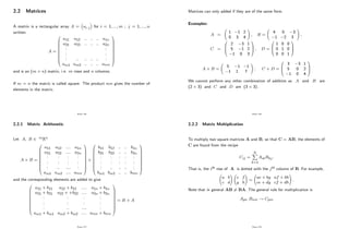
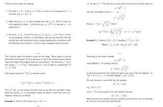
39. the …rst non-zero entry of each row increases row by row.
A matrix A is said to be row equivalent to a matrix B; written A B
if B can be obtained from A from a …nite sequence of operations called
elementary row operations of the form:
[ER1]: Interchange the i th and j th rows: Ri $ Rj
[ER2]:Replace the i th row by itself multiplied by a non-zero constant k :
Ri ! kRi
[ER3]:Replace the i th row by itself plus k times the j th row: Ri ! Ri+kRj
These have no a¤ect on the solution of the of the linear system which gives
the augmented matrix.
Page 152
Examples:
Solve the following linear systems
1.
2x + y 2z = 10
3x + 2y + 2z = 1
5x + 4y + 3z = 4
9
>
=
>
;
Ax = b with
A =
0
B
@
2 1 2
3 2 2
5 4 3
1
C
A and b =
0
B
@
10
1
4
1
C
A
The augmented matrix for this system is
0
B
@
2 1 2
3 2 2
5 4 3
10
1
4
1
C
A
R2!2R2 3R1
R3!2R3 5R1
0
B
@
2 1 2
0 1 10
0 3 16
10
28
42
1
C
A
Page 153
R3!R3 3R2
R1!R1 R2
0
B
@
2 0 12
0 1 10
0 0 14
38
28
42
1
C
A
14z = 42 ! z = 3
y + 10z = 28 ! y = 28 + 30 = 2
x 6z = 19 ! x = 19 18 = 1
Therefore solution is unique with
x =
0
B
@
1
2
3
1
C
A
Page 154
2.
x + 2y 3z = 6
2x y + 4z = 2
4x + 3y 2z = 14
9
>
=
>
;
0
B
@
1 2 3
2 1 4
4 3 2
6
2
14
1
C
A
R2!R2 2R1
R3!R3 4R1
0
B
@
1 2 3
0 5 10
0 5 10
6
10
10
1
C
A
R3!R3 R2
R2!0:5R2
0
B
@
1 2 3
0 1 2
0 0 0
6
2
0
1
C
A
Number of equations is less than number of unknowns.
y 2z = 2 so z = a is a free variable) y = 2 (1 + a)
x + 2y 3z = 6 ! x = 6 2y + 3z = 2 a
Page 155

40. ) x = 2 a; y = 2 (1 + a) ; z = a
Therefore there are many solutions
x =
0
B
@
2 a
2 (1 + a)
a
1
C
A
Page 156
x + 2y 3z = 1
3x y + 2z = 7
5x + 3y 4z = 2
9
>
=
>
;
0
B
@
1 2 3
3 1 2
5 3 4
1
7
2
1
C
A
R2!R2 3R1
R3!R3 5R1
0
B
@
1 2 3
0 7 11
0 7 11
1
10
7
1
C
A
R3!R3 R2
0
B
@
1 2 3
0 7 11
0 0 0
1
10
3
1
C
A
The last line reads 0 = 3: Also middle iteration shows that the second
and third equations are inconsistent.
Hence no solution exists.
Page 157
2.4 Matrix Inverse
The inverse of a matrix A, written A 1; satis…es
AA 1 = A 1A = I:
It may not always exist, but if it does, the solution of the system
Ax = p
is
x = A 1p:
The inverse of the matrix for the special case of a 2 2 matrix
a b
c d
!
=
1
ad bc
d b
c a
!
provided that ad bc 6= 0:
Page 158
The inverse of any n n matrix A is de…ned as
A 1 =
1
jAj
adj A
where adj A =
h
( 1)i+j
Mij
iT
is the adjoint, i.e. we form the matrix of A’
s
cofactors and transpose it.
Mij is the square sub-matrix obtained by "covering the ith row and jth column",
and its determinant is called the Minor of the element aij. The term Aij =
( 1)i+j
Mij is then called the cofactor of aij:
Consider the following example with
A =
0
B
@
1 1 0
1 2 1
0 1 3
1
C
A
So the determinant is given by jAj =
Page 159

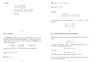
41. ( 1)1+1
A11 jM11j + ( 1)1+2
A12 jM12j + ( 1)1+3
A13 jM13j
= 1
2 1
1 3
1
1 1
0 3
+ 0
1 2
0 1
= (2 3 1 1) (1 3 1 0) + 0 = 5 3
= 2
Here we have expanded about the 1st row - we can do this about any row. If
we expand about the 2nd row - we should still get jAj = 2:
We now calculate the adjoint:
( 1)1+1
M11 = +
2 1
1 3
( 1)1+2
M12 =
1 1
0 3
( 1)1+3
M13 = +
1 2
0 1
( 1)2+1
M21 =
1 0
1 3
( 1)2+2
M22 = +
1 0
0 3
( 1)2+3
M23 =
1 1
0 1
( 1)3+1
M31 = +
1 0
2 1
( 1)3+2
M32 =
1 0
1 1
( 1)3+3
M33 = +
1 1
1 2
Page 160
adj A =
0
B
@
5 3 1
3 3 1
1 1 1
1
C
A
T
We can now write the inverse of A (which is symmetric)
A 1 =
1
2
0
B
@
5 3 1
3 3 1
1 1 1
1
C
A
Elementary row operations (as mentioned above) can be used to simplify a
determinant, as increased numbers of zero entries present, requires less calcu-
lation. There are two important points, however. Suppose the value of the
determinant is jAj ; then:
[ER1]: Ri $ Rj ) jAj ! jAj
[ER2]: Ri ! kRi ) jAj ! k jAj
Page 161
2.5 Orthogonal Matrices
A matrix P is orthogonal if
PPT = PTP =I:
This means that the rows and columns of P are orthogonal and have unit
length. It also means that
P 1 = PT:
In two dimensions, orthogonal matrices have the form
cos sin
sin cos
!
or
cos sin
sin cos
!
for some angle and they correspond to rotations or re‡ections.
Page 162
So rows and columns being orthogonal means row i row j = 0; i.e. they are
perpendicular to each other.
(cos ; sin ) ( sin ; cos ) =
cos sin + sin cos = 0
(cos ; sin ) (sin ; cos ) =
cos sin sin cos = 0
v = (cos ; sin )T
! jvj = cos2 + ( sin )2
= 1
Finally, if P =
cos sin
sin cos
!
then
P 1 =
1
cos2 sin2
| {z }
=1
cos sin
sin cos
!
= PT :
Page 163

42. 2.6 Eigenvalues and Eigenvectors
If A is a square matrix, the problem is to …nd values of (eigenvalue) for
which
Av = v
has a non-trivial vector solution v (eigenvector). We can write the above as
(A I) v= 0:
An N N matrix has exactly N eigenvalues, not all necessarily real or
distinct; they are the roots of the characteristic equation
det (A I) = 0:
Each solution has a corresponding eigenvector v: det (A I) is the char-
acteristic polynomial.
Page 164
The eigenvectors can be regarded as special directions for the matrix A: In
complete generality this is a vast topic. Many Boundary-Value Problems can
be reduced to eigenvalue problems.
We will just look at real symmetric matrices for which A = AT. For these
matrices
The eigenvalues are real;
The eigenvectors corresponding to distinct eigenvalues are orthogonal;
The matrix can be diagonalised: that is, there is an orthogonal matrix
P such that
A = PDPT or PTAP = D
Page 165
where D is diagonal, that is only the entries on the leading diagonal are
non-zero, and these are equal to the eigenvalues of A:
D =
0
B
B
B
B
B
B
@
1 0 0 0 0
0 ... ... ... 0
0 ... ... ... 0
0 ... ... ... 0
0 0 0 0 n
1
C
C
C
C
C
C
A
Example:
A=
0
B
@
3 3 3
3 1 1
3 1 1
1
C
A
then so that the eigenvalues, i.e. the roots of this equation, are 1 = 3;
2 = 2 and 3 = 6:
Page 166
Eigenvectors are now obtained from
0
B
@
3 i 3 3
3 1 i 1
3 1 1 i
1
C
A vi =
0
B
@
0
0
0
1
C
A i = 1; 2; 3
1 = 3 :
0
B
@
6 3 3
3 2 1
3 1 2
1
C
A
0
B
@
x
y
z
1
C
A =
0
B
@
0
0
0
1
C
A
Upon row reduction we have
0
B
@
2 1 1
0 1 1
0 0 0
0
0
0
1
C
A ! y = z; so put z = a
and 2x = y z ! x = ) v1 =
0
B
@
1
1
1
1
C
A
Similarly
Page 167

43. 2 = 2 : v2 =
0
B
@
0
1
1
1
C
A ; 3 = 6 : v3 =
0
B
@
2
1
1
1
C
A
If we take = = = 1 the corresponding eigenvectors are
v1 =
0
B
@
1
1
1
1
C
A ; v2 =
0
B
@
0
1
1
1
C
A ; v3 =
0
B
@
2
1
1
1
C
A
Now normalise these, i.e. jvj = 1: Use b
v = v= jvj for normalised eigen-
vectors
b
v1 =
1
p
3
0
B
@
1
1
1
1
C
A ; b
v2 =
1
p
2
0
B
@
0
1
1
1
C
A ; b
v3 =
1
p
6
0
B
@
2
1
1
1
C
A
Hence
P =
0
B
B
B
@
1
p
3
0 2
p
6
1
p
3
1
p
2
1
p
6
1
p
3
1
p
2
1
p
6
1
C
C
C
A
! PT =
0
B
B
B
@
1
p
3
1
p
3
1
p
3
0 1
p
2
1
p
2
2
p
6
1
p
6
1
p
6
1
C
C
C
A
Page 168
so that
PTAP =
0
B
@
3 0 0
0 2 0
0 0 6
1
C
A
= D:
Page 169
2.6.1 Criteria for invertibility
A system of linear equations is uniquely solvable if and only if the matrix A
is invertible. This in turn is true if any of the following is:
1. If and only if the determinant is non-zero;
2. If and only if all the eigenvalues are non-zero;
3. If (but not only if) it is strictly diagonally dominant.
In practise it takes far too long to work out the determinant. The second
criterion is often useful though, and there are quite quick methods for working
out the eigenvalues. The third method is explained on the next page.
Page 170
A matrix A with entries Aij is strictly diagonally dominant if
jAiij >
X
j6=i
Aij :
That is, the diagonal element in each row is bigger in modulus that the sum
of the moduli of the o¤-diagonal elements in that row. Consider the following
examples:
0
B
@
2 0 1
1 4 2
1 3 6
1
C
A is s.d.d. and so invertible;
0
B
@
1 0 2
2 5 1
3 2 13
1
C
A is not s.d.d. but still invertible;
1 1
1 1
!
is neither s.d.d. nor invertible.
Page 171

44. 3 Di¤erential Equations
3.1 Introduction
2 Types of Di¤erential Equation (D.E)
(i) Ordinary Di¤erential Equation (O.D.E)
Equation involving (ordinary) derivatives
x; y;
dy
dx
;
d 2y
dx2
; ::::::::;
d ny
dxn
(some …xed n)
y is some unknown function of x together with its derivatives, i.e.
Page 172
F x; y; y0; y00; ::::::; y (n) = 0 (1)
Note y4 6= y(4)
Also if y = y (t), where t is time, then we often write
y =
dy
dt
, y =
d 2y
dt2
, ......, y =
d 4y
dt4
Page 173
(ii) Partial Di¤erential Equation (PDE)
Involve partial derivatives, i.e. unknown function dependent on two or more
variables,
e.g.
@u
@t
+
@2u
@x@y
+
@u
@z
u = 0
So here we solving for the unknown function u (x; y; z; t) :
More complicated to solve - better for modelling real-life situations, e.g. …-
nance, engineering & science.
In quant …nance there is no concept of spatial variables, unlike other branches
of mathematics.
Page 174
Order of the highest derivative is the order of the DE
An ode is of degree r if
d ny
dxn
(where n is the order of the derivative) appears
with power r
r Z+ the de…nition of n and r is distinct. Assume that any ode has the
property that each
d`y
dx`
appears in the form
d`y
dx`
!r
!
dny
dxn
!r
order n and degree r.
Page 175

45. Examples:
DE order degree
(1) y0 = 3y 1 1
(2) y0 3
+ 4 sin y = x3 1 3
(3) y(4) 2
+ x2 y(2) 5
+ y0 6
+ y = 0 4 2
(4) y00 =
p
y0 + y + x 2 2
(5) y00 + x y0 3
xy = 0 2 1
Note - example (4) can be written as y00 2
= y0 + y + x
Page 176
We will consider ODE’
s of degree one, and of the form
an (x) dny
dxn + an 1 (x) dn 1y
dxn 1 + :::: + a1 (x) dy
dx + a0 (x) y = g(x)
n
X
i=0
ai (x) y(i) (x) = g (x) (more pedantic)
Note: y(0) (x) - zeroth derivative, i.e. y(x):
This is a Linear ODE of order n, i.e. r = 1 8 (for all) terms. Linear also
because ai (x) not a function of y(i) (x) - else equation is Non-linear.
Page 177
Examples:
DE Nature of DE
(1) 2xy00 + x2y0 (x + 1) y = x2 Linear
(2) yy00 + xy0 + y = 2 a2 = y ) Non-Linear
(3) y00 +
p
y0 + y = x2 Non-Linear * y0
1
2
(4)
d4y
dx4
+ y4 = 0 Non-Linear - y4
Our aim is to solve our ODE either explicitly or by …nding the most general
y (x) satisfying it or implicitly by …nding the function y implicitly in terms of
x, via the most general function g s.t g (x; y) = 0.
Page 178
Suppose that y is given in terms of x and n arbitrary constants of integration
c1, c2, ......., cn.
So e
g (x; c1; c2; :::::::; cn) = 0. Di¤erentiating e
g, n times to get (n + 1)
equations involving
c1; c2; :::::::; cn; x; y; y0; y00; ::::::; y (n).
Eliminating c1; c2; :::::::; cn we get an ODE
e
f x; y; y0; y00; ::::::; y (n) = 0
Page 179

46. Examples:
(1) y = x3 + ce 3x (so 1 constant c)
)
dy
dx
= 3x2 3ce 3x, so eliminate c by taking 3y + y0 = 3x3 + 3x2; i.e.
3x2 (x + 1) + 3y + y0 = 0
(2) y = c1e x + c2e2x (2 constant’
s so di¤erentiate twice)
y0 = c1e x + 2c2e2x ) y00 = c1e x + 4c2e2x
Now
y + y0 = 3c2e2x (a)
y0 + y00 = 6c2e2x (b)
)
and 2(a)=(b) ) 2 y + y0 = y + y00 !
y00 2y0 y = 0.
Page 180
Conversely it can be shown (under suitable conditions) that the general solution
of an nth order ode will involve n arbitrary constants. If we specify values (i.e.
boundary values) of
y; y0; :::::::::::; y(n)
for values of x, then the constants involved may be determined.
Page 181
A solution y = y(x) of (1) is a function that produces zero upon substitution
into the lhs of (1).
Example:
y00 3y0 + 2y = 0 is a 2nd order equation and y = ex is a solution.
y = y0 = y00 = ex - substituting in equation gives ex 3ex + 2ex = 0. So
we can verify that a function is the solution of a DE simply by substitution.
Exercise:
(1) Is y(x) = c1 sin 2x + c2 cos 2x (c1,c2 arbitrary constants) a solution of
y00 + 4y = 0
(2) Determine whether y = x2 1 is a solution of
dy
dx
4
+ y2 = 1
Page 182
3.1.1 Initial & Boundary Value Problems
A DE together with conditions, an unknown function y (x) and its derivatives,
all given at the same value of independent variable x is called an Initial Value
Problem (IVP).
e.g. y00 +2y0 = ex; y ( ) = 1, y0 ( ) = 2 is an IVP because both conditions
are given at the same value x = .
A Boundary Value Problem (BVP) is a DE together with conditions given
at di¤erent values of x, i.e. y00 + 2y0 = ex; y (0) = 1, y (1) = 1.
Here conditions are de…ned at di¤erent values x = 0 and x = 1.
A solution to an IVP or BVP is a function y(x) that both solves the DE and
satis…es all given initial or boundary conditions.
Page 183

47. Exercise: Determine whether any of the following functions
(a) y1 = sin 2x (b) y2 = x (c) y3 = 1
2 sin 2x is a solution of the IVP
y00 + 4y = 0; y (0) = 0; y0 (0) = 1
Page 184
3.2 First Order Ordinary Di¤erential Equations
Standard form for a …rst order DE (in the unknown function y (x)) is
y0 = f (x; y) (2)
so given a 1st order ode
F x; y; y0 = 0
can often be rearranged in the form (2), e.g.
xy0 + 2xy y = 0 ) y0 =
y 2x
x
Page 185
3.2.1 One Variable Missing
This is the simplest case
y missing:
y0 = f (x) solution is y =
Z
f(x)dx
x missing:
y0 = f (y) solution is x =
Z
1
f(y)
dy
Example:
y0 = cos2 y , y =
4
when x = 2
) x =
Z
1
cos2 y
dy =
Z
sec2 y dy ) x = tan y + c ,
c is a constant of integration.
Page 186
This is the general solution. To obtain a particular solution use
y (2) =
4
! 2 = tan
4
+ c ) c = 1
so rearranging gives
y = arctan (x 1)
Page 187

48. 3.2.2 Variable Separable
y0 = g (x) h (y) (3)
So f (x; y) = g (x) h (y) where g and h are functions of x only and y only
in turn. So
dy
dx
= g (x) h (y) !
Z
dy
h (y)
=
Z
g (x) dx + c
c arbitrary constant.
Two examples follow on the next page:
Page 188
dy
dx
=
x2 + 2
y
Z
y dy =
Z
x2 + 2 dx !
y2
2
=
x3
3
+ 2x + c
dy
dx
= y ln x subject to y = 1 at x = e (y (e) = 1)
Z
dy
y
=
Z
ln x dx Recall:
Z
ln x dx = x (ln x 1)
ln y = x (ln x 1) + c ! y = A exp (x ln x x)
A arb. constant
now putting x = e, y = 1 gives A = 1. So solution becomes
y = exp (ln xx) exp ( x) ! y =
xx
ex
) y =
x
e
x
Page 189
3.2.3 Linear Equations
These are equations of the form
y0 + P (x) y = Q (x) (4)
which are similar to (3), but the presence of Q (x) renders this no longer
separable. We look for a function R(x), called an Integrating Factor (I.F)
so that
R(x) y0 + R(x)P (x) y =
d
dx
(R(x)y)
So upon multiplying the lhs of (4), it becomes a derivative of R(x)y, i.e.
R y0 + RPy = Ry0 + R0y
from (4) :
Page 190
This gives RPy = R0y ) R(x)P (x) =
dR
dx
, which is a DE for R which is
separable, hence
Z
dR
R
=
Z
Pdx + c ! ln R =
Z
Pdx + c
So R(x) = K exp (
R
P dx), hence there exists a function R(x) with the
required property. Multiply (4) through by R(x)
R(x)
h
y0 + P(x)y
i
| {z }
= d
dx(R(x)y)
= R(x)Q(x)
d
dx
(Ry) = R(x)Q(x) ! R(x)y =
Z
R(x)Q(x)dx + B
B arb. constant.
We also know the form of R(x) !
yK exp
Z
P dx =
Z
K exp
Z
P dx Q(x)dx + B:
Page 191

49. Divide through by K to give
y exp
Z
P dx =
Z
exp
Z
P dx Q(x)dx + constant.
So we can take K = 1 in the expression for R(x).
To solve y0 + P (x) y = Q (x) calculate R(x) = exp (
R
P dx), which is the
I.F.
Page 192
Examples:
1. Solve y0 1
x
y = x2
In this case c.f (4) gives P(x)
1
x
& Q(x) x2, therefore
I.F R(x) = exp
R 1
x
dx = exp ( ln x) =
1
x
. Multiply DE by
1
x
!
1
x
y0 1
x
y = x )
d
dx
y
x
= x !
Z
d x 1y
=
Z
xdx + c
)
y
x
=
x2
2
+ c ) GS is y =
x3
2
+ cx
Page 193
2. Obtain the general solution of (1 + yex)
dx
dy
= ex
dy
dx
= (1 + yex) e x = e x + y )
dy
dx
y = e x
Which is a linear equation, with P = 1; Q = e x
I.F R(y) = exp
Z
dx = e x
so multiplying DE by I.F
e x y0 y = e 2x !
d
dx
ye x = e 2x )
Z
d ye x =
Z
e 2xdx
ye x =
1
2
e 2x + c ) y = cex 1
2
e x is the GS.
Page 194
3.3 Second Order ODE’
s
Typical second order ODE (degree 1) is
y00 = f x; y; y0
solution involves two arbitrary constants.
3.3.1 Simplest Cases
A y0, y missing, so y00 = f (x)
Integrate wrt x (twice): y =
R
(
R
f (x) dx) dx
Example: y00 = 4x
Page 195

50. GS y =
Z Z
4x dx dx =
Z h
2x2 + C
i
dx =
2x3
3
+ Cx + D
B y missing, so y00 = f y0; x
Put P = y0 ! y00 =
dP
dx
= f (P; x), i.e. P0 = f (P; x) - …rst order ode
Solve once ! P(x)
Solve again ! y(x)
Example: Solve x
d 2y
dx2
+ 2
dy
dx
= x3
Note: A is a special case of B
Page 196
C y0 and x missing, so y00 = f (y)
Put p = y0, then
d 2y
dx2
=
dp
dx
=
dp
dy
dy
dx
= p
dp
dy
= f (y)
So solve 1st order ode
p
dp
dy
= f (y)
which is separable, so
Z
p dp =
Z
f ( y) dy !
Page 197
1
2
p2 =
Z
f (y) dy + const.
Example: Solve y3y00 = 4
) y00 =
4
y3
. Put p = y0 !
d2y
dx2
= p
dp
dy
=
4
y3
)
R
p dp =
Z
4
y3
dy ) p2 =
4
y2
+ D ) p =
q
Dy2 4
y
, so from our
de…nition of p,
dy
dx
=
q
Dy2 4
y
)
Z
dx =
Z
y
q
Dy2 4
dy
Page 198
Integrate rhs by substitution (i.e. u = Dy2 4) to give
x =
q
Dy2 4
D
+ E !
h
D (x E)2
i
= Dy2 4
) GS is Dy2 D2 (x E)2
= 4
D x missing: y00 = f y0; y
Put P = y0, so
d2y
dx2
= P
dP
dy
= f (P; y) - 1st order ODE
Page 199

51. 3.3.2 Linear ODE’
s of Order at least 2
General nth order linear ode is of form:
an (x) y(n) + an 1 (x) y(n 1) + ::::::: + a1 (x) y0 + a0 (x) y = g(x)
Use symbolic notation:
D
d
dx
; Dr d r
dx r
so Dry
d ry
dx r
) arDr ar(x)
d r
dx r
so
arDry = ar(x)
d ry
dx r
Now introduce
L = anDn + an 1Dn 1 + an 2Dn 2 + :::::::::::: + a1D + a0
so we can write a linear ode in the form
L y = g
Page 200
L Linear Di¤erential Operator of order n and its de…nition will be used
throughout.
If g (x) = 0 8x, then L y = 0 is said to be HOMOGENEOUS.
L y = 0 is said to be the homogeneous part of L y = g:
L is a linear operator because as is trivially veri…ed:
(1) L (y1 + y2) = L (y1) + L(y2)
(2) L (cy) = cL (y) c 2 R
GS of Ly = g is given by
y = yc + yp
Page 201
where yc Complimentary Function & yp Particular Integral (or Particular
Solution)
yc is solution of Ly = 0
yp is solution of Ly = g
)
) GS y = yc + yp
Look at homogeneous case Ly = 0. Put s = all solutions of Ly = 0. Then
s forms a vector space of dimension n. Functions y1 (x) ; :::::::::::; yn(x)
are LINEARLY DEPENDENT if 9 1; :::::::::; n 2 R (not all zero) s.t
1y1 (x) + 2y2 (x) + ::::::::::: + nyn(x) = 0
Otherwise yi’
s (i = 1; :::::; n) are said to be LINEARLY INDEPENDENT
(Lin. Indep.) ) whenever
1y1 (x) + 2y2 (x) + ::::::::::: + nyn(x) = 0 8x
then 1 = 2 = ::::::::: = n = 0:
Page 202
FACT:
(1) L nth order linear operator, then 9 n Lin. Indep. solutions y1; :::::; yn
of Ly = 0 s.t GS of Ly = 0 is given by
y = 1y1 + 2y2 + ::::::::::: + nyn i 2 R
1 i n
.
(2) Any n Lin. Indep. solutions of Ly = 0 have this property.
To solve Ly = 0 we need only …nd by "hook or by crook" n Lin. Indep.
solutions.
Page 203

52. 3.3.3 Linear ODE’
s with Constant Coe¢ cients
Consider Homogeneous case: Ly = 0 .
All basic features appear for the case n = 2, so we analyse this.
L y = a
d2y
dx2
+ b
dy
dx
+ cy = 0 a; b; c 2 R
Try a solution of the form y = exp ( x)
L e x = aD2 + bD + c e x
hence a 2 + b + c = 0 and so is a root of the quadratic equation
a 2 + b + c = 0 AUXILLIARY EQUATION (A.E)
Page 204
There are three cases to consider:
(1) b2 4ac > 0
So 1 6= 2 2 R, so GS is
y = c1 exp ( 1x) + c2 exp ( 2x)
c1, c2 arb. const.
(2) b2 4ac = 0
So = 1 = 2 =
b
2a
Page 205
Clearly e x is a solution of L y = 0 - but theory tells us there exist two
solutions for a 2nd order ode. So now try y = x exp ( x)
L xe x = aD2 + bD + c xe x
= a 2 + b + c
| {z }
=0
xe x + (2a + b)
| {z }
=0
e x
= 0
This gives a 2nd solution ) GS is y = c1 exp ( x) + c2x exp ( x), hence
y = (c1 + c2x) exp ( x)
(3) b2 4ac < 0
So 1 6= 2 2 C - Complex conjugate pair = p iq where
p =
b
2a
, q =
1
2a
r
b2 4ac (6= 0)
Page 206
Hence
y = c1 exp (p + iq) x + c2 exp (p iq) x
= c1epxeiq + c2epxe iq = epx c1eiqx + c2e iqx
Eulers identity gives exp ( i ) = cos i sin
Simplifying (using Euler) then gives the GS
y (x) = epx (A cos qx + B sin qx)
Examples:
(1) y00 3y0 4y = 0
Put y = e x to obtain A.E
A.E: 2 3 4 = 0 ! ( 4) ( + 1) = 0 ) = 4 & 1 - 2
distinct R roots
GS y (x) = Ae4x + Be x
Page 207

53. (2) y00 8y0 + 16y = 0
A.E 2 8 + 16 = 0 ! ( 4)2
= 0 ) = 4 , 4 (2 fold root)
’
go up one’
, i.e. instead of y = e x, take y = xe x
GS y (x) = (C + Dx) e4x
(3) y00 3y0 + 4y = 0
A.E: 2 3 + 4 = 0 ! =
3
p
9 16
2
=
3 i
p
7
2
p iq
p =
3
2
, q =
p
7
2
!
y = e
3
2x
a cos
p
7
2
x + b sin
p
7
2
x
!
Page 208
3.4 General nth Order Equation
Consider
Ly = any(n) + an 1y(n 1) + :::::::::: + a1y0 + a0y = 0
then
L anDn + an 1Dn 1 + an 2Dn 2 + ::::::: + a1D + a0
so Ly = 0 and the A.E becomes
an
n + an 1
n 1 + ::::::::::::: + a1 + a0 = 0
Page 209
Case 1 (Basic)
n distinct roots 1; :::::::::; n then e 1x, e 2x, ........, e nx are n Lin. Indep.
solutions giving a GS
y = 1e 1x + 2e 2x + :::::::: + ne nx
i arb.
Case 2
If is a real r fold root of the A.E then e x, xe x, x2e x,.........., xr 1e x
are r Lin. Indep. solutions of Ly = 0, i.e.
y = e x
1 + 2x + 3x2:::::::: + r xr 1
i arb.
Page 210
Case 3
If = p + iq is a r - fold root of the A.E then so is p iq
epx cos qx, xepx cos qx, ..........,xr 1epx cos qx
epx sin qx, xepx sin qx, ............,xr 1epx sin qx
)
! 2r Lin. Indep. solutions of L y = 0
GS y = epx c1 + c2x + c3x2 + :::::::::::: cos qx +
epx C1 + C2x + C3x2 + :::::::::::: sin qx
Page 211

54. Examples: Find the GS of each ODE
(1) y(4) 5y00 + 6y = 0
A.E: 4 5 2 + 6 = 0 ! 2 2 2 3 = 0
So =
p
2 , =
p
3 - four distinct roots
) GS y = Ae
p
2x + Be
p
2x + Ce
p
3x + De
p
3x (Case 1)
(2)
d 6y
dx6
5
d 4y
dx4
= 0
A.E: 6 5 4 = 0 roots: 0; 0; 0; 0;
p
5
GS y = Ae
p
5x + Be
p
5x + C + Dx + Ex2 + Fx3 (* exp(0) = 1)
Page 212
(3)
d 4y
dx4
+ 2
d 2y
dx2
+ y = 0
A.E: 4 + 2 2 + 1 = 2 + 1
2
= 0 = i is a 2 fold root.
Example of Case (3)
y = A cos x + Bx cos x + C sin x + Dx sin x
Page 213
3.5 Non-Homogeneous Case - Method of Undetermined
Coe¢ cients
GS y = C.F + P.I
C.F comes from the roots of the A.E
There are three methods for …nding P.I
(a) "Guesswork" - which we are interested in
(b) Annihilator
(c) D-operator Method
Page 214
(a) Guesswork Method
If the rhs of the ode g (x) is of a certain type, we can guess the form of P.I.
We then try it out and determine the numerical coe¢ cients.
The method will work when g(x) has the following forms
i. Polynomial in x g (x) = p0 + p1x + p2x2 + :::::::::: + pmxm.
ii. An exponential g (x) = Cekx (Provided k is not a root of A.E).
iii. Trigonometric terms, g(x) has the form sin ax, cos ax (Provided ia is
not a root of A.E).
iv. g (x) is a combination of i. , ii. , iii. provided g (x) does not contain part
of the C.F (in which case use other methods).
Page 215

55. Examples:
(1) y00 + 3y0 + 2y = 3e5x
The homogeneous part is the same as in (1), so yc = Ae x + Be 2x. For
the non-homog. part we note that g (x) has the form ekx, so try yp = Ce5x,
and k = 5 is not a solution of the A.E.
Substituting yp into the DE gives
C 52 + 15 + 2 e5x = 3e5x ! C =
1
14
) y = Ae x + Be 2x +
1
14
e5x
Page 216
(2) y00 + 3y0 + 2y = x2
GS y = C.F + P.I = yc + yp
C.F: A.E gives
2 + 3 + 2 = 0 ) = 1; 2 ) yc = ae x + be 2x
P.I Now g(x) = x2,
so try yp = p0 + p1x + p2x2 ! y0
p = p1 + 2p2x ! y00
p = 2p2
Now substitute these in to the DE, ie
2p2 + 3 (p1 + 2p2x) + 2 p0 + p1x + p2x2 = x2 and equate coe¢ cients of
xn
O x2 : 2p2 = 1 ) p2 = 1
2
Page 217
O (x) : 6p2 + 2p1 = 0 ) p1 = 3
2
O x0 : 2p2 + 3p1 + 2p0 = 0 ) p0 = 7
4
) GS y = ae x + be 2x +
7
4
3
2
x +
1
2
x2
Page 218
(3) y00 5y0 6y = cos 3x
A.E: 2 6 = 0 ) = 1, 6 ) yc = e x + e6x
Guided by the rhs, i.e. g (x) is a trigonometric term, we can try yp =
A cos 3x + B sin 3x;and calculate the coe¢ cients A and B:
How about a more sublime approach? Put yp = Re Kei3x for the unknown
coe¢ cient K:
! y0
p = 3 Re iKei3x ! y 00
p = 9 Re Kei3x and substitute into the DE,
dropping Re
( 9 15i 6) Kei3x = ei3x
15 (1 + i) K = 1
15K =
1
1 + i
! K =
1
2
(1 i)
Page 219

56. Hence K = 1
30 (1 i) to give
yp =
1
30
Re (1 i) (cos 3x + i sin 3x)
=
1
30
(cos 3x + i sin 3x i cos 3x + sin 3x)
so general solution becomes
y = e x + e6x 1
30
(cos 3x + sin 3x)
Page 220
3.5.1 Failure Case
Consider the DE y00 5y0 + 6y = e2x, which has a CF given by y (x) =
e2x + e3x. To …nd a PI, if we try yp = Ae2x, we have upon substitution
Ae2x [4 10 + 6] = e2x
so when k (= 2) is also a solution of the C.F , then the trial solution yp =
Aekx fails, so we must seek the existence of an alternative solution.
Page 221
Ly = y00 + ay0 + b = ekx - trial function is normally yp = Cekx:
If k is a root of the A.E then L Cekx = 0 so this substitution does not
work. In this case, we try yp = Cxekx - so ’
go one up’
.
This works provided k is not a repeated root of the A.E, if so try yp = Cx2ekx,
and so forth ....
Page 222
3.6 Linear ODE’
s with Variable Coe¢ cients - Euler Equa-
tion
In the previous sections we have looked at various second order DE’
s with
constant coe¢ cients. We now introduce a 2nd order equation in which the
coe¢ cients are variable in x. An equation of the form
L y = ax2d2y
dx2
+ x
dy
dx
+ cy = g (x)
is called a Cauchy-Euler equation. Note the relationship between the coe¢ cient
and corresponding derivative term, ie an (x) = axn and
d ny
dxn
, i.e. both power
and order of derivative are n.
Page 223

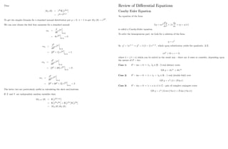
57. The equation is still linear. To solve the homogeneous part, we look for a
solution of the form
y = x
So y0 = x 1 ! y00 = ( 1) x 2 , which upon substitution yields the
quadratic, A.E.
a 2 + b + c = 0
[where b = ( a)] which can be solved in the usual way - there are 3 cases
to consider, depending upon the nature of b2 4ac.
Page 224
Case 1: b2 4ac > 0 ! 1, 2 2 R - 2 real distinct roots
GS y = Ax 1 + Bx 2
Case 2: b2 4ac = 0 ! = 1 = 2 2 R - 1 real (double fold) root
GS y = x (A + B ln x)
Case 3: b2 4ac < 0 ! = i 2 C - pair of complex conjugate
roots
GS y = x (A cos ( ln x) + B sin ( ln x))
Page 225
Example 1 Solve x2y00 2xy0 4y = 0
Put y = x ) y0 = x 1 ) y00 = ( 1) x 2 and substitute
in DE to obtain (upon simpli…cation) the A.E. 2 3 4 = 0 !
( 4) ( + 1) = 0
) = 4 & 1 : 2 distinct R roots. So GS is
y (x) = Ax4 + Bx 1
Example 2 Solve x2y00 7xy0 + 16y = 0
So assume y = x
A.E 2 8 + 16 = 0 ) = 4 , 4 (2 fold root)
’
go up one’
, i.e. instead of y = x , take y = x ln x to give
y (x) = x4 (A + B ln x)
Page 226
Example 3 Solve x2y00 3xy0 + 13y = 0
Assume existence of solution of the form y = x
A.E becomes 2 4 + 13 = 0 ! =
4
p
16 52
2
=
4 6i
2
1 = 2 + 3i, 2 = 2 3i i ( = 2, = 3)
y = x2 (A cos (3 ln x) + B sin (3 ln x))
Page 227

58. 3.6.1 Reduction to constant coe¢ cient
The Euler equation considered above can be reduced to the constant coe¢ cient
problem discussed earlier by use of a suitable transform. To illustrate this simple
technique we use a speci…c example.
Solve x2y00 xy0 + y = ln x
Use the substitution x = et i.e. t = ln x. We now rewrite the the equation
in terms of the variable t, so require new expressions for the derivatives (chain
rule):
dy
dx
=
dy
dt
dt
dx
=
1
x
dy
dt
Page 228
d 2y
dx2
=
d
dx
dy
dx
=
d
dx
1
x
dy
dt
=
1
x
d
dx
dy
dt
1
x2
dy
dt
=
1
x
dt
dx
d
dt
dy
dt
1
x2
dy
dt
=
1
x2
d2y
dt2
1
x2
dy
dt
) the Euler equation becomes
x2 1
x2
d2y
dt2
1
x2
dy
dt
!
x
1
x
dy
dt
+ y = t !
y00 (t) 2y0 (t) + y = t
The solution of the homogeneous part , ie C.F. is yc = et (A + Bt) :
The particular integral (P.I.) is obtained by using yp = p0 + p1t to give
yp = 2 + t
Page 229
The GS of this equation becomes
y (t) = et (A + Bt) + 2 + t
which is a function of t . The original problem was y = y (x), so we use our
transformation t = ln x to get the GS
y = x (A + B ln x) + 2 + ln x.
Page 230
3.7 Partial Di¤erential Equations
The formation (and solution) of PDE’
s forms the basis of a large number
of mathematical models used to study physical situations arising in science,
engineering and medicine.
More recently their use has extended to the modelling of problems in …nance
and economics.
We now look at the second type of DE, i.e. PDE’
s. These have partial
derivatives instead of ordinary derivatives.
One of the underlying equations in …nance, the Black-Scholes equation for the
price of an option V (S; t) is an example of a linear PDE
@V
@t
+
1
2
2S2@2V
@S2
+ (r D) S
@V
@S
rV = 0
Page 231

59. providing ; D; r are not functions of V or any of its derivatives.
If we let u = u (x; y) ; then the general form of a linear 2nd order PDE is
A
@2u
@x2
+ B
@2u
@x@y
+ C
@2u
@y2
+ D
@u
@x
+ E
@u
@y
+ Fu = G
where the coe¢ cients A; ::::; G are functions of x & y:
When
G (x; y) =
(
0 (1) is homogeneous
non-zero (1) is non-homogeneous
hyperbolic B2 4AC > 0
parabolic B2 4AC = 0
elliptic B2 4AC < 0
Page 232
In the context of mathematical …nance we are only interested in the 2nd type,
i.e. parabolic.
There are several methods for obtaining solutions of PDE’
s.
We look at a simple (but useful) technique:
Page 233
3.7.1 Method of Separation of Variables
Without loss of generality, we solve the one-dimensional heat equation
@u
@t
= c2@2u
@x2
(*)
for the unknown function u (x; t) :
In this method we assume existence of a solution which is a product of a
function of x (only) and a function of y (only). So the form is
u (x; t) = X (x) T (t) :
We substitute this in (*), so
@u
@t
=
@
@t
(XT) = XT0
@2u
@x2
=
@
@x
@
@x
(XT) =
@
@x
X0T = X00T
Page 234
Therefore (*) becomes
X T 0 = c2X 00 T
dividing through by c2X T gives
T0
c2T
=
X00
X
:
The RHS is independent of t and LHS is independent of x:
So each equation must be a constant. The convention is to write this constant
as 2 or 2:
There are possible cases:
Case 1: 2 > 0
T 0
c2T
=
X 00
X
= 2 leading to
T 0 2c2T = 0
X 00 2X = 0
)
Page 235

60. which have solutions, in turn
T (t) = k exp c2 2t
X (x) = A cosh ( x) + B sinh ( x)
)
So solution is
u (x; t) = X T = k exp c2 2t fA cosh ( x) + B sinh ( x)g
Therefore u = exp c2 2t f cosh ( x) + sinh ( x)g
( = Ak; = Bk)
Page 236
Case 2: 2 < 0
T 0
c2T
=
X 00
X
= 2 which gives
T 0 + 2c2T = 0
X 00 + 2X = 0
)
resulting in the solutions
T = k exp c2 2t
X = A cos ( x) + B sin ( x)
)
respectively.
Hence
u (x; t) = exp c2 2t f cos ( x) + sin ( x)g
where = kA; = kB :
Page 237
Case 3: 2 = 0
T 0 = 0
X 00 = 0
)
!
T (t) = e
A
X = e
Bx + e
C
)
which gives the simple solution
u (x; y) = b
Ax + b
C
where b
A = e
A e
B; b
C = e
B e
C :
Page 238

61. CERTIFICATE IN
FINANCE
CQF
Certificate in Quantitative Finance
Subtext t here
1 PROBABILITY
1 Probability
1.1 Preliminaries
• An experiment is a repeatable process that gives
rise to a number of outcomes.
• An event is a collection (or set) of one or more out-
comes.
• An sample space is the set of all possible outcomes
of an experiment, often denoted Ω.
Example
In an experiment a dice is rolled and the number ap-
pearing on top is recorded.
Thus
Ω = {1, 2, 3, 4, 5, 6}
If E1, E2, E3 are the events even, odd and prime occur-
ring, then
E1 ={2, 4, 6}
E2 ={1, 3, 5}
E3 ={2, 3, 5}
2

62. 1.1 Preliminaries 1 PROBABILITY
1.1.1 Probability Scale
Probability of an Event E occurring i.e. P(E) is less
than or equal to 1 and greater than or equal to 0.
0 ≤ P(E) ≤ 1
1.1.2 Probability of an Event
The probability of an event occurring is defined as:
P(E) =
The number of ways the event can occur
Total number of outcomes
Example
A fair dice is tossed. The event A is defined as the
number obtained is a multiple of 3. Determine P(A)
Ω ={1, 2, 3, 4, 5, 6}
A ={3, 6}
∴ P(A) =
2
6
1.1.3 The Complimentary Event E0
An event E occurs or it does not. If E is the event then
E0
is the complimentary event, i.e. not E where
P(E0
) = 1 − P(E)
3
1.2 Probability Diagrams 1 PROBABILITY
1.2 Probability Diagrams
It is useful to represent problems diagrammatically. Three
useful diagrams are:
• Sample space or two way table
• Tree diagram
• Venn diagram
Example
Two dice are thrown and their numbers added to-
gether. What is the probability of achieving a total of
8?
P(8) =
5
36
Example
A bag contains 4 red, 5 yellow and 11 blue balls. A
ball is pulled out at random, its colour noted and then
4

63. 1.2 Probability Diagrams 1 PROBABILITY
replaced. What is the probability of picking a red and a
blue ball in any order.
P(Red and Blue) or P(Blue and Red) =
4
20
×
11
20
+
11
20
×
4
20
=
11
50
Venn Diagram
A Venn diagram is a way of representing data sets or
events. Consider two events A and B. A Venn diagram
to represent these events could be:
• A ∪ B ”A or B”
5
1.2 Probability Diagrams 1 PROBABILITY
• A ∩ B ”A and B”
Addition Rule:
P(A ∪ B) = P(A) + P(B) − P(A ∩ B)
or
P(A ∩ B) = P(A) + P(B) − P(A ∪ B)
Example
In a class of 30 students, 7 are in the choir, 5 are in
the school band and 2 students are in the choir and the
school band. A student is chosen at random from the
class. Find:
a) The probability the student is not in the band
b) The probability the student is not in the choir nor in
the band
6

64. 1.2 Probability Diagrams 1 PROBABILITY
P(not in band) =
5 + 20
30
=
25
30
=
5
6
P(not in either) =
20
30
=
2
3
Example
A vet surveys 100 of her clients, she finds that:
(i) 25 own dogs
(ii) 53 own cats
(iii) 40 own tropical fish
(iv) 15 own dogs and cats
(v) 10 own cats and tropical fish
7
1.2 Probability Diagrams 1 PROBABILITY
(vi) 11 own dogs and tropical fish
(vii) 7 own dogs, cats and tropical fish
If she picks a client at random, Find:
a) P(Owns dogs only)
b) P(Does not own tropical fish)
c) P(Does not own dogs, cats or tropical fish)
P(Dogs only) =
6
100
P(Does not own tropical fish) =
6 + 8 + 35 + 11
100
=
60
100
P(Does not own dogs, cats or tropical fish) =
11
100
8

65. 1.3 Conditional Probability 1 PROBABILITY
1.3 Conditional Probability
The probability of an event B may be different if you
know that a dependent event A has already occurred.
Example
Consider a school which has 100 students in its sixth
form. 50 students study mathematics, 29 study biology
and 13 study both subjects. You walk into a biology class
and select a student at random. What is the probability
that this student also studies mathematics?
P(study maths given they study biology) = P(M|B) =
13
29
In general, we have:
9
1.3 Conditional Probability 1 PROBABILITY
P(A|B) =
P(A ∩ B)
P(B)
or, Multiplication Rule:
P(A ∩ B) = P(A|B) × P(B)
Example
You are dealt exactly two playing cards from a well
shuffled standard 52 card deck. What is the probability
that both your cards are Kings ?
Tree Diagram!
P(K ∩ K) =
4
52
×
3
51
=
1
221
=≈ 0.5%
or
P(K∩K) = P(2nd is King | first is king)×P(first is king) =
3
51
×
4
52
We know,
P(A ∩ B) = P(B ∩ A)
10

66. 1.3 Conditional Probability 1 PROBABILITY
so
P(A ∩ B) = P(A|B) × P(B)
P(B ∩ A) = P(B|A) × P(A)
i.e.
P(A|B) × P(B) = P(B|A) × P(A)
or
Bayes’ Theorem:
P(B|A) =
P(A|B) × P(B)
P(A)
Example
You have 10 coins in a bag. 9 are fair and 1 is double
headed. If you pull out a coin from the bag and do not
examine it. Find:
1. Probability of getting 5 heads in a row
2. Probability that if you get 5 heads the you picked
the double headed coin
11
1.3 Conditional Probability 1 PROBABILITY
P(5heads) = P(5heads|N) × P(N) + P(5heads|H) × P(H)
=
1
32
×
9
10
+
1 ×
1
10
=
41
320
≈ 13%
P(H|5heads) =
P(5heads|H) × P(H)
P(5heads)
=
1 × 1
10
41
320
=
320
410
≈ 78%
12

67. 1.4 Mutually exclusive and Independent events 1 PROBABILITY
1.4 Mutually exclusive and Independent
events
When events can not happen at the same time, i.e. no
outcomes in common, they are called mutually exclu-
sive. If this is the case, then
P(A ∩ B) = 0
and the addition rule becomes
P(A ∪ B) = P(A) + P(B)
Example
Two dice are rolled, event A is ’the sum of the out-
comes on both dice is 5’ and event B is ’the outcome on
each dice is the same’
When one event has no effect on another event, the
two events are said to be independent, i.e.
P(A|B) = P(A)
and the multiplication rule becomes
P(A ∩ B) = P(A) × P(B)
13
1.5 Two famous problems 1 PROBABILITY
Example
A red dice and a blue dice are rolled, if event A is ’the
outcome on the red dice is 3’ and event B ’is the outcome
on the blue dice is 3’ then events A and B are said to be
independent.
1.5 Two famous problems
• Birthday Problem - What is the probability that
at least 2 people share the same birthday
• Monty Hall Game Show - Would you swap ?
14

68. 1.6 Random Variables 1 PROBABILITY
1.6 Random Variables
1.6.1 Notation
Random Variables X, Y, Z
Observed Variables x, y, z
1.6.2 Definition
Outcomes of experiments are not always numbers, e.g.
two heads appearing; picking an ace from a deck of cards.
We need some way of assigning real numbers to each ran-
dom event. Random variables assign numbers to events.
Thus a random variable (RV) X is a function which
maps from the sample space Ω to the number line.
Example
let X = the number facing up when a fair dice is rolled,
or let X represent the outcome of a coin toss, where
X =
1 if heads
0 if tails
1.6.3 Types of Random variable
1. Discrete - Countable outcomes, e.g. roll of a dice,
rain or no rain
2. Continuous - Infinite number of outcomes, e.g. exact
amount of rain in mm
15
1.7 Probability Distributions 1 PROBABILITY
1.7 Probability Distributions
Depending on whether you are dealing with a discrete
or continuous random variable will determine how you
define your probability distribution.
1.7.1 Discrete distributions
When dealing with a discrete random variable we de-
fine the probability distribution using a probaility mass
fucntion or simply a probability function.
Example
The RV X is defined as’ the sum of scores shown by
two fair six sided dice’. Find the probability distribution
of X
A sample space diagram for the experiment is:
The distribution can be tabulated as:
x 2 3 4 5 6 7 8 9 10 11 12
P(X = x) 1
36
2
36
3
36
4
36
5
36
6
36
5
36
4
36
3
36
2
36
1
36
16

69. 1.7 Probability Distributions 1 PROBABILITY
or can be represented on a graph as
1.7.2 Continuous Distributions
As continuous random variables can take any value, i.e an
infinite number of values, we must define our probability
distribution differently.
For a continuous RV the probability of getting a spe-
cific value is zero, i.e
P(X = x) = 0
and so just as we go from bar charts to histograms when
representing discrete and continuous data, we must use a
probability density function (PDF) when describing the
probability distribution of a continuous RV.
17
1.7 Probability Distributions 1 PROBABILITY
P(a X b) =
Z b
a
f(x)dx
Properties of a PDF:
• f(x) ≥ 0 since probabilities are always positive
•
R +∞
∞ f(x)dx = 1
• P(a X b) =
R b
a f(x)dx
Example
The random variable X has the probability density
function:
f(x) =



k 1 x 2
k(x − 1) 2 ≤ x ≤ 4
0 otherwise
18

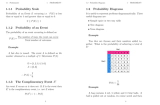
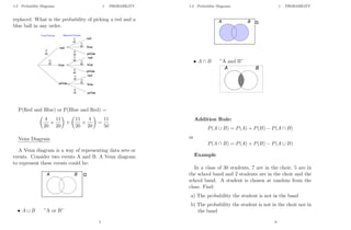
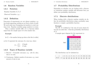
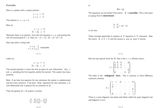
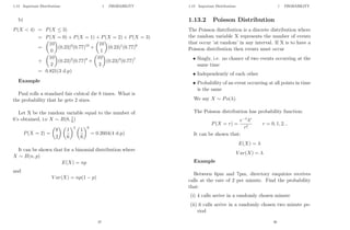
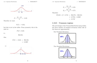
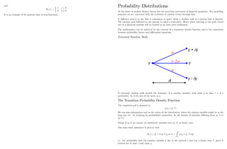
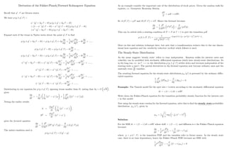
70. 1.7 Probability Distributions 1 PROBABILITY
a) Find k and Sketch the probability distribution
b) Find P(X ≤ 1.5)
a)
Z +∞
∞
f(x)dx = 1
1 =
Z 2
1
kdx +
Z 4
2
k(x − 1)dx
1 = [kx]2
1 +
kx2
2
− kx
4
2
1 = 2k − k + [(8k − 4k) − (2k − 2k)]
1 = 5k
∴ k =
1
5
19
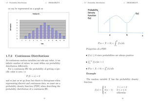
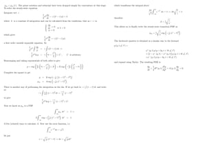
1.8 Cumulative Distribution Function 1 PROBABILITY
b)
P(X ≤ 1.5) =
Z 1.5
1
1
5
dx
=
hx
5
i1.5
1
=
1
10
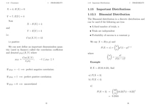
1.8 Cumulative Distribution Function
The CDF is an alternative function for summarising a
probability distribution. It provides a formula for P(X ≤
x), i.e.
F(x) = P(X ≤ x)
1.8.1 Discrete Random variables
Example
Consider the probability distribution
x 1 2 3 4 5 6
P(X = x) 1
2
1
4
1
8
1
16
1
32
1
32
F(X) = P(X ≤ x)
Find:
a) F(2) and
b) F(4.5)
20

71. 1.8 Cumulative Distribution Function 1 PROBABILITY
a)
F(2) = P(X ≤ 2) = P(X = 1) + P(X = 2)
=
1
2
+
1
4
=
3
4
b)
F(4.5) = P(X ≤ 4.5) = P(X ≤ 4)
=
1
16
+
1
8
+
1
4
+
1
2
=
15
16
1.8.2 Continuous Random Variable
For continuous random variables
F(X) = P(X ≤ x) =
Z x
−∞
f(x)dx
or
f(x) =
d
dx
F(x)
Example
A PDF is defined as
f(x) =
3
11(4 − x2
) 0 ≤ x ≤ 1
0 otherwise
Find the CDF
21
1.8 Cumulative Distribution Function 1 PROBABILITY
Consider:
From −∞ to 0: F(x) = 0
From 1 to ∞: F(x) = 1
From 0 to 1 :
22

72. 1.8 Cumulative Distribution Function 1 PROBABILITY
F(x) =
Z x
0
3
11
(4 − x2
)dx
=
3
11
4x −
x3
3
x
0
=
3
11
4x −
x3
3
i.e.
F(x) =





0 x 0
3
11
h
4x − x3
3
i
0 ≤ x ≤ 1
1 x 1
Example
A CDF is defined as:
F(x) =



0 x 1
1
12
x2
+ 2x − 3
1 ≤ x ≤ 3
1 x 3
a) Find P(1.5 ≤ x ≤ 2.5)
b) Find f(x)
a)
P(1.5 ≤ x ≤ 2.5) = F(2.5) − F(1.5)
=
1
12
(2.52
+ 2(2.5) − 3) −
1
12
(1.52
+ 2(1.5) − 3)
= 0.5
23
1.9 Expectation and Variance 1 PROBABILITY
b)
f(x) =
d
dx
F(x)
f(x) =
1
6(x + 1) 1 ≤ x ≤ 3
0 otherwise
1.9 Expectation and Variance
The expectation or expected value of a random variable
X is the mean µ (measure of center), i.e.
E(X) = µ
The variance of a random variables X is a measure of
dispersion and is labeled σ2
, i.e.
V ar(X) = σ2
1.9.1 Discrete Random variables
For a discrete random variable
E(X) =
X
allx
xP(X = x)
Example
Consider the probability distribution
x 1 2 3 4
P(X = x) 1
2
1
4
1
8
1
8
then
24

73. 1.9 Expectation and Variance 1 PROBABILITY
E(X) = (1 ×
1
2
) + (2 ×
1
4
) + (3 ×
1
8
) + (4 ×
1
8
)
=
15
8
25
1.9 Expectation and Variance 1 PROBABILITY
Aside
What is Variance?
Variance =
P
(x − µ)2
n
=
P
x2
n
− µ2
Standard deviation =
rP
(x − µ)2
n
=
rP
x2
n
− µ2
26

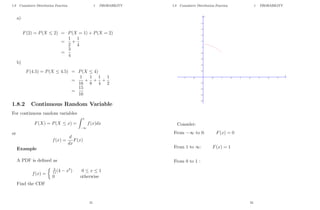
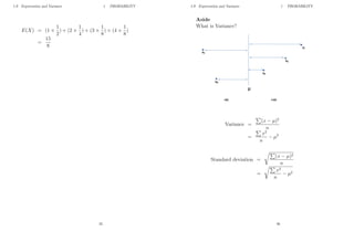
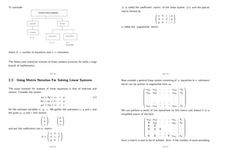
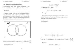
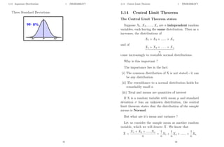
74. 1.9 Expectation and Variance 1 PROBABILITY
For a discrete random variable
V ar(X) = E(X2
) − [E(X)]2
Now, for previous example
E(X2
) = 12
×
1
2
+ 22
×
1
4
+ 32
× 18 + 42
×
1
8
E(X) =
15
18
∴ V ar(X) =
71
64
= 1.10937...
Standard Deviation = 1.05(3s.f)
1.9.2 Continuous Random Variables
For a continuous random variable
E(X) =
Z
allx
xf(x)dx
and
V ar(X) = E(X2
) − [E(X)]2
=
Z
allx
x2
f(x)dx −
Z
allx
xf(x)dx
2
Example
if
f(x) =
3
32(4x − x2
) 0 ≤ x ≤ 4
0 otherwise
27
1.9 Expectation and Variance 1 PROBABILITY
Find E(X) and V ar(X)
E(X) =
Z 4
0
x.
3
32
(4x − x2
)dx
=
3
32
Z 4
0
4x − x2
dx
=
3
32
4x3
3
−
x4
4
4
0
=
3
32
4(4)3
3
−
44
4
− (0)
= 2
V ar(X) = E(X2
) − [E(X)]2
=
Z 4
0
x2
.
3
32
(4x − x2
)dx − 22
=
3
32
4x4
4
−
x5
5
4
0
− 4
=
3
32
44
−
45
5
− 4
=
4
5
28

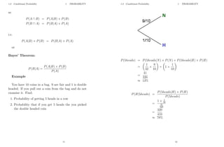
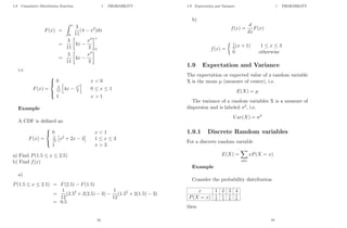
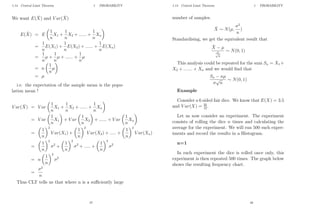
75. 1.10 Expectation Algebra 1 PROBABILITY
1.10 Expectation Algebra
Suppose X and Y are random variables and a,b and c
are constants. Then:
• E(X + a) = E(X) + a
• E(aX) = aE(X)
• E(X + Y ) = E(X) + E(Y )
• V ar(X + a) = V ar(X)
• V ar(aX) = a2
V ar(X)
• V ar(b) = 0
If X and Y are independent, then
• E(XY ) = E(X)E(Y )
• V ar(X + Y ) = V ar(X) + V ar(Y )
29
1.11 Moments 1 PROBABILITY
1.11 Moments
The first moment is E(X) = µ
The nth
moment is E(Xn
) =
R
allx xn
f(x)dx
We are often interested in the moments about the
mean, i.e. central moments.
The 2nd
central moment about the mean is called the
variance E[(X − µ)2
] = σ2
The 3rd
central moment is E[(X − µ)3
]
So we can compare with other distributions, we scale
with σ3
and define Skewness.
Skewness =
E[(X − µ)3
]
σ3
This is a measure of asymmetry of a distribution. A
distribution which is symmetric has skew of 0. Negative
values of the skewness indicate data that are skewed to
the left, where positive values of skewness indicate data
skewed to the right.
30

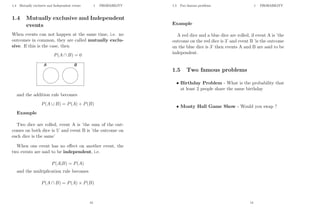
76. 1.11 Moments 1 PROBABILITY
The 4th
normalised central moment is called Kurtosis
and is defined as
Kurtosis =
E[(X − µ)4
]
σ4
A normal random variable has Kurtosis of 3 irrespec-
tive of its mean and standard deviation. Often when
comparing a distribution to the normal distribution, the
measure of excess Kurtosis is used, i.e. Kurtosis of
distribution −3.
Intiution to help understand Kurtosis
Consider the following data and the effect on the Kur-
tosis of a continuous distribution.
xi µ ± σ :
The contribution to the Kurtosis from all data points
within 1 standard deviation from the mean is low since
(xi − µ)4
σ4
1
e.g consider
x1 = µ +
1
2
σ
then
(x1 − µ)4
σ4
=
1
2
4
σ4
σ4
=
1
2
4
=
1
16
xi µ ± σ :
31
1.11 Moments 1 PROBABILITY
The contribution to the Kurtosis from data points
greater than 1 standard deviation from the mean will
be greater the further they are from the mean.
(xi − µ)4
σ4
1
e.g consider
x1 = µ + 3σ
then
(x1 − µ)4
σ4
=
(3σ)4
σ4
= 81
This shows that a data point 3 standard deviations
from the mean would have a much greater effect on the
Kurtosis than data close to the mean value. Therefore,
if the distribution has more data in the tails, i.e. fat tails
then it will have a larger Kurtosis.
Thus Kurtosis is often seen as a measure of how ’fat’
the tails of a distribution are.
If a random variable has Kurtosis greater than 3 is
is called Leptokurtic, if is has Kurtosis less than 3 it is
called platykurtic
Leptokurtic is associated with PDF’s that are simul-
taneously peaked and have fat tails.
32

77. 1.11 Moments 1 PROBABILITY
33
1.12 Covariance 1 PROBABILITY
1.12 Covariance
The covariance is useful in studying the statistical de-
pendence between two random variables. If X and Y
are random variables, then theor covariance is defined
as:
Cov(X, Y ) = E [(X − E(X))(Y − E(Y ))]
= E(XY ) − E(X)E(Y )
Intuition
Imagine we have a single sample of X and Y, so that:
X = 1, E(X) = 0
Y = 3, E(Y ) = 4
Now
X − E(X) = 1
and
Y − E(Y ) = −1
i.e.
Cov(X, Y ) = −1
So in this sample when X was above its expected value
and Y was below its expected value we get a negative
number.
Now if we do this for every X and Y and average
this product, we should find the Covariance is negative.
What about if:
34

78. 1.12 Covariance 1 PROBABILITY
X = 4, E(X) = 0
Y = 7, E(Y ) = 4
Now
X − E(X) = 4
and
Y − E(Y ) = 3
i.e.
Cov(X, Y ) = 12
i.e positive
We can now define an important dimensionless quan-
tity (used in finance) called the correlation coefficient
and denoted ρXY (X, Y ) where
ρXY =
Cov(X, Y )
σXσY
; −1 ≤ ρXY ≤ 1
If ρXY = −1 =⇒ perfect negative correlation
If ρXY = 1 =⇒ perfect positive correlation
If ρXY = 0 =⇒ uncorrelated
35
1.13 Important Distributions 1 PROBABILITY
1.13 Important Distributions
1.13.1 Binomial Distribution
The Binomial distribution is a discrete distribution and
can be used if the following are true.
• A fixed number of trials, n
• Trials are independent
• Probability of success is a constant p
We say X ∼ B(n, p) and
P(X = x) =
n
x
px
(1 − p)n−x
where
n
x
=
n!
x!(n − x)!
Example
If X ∼ B(10, 0.23), find
a) P(X = 3)
b) P(X 4)
a)
P(X = 3) =
10
3
(0.23)3
(1 − 0.23)7
= 0.2343
36

79. 1.13 Important Distributions 1 PROBABILITY
b)
P(X 4) = P(X ≤ 3)
= P(X = 0) + P(X = 1) + P(X = 2) + P(X = 3)
=
10
0
(0.23)0
(0.77)10
+
10
1
(0.23)1
(0.77)9
+
10
2
(0.23)2
(0.77)8
+
10
3
(0.23)3
(0.77)7
= 0.821(3 d.p)
Example
Paul rolls a standard fair cubical die 8 times. What is
the probability that he gets 2 sixes.
Let X be the random variable equal to the number of
6’s obtained, i.e X ∼ B(8, 1
6)
P(X = 2) =
8
2
1
6
2
1
6
6
= 0.2604(4 d.p)
It can be shown that for a binomial distribution where
X ∼ B(n, p)
E(X) = np
and
V ar(X) = np(1 − p)
37
1.13 Important Distributions 1 PROBABILITY
1.13.2 Poisson Distribution
The Poisson distribution is a discrete distribution where
the random variable X represents the number of events
that occur ’at random’ in any interval. If X is to have a
Poisson distribution then events must occur
• Singly, i.e. no chance of two events occurring at the
same time
• Independently of each other
• Probability of an event occurring at all points in time
is the same
We say X ∼ Po(λ).
The Poisson distribution has probability function:
P(X = r) =
e−λ
λr
r!
r = 0, 1, 2...
It can be shown that:
E(X) = λ
V ar(X) = λ
Example
Between 6pm and 7pm, directory enquiries receives
calls at the rate of 2 per minute. Find the probability
that:
(i) 4 calls arrive in a randomly chosen minute
(ii) 6 calls arrive in a randomly chosen two minute pe-
riod
38

80. 1.13 Important Distributions 1 PROBABILITY
(i) Let X be the number of call in 1 minute, so
λ = 2, i.e. E(X) = 2
and
X ∼ Po(2) =
e−2
2r
r!
P(X = 4) =
e−2
24
4!
= 0.090(3 d.p)
(ii) Let Y be the number of calls in 2 minutes, so
λ = 4, i.e. E(Y ) = 4
and
P(Y = 6) =
e−4
46
6!
= 0.104(3 d.p)
39
1.13 Important Distributions 1 PROBABILITY
1.13.3 Normal Distribution
The Normal distribution is a continuous distribution.
This is the most important distribution. If X is a ran-
dom variable that follows the normal distribution we say:
X ∼ N(µ, σ2
)
where
E(X) = µ
V ar(X) = σ2
and the PDF is described as
PDF = f(x) =
1
σ
√
2π
e
(x−µ)2
2σ2
i.e.
P(X ≤ x) =
Z x
−∞
1
σ
√
2π
e
(s−µ)2
2σ2
ds
The Normal distribution is symmetric and area under
the graph equals 1, i.e.
Z +∞
−∞
1
σ
√
2π
e
(x−µ)2
2σ2
dx = 1
40

81. 1.13 Important Distributions 1 PROBABILITY
To find the probabilities we must integrate under f(x),
this is not easy to do and requires numerical methods.
In order to avoid this numerical calculation we define
a standard normal distribution, for which values have
already been documented.
The Standard Normal distribution is just a transfor-
mation of the Normal distribution.
1.13.4 Standard Normal distribution
We define a standard normal random variable by Z,
where Z ∼ N(0, 1), i.e.
E(Z) = 0
V ar(Z) = 1
thus the PDF is
φ(z) =
1
√
2π
e
−z2
2
and
Φ(z) =
Z z
−∞
1
√
2π
e
−s2
2 ds
41
1.13 Important Distributions 1 PROBABILITY
To transform a Normal distribution into a Standard
Normal distribution, we use:
Z =
X − µ
σ
Example
Given X ∼ N(12, 16) find:
a) P(X 14)
b) P(X 11)
c) P(13 X 15)
a)
Z =
X − µ
σ
=
14 − 12
4
= 0.5
Therefore we want
P(Z ≤ 0.5) = Φ(0.5)
= 0.6915
(from tables)
b)
42

82. 1.13 Important Distributions 1 PROBABILITY
Z =
11 − 12
4
= −0.25
Therefore we want
P(Z −0.25)
but this is not in the tables. From symmetry this is the
same as
P(Z 0.25)
i.e.
Φ(0.25)
thus
P(Z −0.25) = Φ(0.25)
= 0.5987
c)
43
1.13 Important Distributions 1 PROBABILITY
Z1 =
13 − 12
4
= 0.25
Z2 =
15 − 12
4
= 0.75
Therefore
P(0.25 Z 0.75) = Φ(0.75) − Φ(0.25)
= 0.7734 − 0.5987
= 0.1747
1.13.5 Common regions
The percentages of the Normal Distribution lying within
the given number of standard deviations either side of
the mean are approximately:
One Standard Deviation:
Two Standard Deviations:
44

83. 1.13 Important Distributions 1 PROBABILITY
Three Standard Deviations:
45
1.14 Central Limit Theorem 1 PROBABILITY
1.14 Central Limit Theorem
The Central Limit Theorem states:
Suppose X1, X2, ......, Xn are n independent random
variables, each having the same distribution. Then as n
increases, the distributions of
X1 + X2 + ...... + Xn
and of
X1 + X2 + ...... + Xn
n
come increasingly to resemble normal distributions.
Why is this important ?
The importance lies in the fact:
(i) The common distribution of X is not stated - it can
be any distribution
(ii) The resemblance to a normal distribution holds for
remarkably small n
(iii) Total and means are quantities of interest
If X is a random variable with mean µ and standard
devaition σ fom an unknown distribution, the central
limit theorem states that the distribution of the sample
means is Normal.
But what are it’s mean and variance ?
Let us consider the sample mean as another random
variable, which we will denote X̄. We know that
X̄ =
X1 + X2 + ......Xn
n
=
1
n
X1 +
1
n
X2 + ...... +
1
n
Xn
46

84. 1.14 Central Limit Theorem 1 PROBABILITY
We want E(X̄) and V ar(X̄)
E(X̄) = E
1
n
X1 +
1
n
X2 + ...... +
1
n
Xn
=
1
n
E(X1) +
1
n
E(X2) + ...... +
1
n
E(Xn)
=
1
n
µ +
1
n
µ + ...... +
1
n
µ
= n
1
n
µ
= µ
i.e. the expectation of the sample mean is the popu-
lation mean !
V ar(X̄) = V ar
1
n
X1 +
1
n
X2 + ...... +
1
n
Xn
= V ar
1
n
X1
+ V ar
1
n
X2
+ ...... + V ar
1
n
Xn
=
1
n
2
V ar(X1) +
1
n
2
V ar(X2) + ..... +
1
n
2
V ar(Xn)
=
1
n
2
σ2
+
1
n
2
σ2
+ ..... +
1
n
2
σ2
= n
1
n
2
σ2
=
σ2
n
Thus CLT tells us that where n is a sufficiently large
47
1.14 Central Limit Theorem 1 PROBABILITY
number of samples.
X̄ ∼ N(µ,
σ2
n
)
Standardising, we get the equivalent result that
X̄ − µ
σ
√
n
∼ N(0, 1)
This analysis could be repeated for the sum Sn = X1 +
X2 + ....... + Xn and we would find that
Sn − nµ
σ
√
n
∼ N(0, 1)
Example
Consider a 6 sided fair dice. We know that E(X) = 3.5
and V ar(X) = 35
12.
Let us now consider an experiment. The experiment
consists of rolling the dice n times and calculating the
average for the experiment. We will run 500 such exper-
iments and record the results in a Histogram.
n=1
In each experiment the dice is rolled once only, this
experiment is then repeated 500 times. The graph below
shows the resulting frequency chart.
48

85. 1.14 Central Limit Theorem 1 PROBABILITY
This clearly resembles a uniform distribution (as ex-
pected).
Let us now increase the number of rolls, but continue
to carry out 500 experiments each time and see what
happens to the distribution of X̄
n=5
49
1.14 Central Limit Theorem 1 PROBABILITY
n=10
n=30
We can see that even for small sample sizes (number
of dice rolls), our resulting distribution begins to look
more like a Normal distribution. we can also note that
as n increases our distribution begins to narrow, i.e. the
variance becomes smaller σ2
n , but the mean remains the
same µ.
50

86. 2 STATISTICS
2 Statistics
2.1 Sampling
So far we have been dealing with populations, however
sometimes the population is too large to be able to anal-
yse and we need to use a sample in order to estimate the
population parameters, i.e. mean and variance.
Consider a population of N data points and a sample
taken from this population of n data points.
We know that the mean and variance of a population
are given by:
population mean, µ =
PN
i=1 xi
N
and
population variance, σ2
=
PN
i=1 (xi − x̄)2
N
51
2.1 Sampling 2 STATISTICS
But how can we use the sample to estimate our pop-
ulation parameters?
First we define an unbiased estimator. An unbiased
estimator is when the expected value of the estimator is
exactly equal to the corresponding population parame-
ter, i.e.
if x̄ is the sample mean then the unbiased estimator is
E(x̄) = µ
where the sample mean is given by:
x̄ =
PN
i=1 xi
n
If S2
is the sample variance, then the unbiased esti-
mator is
E(S2
) = σ2
where the sample variance is given by:
S2
=
Pn
i=1 (xi − x̄)2
n − 1
2.1.1 Proof
From the CLT, we know:
E(X̄) = µ
and
V ar(X̄) =
σ2
n
Also
V ar(X̄) = E(X̄2
) − [E(X̄)]2
52

87. 2.1 Sampling 2 STATISTICS
i.e.
σ2
n
= E(X̄2
) − µ2
or
E(X̄2
) =
σ2
n
+ µ2
For a single piece of data n = 1, so
E(X̄2
i ) = σ2
+ µ2
Now
E
hX
(Xi − X̄)2
i
= E
hX
X2
i − nX̄2
i
=
X
E(X2
i ) − nE(X̄)2
= nσ2
+ nµ2
− n
σ2
n
+ µ2
= nσ2
+ nµ2
− σ2
− nµ2
= (n − 1)σ2
∴ σ2
=
E
P
(Xi − X̄)2
n − 1
53
2.2 Maximum Likelihood Estimation 2 STATISTICS
2.2 Maximum Likelihood Estimation
The Maximum Likelihood Estimation (MLE) is a sta-
tistical method used for fitting data to a model (Data
analysis).
We are asking the question:
”Given the set of data, what model parameters is most
likely to give this data?”
MLE is well defined for the standard distributions,
however in complex problems, the MLE may be unsuit-
able or even fail to exist.
Note:When using the MLE model we must first as-
sume a distribution, i.e. a parametric model, after which
we can try to determine the model parameters.
2.2.1 Motivating example
Consider data from a Binomial distribution with random
variable X and parameters n = 10 and p = p0. The
parameter p0 is fixed and unknown to us. That is:
f(x; p0) = P(X = x) =
10
x
Px
0 (1 − p0)10−x
Now suppose we observe some data X = 3.
Our goal is to estimate the actual parameter value p0
based on the data.
54

88. 2.2 Maximum Likelihood Estimation 2 STATISTICS
Thought Experiments:
let us assume p0 = 0.5, so probability of generating
the data we saw is
f(3; 0.5) = P(X = 3)
=
10
3
(0.5)3
(0.5)7
≈ 0.117
Not very high !
How about p0 = 0.4, again
f(3; 0.4) = P(X = 3)
=
10
3
(0.4)3
(0.6)7
≈ 0.215
better......
So in general let p0 = p and we want to maximise
f(3; p), i.e.
f(3; p) = P(X = 3) =
10
3
P3
(1 − p)7
Let us define a new function called the likelihood func-
tion `(p; 3) such that `(p; 3) = f(3; p). Now we want to
maximise this function.
Maximising this function is the same as maximising
the log of this function (we will explain why we do this
55
2.2 Maximum Likelihood Estimation 2 STATISTICS
later!), so let
L(p; 3) = log `(p; 3)
therefore,
L(p; 3) = 3 log p + 7 log(1 − p) + log
10
3
To maximise we need to find dL
dp = 0
dL
dp
= 0
3
p
−
7
1 − p
= 0
3(1 − p) − 7p = 0
p =
3
10
Thus the value of p0 that maximises L(p; 3) is p = 3
10.
This is called the Maximum Likelihood estimate of
p0.
2.2.2 In General
If we have n pieces of iid data x1, x2, x3, ....xn with prob-
ability density (or mass) function f(x1, x2, x3, ....xn; θ),
where θ are the unknown parameter(s). Then the Max-
imum likelihood function is defined as
`(θ; x1, x2, x3, ....xn) = f(x1, x2, x3, ....xn; θ)
and the log-likelihood function can be defined as
56

89. 2.2 Maximum Likelihood Estimation 2 STATISTICS
L(θ; x1, x2, x3, ....xn) = log `(θ; x1, x2, x3, ....xn)
Where the maximum likelihood estimate of the param-
eter(s) θ0 can be obtained by maximising L(θ; x1, x2, x3, ....xn)
2.2.3 Normal Distribution
Consider a random variable X such that X ∼ N(µ, σ2
).
Let x1, x2, x3, ....xn be a random sample of iid observa-
tions. To find the maximum likelihood estimators of µ
and σ2
we need to maximise the log-likelihood function.
f(x1, x2, x3, ....xn; µ, σ) = f(x1; µ, σ).f(x2; µ, σ).......f(xn; µ, σ)
`(µ, σ; x1, x2, x3, ....xn) = f(x1; µ, σ).f(x2; µ, σ).......f(xn; µ, σ)
∴ L(µ, σ; x1, x2, x3, ....xn) = log `(µ, σ; x1, x2, x3, ....xn)
= log f(x1; µ, σ) + log f(x2; µ, σ) + ..... + log f(xn; µ, σ)
=
n
X
i=1
logf(xi; µ, σ)
For the Normal distribution
f(x; µ, σ) =
1
σ
√
2π
e−(x−µ)2
2σ2
57
2.2 Maximum Likelihood Estimation 2 STATISTICS
so
L(µ, σ; x1, x2, x3, ....xn) = log
n
X
i=1
1
σ
√
2π
e−
(xi−µ)2
2σ2
#
= −
n
2
log(2π) − n log(σ) −
1
2σ2
n
X
i=1
(xi − µ)2
To maximise we differentiate partially with respect to µ
and σ set the derivatives to zero and solve. If we were
to do this, we would get:
µ =
1
n
n
X
i=1
xi
and
σ2
=
1
n
n
X
i=1
(xi − µ)2
58

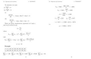
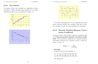
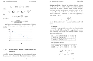
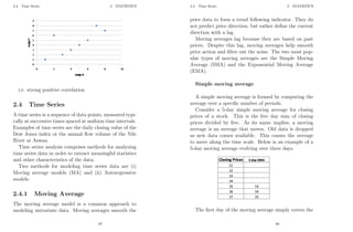
90. 2.3 Regression and Correlation 2 STATISTICS
2.3 Regression and Correlation
2.3.1 Linear regression
We are often interested in looking at the relationship be-
tween two variables (bivariate data). If we can model
this relationship then we can use our model to make pre-
dictions.
A sensible first step would be to plot the data on a
scatter diagram, i.e. pairs of values (xi, yi)
Now we can try to fit a straight line through the data.
We would like to fit the straight line so as to minimise
the sum of the squared distances of the points from the
line. The different between the data value and the fitted
line is called the residual or error and the technique of
often referred to as the method of least squares.
59
2.3 Regression and Correlation 2 STATISTICS
If the equation of the line is given by
y = bx + a
then the error in y, i..e the residual of the ith
data point
(xi, yi) would be
ri = yi − y
= yi − (bxi + a)
We want to minimise
Pn=∞
n=1 r2
i , i.e.
S.R =
n=∞
X
n=1
r2
i =
n=∞
X
n=1
[yi − (bxi + a)]2
We want to find the b and a that minimise
Pn=∞
n=1 r2
i .
S.R =
X
y2
i − 2yi(bxi + a) + (bxi + a)2
=
X
y2
i − 2byixi − 2ayi + b2
x2
i + 2baxi + a2
or
= n ¯
y2 − 2bn ¯
xy − 2anȳ + b2
n ¯
x2 + 2banx̄ + na2
60

91. 2.3 Regression and Correlation 2 STATISTICS
To minimise, we want
(i) ∂(S.R)
∂b = 0
(ii) ∂(S.R)
∂a = 0
(i)
∂(S.R)
∂b
= −2n ¯
xy + 2bn ¯
x2 + 2anx̄ = 0
(ii)
∂(S.R)
∂a
= −2nȳ + 2bnx̄ + 2an = 0
These are linear simultaneous equations in b and a
and can be solved to get
b =
Sxy
Sxx
where
Sxx =
X
(xi − x̄)2
=
X
(x2
i ) −
P
(xi)2
n
and
Sxy =
X
(xi − x̄)(yi − ȳ) =
X
xiyi −
(
P
xi)(
P
yi)
n
a = ȳ − bx̄
Example
x 5 10 15 20 25 30 35 40
y 98 90 81 66 61 47 39 34
X
xi = 180
X
yi = 516
X
x2
i = 5100
X
y2
i = 37228
X
xiyi = 9585
61
2.3 Regression and Correlation 2 STATISTICS
Sxy = 9585 −
180 × 516
8
= −2025
Sxx = 5100 −
1802
8
= 1050
∴ b =
−2025
1050
= −1.929
x̄ =
180
8
= 22.5 ȳ =
516
8
= 64.5
∴ a = 64.5 − (−1.929 × 22.5) = 107.9
i.e.
y = −1.929x + 107.9
62

92. 2.3 Regression and Correlation 2 STATISTICS
2.3.2 Correlation
A measure of how two variables are dependent is their
correlation. When viewing scatter graphs we can often
determine if their is any correlation by sight, e.g.
63
2.3 Regression and Correlation 2 STATISTICS
It is often advantageous to try to quantify the corre-
lation between between two variables, this can be done
in a number of ways, two such methods are described.
2.3.3 Pearson Product-Moment Corre-
lation Coefficient
A measure often used within statistics to quantify this
is the Pearson product-moment correlation coeffi-
cient. This correlation coefficient is a measure of linear
dependence between two variables, giving a value be-
tween +1 and −1.
PMCC r =
Sxy
p
SxxSyy
Example
Consider the previous example, i.e.
x 5 10 15 20 25 30 35 40
y 98 90 81 66 61 47 39 34
We calculated,
64

93. 2.3 Regression and Correlation 2 STATISTICS
Sxy = −2025 and Sxx = 1050
also,
Syy =
X
(yi − ȳ)2
=
X
(y2
i ) −
P
(yi)2
n
i.e
Syy = 37228 −
5162
8
= 3946
therefore,
r =
−2025
√
1050 × 3946
= −0.995
This shows a strong negative correlation and if we were
to plot this using a scatter diagram, we can see this vi-
sually.
2.3.4 Spearman’s Rank Correlation Co-
efficient
Another method of measuring the relationship between
two variables is to use the Spearman’s rank corre-
65
2.3 Regression and Correlation 2 STATISTICS
lation coeffieint. Instead of dealing with the values
of the variables as in the product moment correlation
coefficient, we assign a number (rank) to each variable.
We then calculate a correlation coefficient based on the
ranks. The calculated value is called the Spearmans
Rank Correlation Coefficient, rs, and is an approxima-
tion to the PMCC.
rs = 1 −
6
P
d2
i
n(n2 − 1)
where d is the difference in ranks and n is the number of
pairs.
Example
Consider two judges who score a dancing championship
and are tasked with ranking the competitors in order.
The following table shows the ranking that the judges
gave the competitors.
Competitor A B C D E F G H
JudgeX 3 1 6 7 5 4 8 2
JudgeY 2 1 5 8 4 3 7 6
calculating d2
, we get
difference d 1 0 1 1 1 1 1 4
difference2
d2
1 0 1 1 1 1 1 16
∴
X
d2
i = 22 and n = 8
rs = 1 −
6 × 22
8(82 − 1)
= 0.738
66

94. 2.4 Time Series 2 STATISTICS
i.e. strong positive correlation
2.4 Time Series
A time series is a sequence of data points, measured typi-
cally at successive times spaced at uniform time intervals.
Examples of time series are the daily closing value of the
Dow Jones index or the annual flow volume of the Nile
River at Aswan.
Time series analysis comprises methods for analyzing
time series data in order to extract meaningful statistics
and other characteristics of the data.
Two methods for modeling time series data are (i)
Moving average models (MA) and (ii) Autoregressive
models.
2.4.1 Moving Average
The moving average model is a common approach to
modeling univariate data. Moving averages smooth the
67
2.4 Time Series 2 STATISTICS
price data to form a trend following indicator. They do
not predict price direction, but rather define the current
direction with a lag.
Moving averages lag because they are based on past
prices. Despite this lag, moving averages help smooth
price action and filter out the noise. The two most pop-
ular types of moving averages are the Simple Moving
Average (SMA) and the Exponential Moving Average
(EMA).
Simple moving average
A simple moving average is formed by computing the
average over a specific number of periods.
Consider a 5-day simple moving average for closing
prices of a stock. This is the five day sum of closing
prices divided by five. As its name implies, a moving
average is an average that moves. Old data is dropped
as new data comes available. This causes the average
to move along the time scale. Below is an example of a
5-day moving average evolving over three days.
The first day of the moving average simply covers the
68

95. 2.4 Time Series 2 STATISTICS
last five days. The second day of the moving average
drops the first data point (11) and adds the new data
point (16). The third day of the moving average contin-
ues by dropping the first data point (12) and adding the
new data point (17). In the example above, prices grad-
ually increase from 11 to 17 over a total of seven days.
Notice that the moving average also rises from 13 to 15
over a three day calculation period. Also notice that
each moving average value is just below the last price.
For example, the moving average for day one equals 13
and the last price is 15. Prices the prior four days were
lower and this causes the moving average to lag.
Exponential moving average
Exponential moving averages reduce the lag by apply-
ing more weight to recent prices. The weighting applied
to the most recent price depends on the number of pe-
riods in the moving average. There are three steps to
calculating an exponential moving average. First, calcu-
late the simple moving average. An exponential moving
average (EMA) has to start somewhere so a simple mov-
ing average is used as the previous period’s EMA in the
first calculation. Second, calculate the weighting multi-
plier. Third, calculate the exponential moving average.
The formula below is for a 10-day E.
Ei+1 = 2−(n+1)
(Pi+1 − Ei) + Ei
69
2.4 Time Series 2 STATISTICS
A 10-period exponential moving average applies an
18.18% weighting to the most recent price. A 10-period
EMA can also be called an 18.18% EMA.
A 20-period EMA applies a 9.52% weighing to the
most recent price 2
20+1 = .0952. Notice that the weight-
ing for the shorter time period is more than the weighting
for the longer time period. In fact, the weighting drops
by half every time the moving average period doubles.
70

96. 2.4 Time Series 2 STATISTICS
2.4.2 Autoregressive models
Autoregressive models are models that describe random
processes (denote here as et) that can be described by
a weighted sum of its previous values and a white noise
error.
An AR(1) process is a first-order one process, meaning
that only the immediately previous value has a direct
effect on the current value
et = ret−1 + ut
where r is a constant that has absolute value less than
one, and ut is a white noise process drawn from a distri-
71
2.4 Time Series 2 STATISTICS
bution with mean zero and finite variance, often a normal
distribution.
An AR(2) would have the form
et = r1et−1 + r2et−2 + ut
and so on. In theory a process might be represented
by an AR(∞).
72

97. Mathematical Preliminaries
Introduction to Probability
Preliminaries
Randomness lies at the heart of …nance and whether terms uncertainty or risk are used, they refer to the
random nature of the …nancial markets. Probability theory provides the necessary structure to model the
uncertainty that is central to …nance. We begin by de…ning some basic mathematical tools.
The set of all possible outcomes of some given experiment is called the sample space. A particular
outcome ! 2 is called a sample point.
An event is a set of outcomes, i.e. .
To a set of basic outcomes !i we assign real numbers called probabilities, written P (!i) = pi: Then for
any event E;
P (E) =
X
!i2E
pi
Example 1
Experiment: A dice is rolled and the number appearing on top is observed. The sample space consists
of the 6 possible numbers:
= f1; 2; 3; 4; 5; 6g
If the number 4 appears then ! = 4 is a sample point, clearly 4 2 .
Let 1, 2, 3 = events that an even, odd, prime number occurs respectively.
So
1 = f2; 4; 6g ; 2 = f1; 3; 5g ; 3 = f2; 3; 5g
1 [ 3 = f 2; 3; 4; 5; 6g event that an even or prime number occurs.
2 3 = f3; 5g event that odd and prime number occurs.
c
3 = f1; 4; 6g event that prime number does not occur (complement of event).
Example 2
Toss a coin twice and observe the sequence of heads (H) and tails (T) that appears. Sample space
= fHH, TT, HT, THg
Let 1 be event that at least one head appears, and 2 be event that both tosses are the same:
1 = fHH, HT, THg , 2 = fHH, TTg
1 2 = fHHg
Events are subsets of , but not all subsets of are events.
1
The basic properties of probabilities are
1. 0 pi 1
2. P ( ) =
X
i
pi = 1 (the sum of the probabilities is always 1).
Random Variables
Outcomes of experiments are not always numbers, e.g. 2 heads appearing; picking an ace from a deck
of cards. We need some way of assigning real numbers to each random event. Random variables assign
numbers to events.
Thus a random variable (RV) X is a function which maps from the sample space to the set of real
numbers
X : ! 2 ! R;
i.e. it associates a number X (!) with each outcome !:
Consider the example of tossing a coin and suppose we are paid £ 1 for each head and we lose £ 1 each time
a tail appears. We know that P (H) = P (T) =
1
2
: So now we can assign the following outcomes
P (1) =
1
2
P ( 1) =
1
2
Mathematically, if our random variable is X; then
X =
+1 if H
1 if T
or using the notation above X : ! 2 fH,Tg ! f 1; 1g :
The probability that the RV takes on each possible value is called the probability distribution.
If X is a RV then
P (X = a) = P (f! 2 : X (!) = ag)
is the probability that a occurs (or X maps onto a).
P (a X b) = probability that X lies in the interval [a; b] =
P (f! 2 : a X (!) bg)
X :
Domain
! R
Range (…nite)
X ( ) = fx1; ::::; xng = fxig1 i n
P [xi] = P [X = xi] = f (xi) 8 i:
So the earlier coin tossing example gives
P (X = 1) =
1
2
; P (X = 1) =
1
2
2

98. f (xi) is the probability distribution of X:
This is called a discrete probability distribution.
xi x1 x2 :::::::::::: xn
f (xi) f (x1) f (x2) :::::::::::: f (xn)
There are two properties of the distribution f (xi)
(i) f (xi) 0 8 i 2 [1; n]
(ii)
n
P
i=1
f (xi) = 1; i.e. sum of all probabilities is one.
Mean/Expectation
The mean measures the centre (average) of the distribution
= E [X] =
n
P
i=1
xi f (xi)
= x1f (x1) + x2f (x2) + ::::: + xnf (xn)
which is equal to the weighted average of all possible values of X together with associated probabilities.
This is also called the …rst moment.
Example:
xi 2 3 8
f (xi) 1
4
1
2
1
4
= E [X] =
3
P
i=1
xif (xi) = 2
1
4
+ 3
1
2
+ 8
1
4
= 4
Variance/Standard Deviation
This measures the spread (dispersion) of X about the mean.
Variance V [X] =
E (X )2
= E X2 2
=
n
P
i=1
x2
i f (xi) 2
= 2
E (X )2
is also called the second moment about the mean.
From the previous example we have = 4; therefore
V [X] = 22 1
4
+ 32 1
2
+ 82 1
4
16
= 5:5 = 2
! = 2:34
Rules for Manipulating Expectations
Suppose X; Y are random variables and ; ; 2 R are constant scalar quantities. Then
3
E [ X] = E [X]
E [X + Y ] = E [X] + E [Y ] ; (linearity)
V [ X + ] = 2
V [X]
E [XY ] = E [X] E [Y ] ;
V [X + Y ] = V [X] + V [Y ]
The last two are provided X; Y are independent.
4

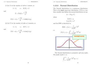
99. Continuous Random Variables
As the number of discrete events becomes very large, individual probabilities f (xi) ! 0: Now look at the
continuous case.
Instead of f (xi) we now have p (x) which is a continuous distribution called as probability density function,
PDF.
P (a X b) =
Z b
a
p (x) dx
The cumulative distribution function F (x) of a RV X is
F (x) = P (X x) =
Z x
1
p (x) dx
F (x) is related to the PDF by
p (x) =
dF
dx
(fundamental theorem of calculus) provided F (x) is di¤erentiable. However unlike F (x) ; p (x) may
have singularities (and may be unbounded).
Special Expectations:
Given any PDF p (x) of X:
Mean = E [X] =
Z
R
xp (x) dx:
Variance 2
= V [X] = E (X )2
=
Z
R
x2
p (x) dx 2
(2nd
moment about the mean).
The nth
moment about zero is de…ned as
n = E [Xn
]
=
Z
R
xn
p (x) dx:
In general, for any function h
E [h (X)] =
Z
R
h (x) p (x) dx:
where X is a RV following the distribution given by p (x) :
Moments about the mean are given by
E [(X )n
] ; n = 2; 3; :::
The special case n = 2 gives the variance 2
:
5
Skewness and Kurtosis
Having looked at the variance as being the second moment about the mean, we now discuss two further
moments centred about ; that provide further important information about the probability distribution.
Skewness is a measure of the asymmetry of a distribution (i.e. lack of symmetry) about its mean. A
distribution that is identical to the left and right about a centre point is symmetric.
The third central moment, i.e. third moment about the mean scaled with 3
. This scaling allows us to
compare with other distributions.
E (X )3
3
is called the skew and is a measure of the skewness (a non-symmetric distribution is called skewed).
Any distribution which is symmetric about the mean has a skew of zero.
Negative values for the skewness indicate data that are skewed left and positive values for the skewness
indicate data that are skewed right.
By skewed left, we mean that the left tail is long relative to the right tail. Similarly, skewed right means
that the right tail is long relative to the left tail.
The fourth centred moment scaled by the square of the variance, called the kurtosis is de…ned
E (X )4
4
:
This is a measure of how much of the distribution is out in the tails at large negative and positive values
of X:
The 4th
central moment is called Kurtosis and is de…ned as
Kurtosis =
E (X )4
4
normal random variable has Kurtosis of 3 irrespective of its mean and standard deviation. Often when
comparing a distribution to the normal distribution, the measure of excess Kurtosis is used, i.e. Kurtosis
of distribution 3.
If a random variable has Kurtosis greater than 3 is called Leptokurtic, if is has Kurtosis less than 3 it
is called platykurtic Leptokurtic is associated with PDF’
s that are simultaneously peaked and have fat tails.
6

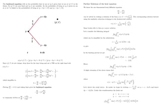
100. Normal Distribution
The normal (or Gaussian) distribution N ( ; 2
) with mean and standard deviation and 2
in turn
is de…ned in terms of its density function
p (x) =
1
p
2
exp
(x )2
2 2
!
:
For the special case = 0 and = 1 it is called the standard normal distribution N (0; 1) :
This is also veri…ed by making the substitution
=
x
in p (x) which gives
( ) =
1
p
2
exp
1
2
2
and clearly has zero mean and unit variance:
E
X
=
1
E [X ] = 0;
V
X
= V
X
Now V [ X + ] = 2
V [X] (standard result), hence
1
2
V [X] =
1
2
: 2
= 1
Its cumulative distribution function is
F (x) =
1
p
2
Z x
1
e
1
2
2
d = P ( 1 X x) :
The skewness of N (0; 1) is zero and its kurtosis is 3:
7
Correlation
The covariance is useful in studying the statistical dependence between two random variables. If X; Y are
RV’
s, then their covariance is de…ned as:
Cov (X; Y ) = E
2
6
4
0
@X E (X)
| {z }
= x
1
A
0
B
@Y E (Y )
| {z }
= y
1
C
A
3
7
5
= E [XY ] x y
which we denote as XY : Note:
Cov (X; X) = E (X x)2
= 2
:
X; Y are correlated if
E (X x) Y y 6= 0:
We can then de…ne an important dimensionless quantity (used in …nance) called the correlation coe¢ cient
and denoted as XY (X; Y ) where
XY =
Cov (X; Y )
x y
:
The correlation can be thought of as a normalised covariance, as j XY j 1; for which the following
conditions are properties:
i. (X; Y ) = (Y; X)
ii. (X; X) = 1
iii. 1 1
XY = 1 ) perfect negative correlation
XY = 1 )perfect correlation
XY = 0 ) X; Y uncorrelated
Why is the correlation coe¢ cient bounded by 1? Justi…cation of this requires a result called the Cauchy-
Schwartz inequality. This is a theorem which most students encounter for the …rst time in linear algebra
(although we have not discussed this). Let’
s start o¤ with the version for random variables (RVs) X and
Y , then the Cauchy-Schwartz inequality is
[E [XY ]]2
E X2
E Y 2
:
We know that the covariance of X; Y is
XY = E [(X X) (Y Y )]
If we put
V [X] = 2
X = E (X X)2
V [Y ] = 2
Y = E (Y Y )2
:
8

101. From Cauchy-Schwartz we have
(E [(X X) (Y Y )])2
E (X X)2
E (Y Y )2
or we can write
2
XY
2
X
2
Y
Divide through by 2
X
2
Y
2
XY
2
X
2
Y
1
and we know that the left hand side above is 2
XY , hence
2
XY =
2
XY
2
X
2
Y
1
and since XY is a real number, this implies j XY j 1 which is the same as
1 XY +1:
Central Limit Theorem
This concept is fundamental to the whole subject of …nance.
Let Xi be any independent identically distributed (i.i.d) random variable with mean and variance 2
;
i.e. X D ( ; 2
) ; where D is some distribution: If we put
Sn =
n
P
i=1
Xi
Then
(Sn n )
p
n
has a distribution that approaches the standard normal distribution as n ! 1:
The distribution of the sum of a large number of independent identically distributed variables will be
approximately normal, regardless of the underlying distribution. That is the beauty of this result.
Conditions:
The Normal distribution is the limiting behaviour if you add many random numbers from any basic-building
block distribution provided the following is satis…ed:
1. Mean of distribution must be …nite and constant
2. Standard deviation of distribution must be …nite and constant
This is a measure of how much of the distribution is out in the tails at large negative and positive values
of X:
9
Moment Generating Function
The moment generating function of X; denoted MX ( ) is given by
MX ( ) = E e X
=
Z
R
e x
p (x) dx
provided the expectation exists. We can expand as a power series to obtain
MX ( ) =
1
X
n=0
n
E (Xn
)
n!
so the nth
moment is the coe¢ cient of n
=n!; or the nth
derivative evaluated at zero.
How do we arrive at this result?
We use the Taylor series expansion for the exponential function:
Z
R
e x
p (x) dx =
Z
R
1 + x +
( x)2
2!
+
( x)3
3!
+ ::::::
!
p (x) dx
=
Z
R
p (x) dx
| {z }
1
+
Z
R
xp (x) dx
| {z }
E(X)
+
2
2!
Z
R
x2
p (x) dx
| {z }
E(X2)
+
3
3!
Z
R
x3
p (x) dx
| {z }
E(X3)
+ ::::
= 1 + E (X) +
2
2!
E X2
+
3
3!
E X3
+ ::::
=
1
X
n=0
n
E (Xn
)
n!
:
10

102. Calculating Moments
The kth
moment mk of the random variable X can now be obtained by di¤erentiating, i.e.
mk = M
(k)
X ( ) ; k = 0; 1; 2; :::
M
(k)
X ( ) =
dk
d k
MX ( )
=0
So what is this result saying? Consider MX ( ) =
1
X
n=0
n
E(Xn)
n!
MX ( ) = 1 + E [X] +
2
2!
E X2
+
3
3!
E X3
+ :::: +
n
n!
E [Xn
]
As an example suppose we wish to obtain the second moment; di¤erentiate twice with respect to
d
d
MX ( ) = E [X] + E X2
+
2
2
E X3
+ :::: +
n 1
(n 1)!
E [Xn
]
and for the second time
d2
d 2 MX ( ) = E X2
+ E X3
+ :::: +
n 2
(n 2)!
E [Xn
] :
Setting = 0; gives
d2
d 2 MX (0) = E X2
which captures the second moment E [X2
]. Remember we will already have an expression for MX ( ) :
A useful result in …nance is the MGF for the normal distribution. If X N ( ; 2
), then we can construct
a standard normal N (0; 1) by setting =
X
=) X = + :
The MGF is
MX ( ) = E e x
= E e ( + )
= e E e
So the MGF of X is therefore equal to the MGF of but with replaced by :This is much nicer than
trying to calculate the MGF of X N ( ; 2
) :
E e =
1
p
2
Z 1
1
e x
e x2=2
dx =
1
p
2
Z 1
1
e x x2=2
dx
=
1
p
2
Z 1
1
e
1
2 (x2 2 x+ 2 2
)dx =
1
p
2
Z 1
1
e
1
2
(x )2
+ 1
2
2
dx
= e
1
2
2 1
p
2
Z 1
1
e
1
2
(x )2
dx
Now do a change of variable - put u = x
E e = e
1
2
2 1
p
2
Z 1
1
e
1
2
u2
du
= e
1
2
2
11
Thus
MX ( ) = e E e
= e + 1
2
2 2
To get the simpler formula for a standard normal distribution put = 0; = 1 to get MX ( ) = e
1
2
2
:
We can now obtain the …rst four moments for a standard normal
m1 =
d
d
e
1
2
2
=0
= e
1
2
2
=0
= 0
m2 =
d2
d 2 e
1
2
2
=0
= 2
+ 1 e
1
2
2
=0
= 1
m3 =
d3
d 3 e
1
2
2
=0
= 3
+ 3 e
1
2
2
=0
= 0
m4 =
d4
d 4 e
1
2
2
=0
= 4
+ 6 2
+ 3 e
1
2
2
=0
= 3
The latter two are particularly useful in calculating the skew and kurtosis.
If X and Y are independent random variables then
MX+Y ( ) = E e (x+y)
= E e x
e y
= E e x
E e y
= MX ( ) MY ( ) :
12

103. Calculus Refresher
Taylor for two Variables
Assuming that a function f (x; t) is di¤erentiable enough, near x = x0; t = t0;
f (x; t) = f (x0; t0) + (x x0) fx (x0; t0) +
(t t0) ft (x0; t0)
+
1
2
2
4
(x x0)2
fxx (x0; t0)
+2 (x x0) (t t0) fxt (x0; t0)
+ (t t0)2
ftt (x0; t0)
3
5 + ::::
That is,
f (x; t) = constant + linear + quadratic
+::::
The error in truncating this series after the second order terms tends to zero faster than the included
terms. This result is particularly important for Itô’
s lemma in Stochastic Calculus.
Suppose a function f = f (x; y) and both x; y change by a small amount, so x ! x+ x and y ! y + y;
then we can examine the change in f using a two dimensional form of Taylor
f (x + x; y + y) = f (x; y) + fx x + fy y +
1
2
fxx x2
+
1
2
fyy y2
+
fxy x y + O x2
; y2
:
By taking f (x; y) to the lhs, writing
df = f (x + x; y + y) f (x; y)
and considering only linear terms, i.e.
df =
@f
@x
x +
@f
@y
y
we obtain a formula for the di¤erential or total change in f:
13
Integration
There are two ways to show the following important result
Z
R
e x2
=
p
:
The …rst can be thought of as the ’
poor man’
s’derivation.
The CDF for the Normal Distribution is
N (x) =
1
p
2
Z x
1
e s2=2
ds
If x ! 1 then we know (by the fact that the area under a PDF has to sum to unity) that
1
p
2
Z 1
1
e s2=2
ds = 1:
Make the substitution x = s=
p
2 to give dx = ds=
p
2; hence the integral becomes
p
2
Z 1
1
e x2
dx =
p
2
and hence we obtain Z 1
1
e x2
dx =
p
From this we also note that
R 1
0
e x2
dx =
p
2
because e x2
is an even function.
The second requires double integration. Put I =
Z
R
e x2
dx so that
I2
=
Z
R
e x2
dx
Z
R
e y2
dy
=
Z
R
Z
R
e (x2+y2
)dxdy
The region of integration is a square centered at the origin of in…nite dimension
x 2 ( 1; 1)
y 2 ( 1; 1)
i.e. the complete 2D plane. Introduce plane polars
x = r cos
y = r sin
dxdy ! rdrd
The region of integration is now a circle centred at the origin of in…nite radius
0 r 1
0 2
so the problem becomes
I2
=
Z 2
0
Z 1
0
e r2
rdrd
=
1
2
Z 2
0
d =
Hence
I =
Z 1
1
e x2
dx =
p
:
14

104. Review of Di¤erential Equations
Cauchy Euler Equation
An equation of the form
Ly = ax2 d2
y
dx2
+ x
dy
dx
+ cy = g (x)
is called a Cauchy-Euler equation.
To solve the homogeneous part, we look for a solution of the form
y = x
So y0
= x 1
! y00
= ( 1) x 2
, which upon substitution yields the quadratic, A.E.
a 2
+ b + c = 0;
where b = ( a) which can be solved in the usual way - there are 3 cases to consider, depending upon
the nature of b2
4ac.
Case 1: b2
4ac 0 ! 1, 2 2 R - 2 real distinct roots
GS y = Ax 1
+ Bx 2
Case 2: b2
4ac = 0 ! = 1 = 2 2 R - 1 real (double fold) root
GS y = x (A + B ln x)
Case 3: b2
4ac 0 ! = i 2 C - pair of complex conjugate roots
GS y = x (A cos ( ln x) + B sin ( ln x))
Example
Consider the following Euler type problem
1
2
2
S2 d2
V
dS2
+ rS
dV
dS
rV = 0;
V (0) = 0; V (S ) = S E
where the constants E; S ; ; r 0. We are given that the roots of A.E m are real with m 0 m+:
Look for a solution of the form General Solution is
V (S) = ASm+
+ BSm
:
V (0) = 0 =) B = 0 else we have division by zero
V (S) = ASm+
15
To …nd A use the second condition V (S ) = S E
V (S ) = A (S )m+
= S E ! A =
S E
(S )m+
hence
V (S) =
S E
(S )m+
(S)m+
= (S E)
S
S
m+
:
Similarity Methods
f (x; y) is homogeneous of degree t 0 if f ( x; y) = t
f (x; y) :
1. f (x; y) =
p
(x2 + y2)
f ( x; y) =
q
( x)2
+ ( y)2
=
p
[(x2 + y2)] = f (x; y)
g (x; y) = x+y
x y
then
g ( x; y) = x+ y
x y
= 0 x+y
x y
= 0
g (x; y)
2. h (x; y) = x2
+ y3
h ( x; y) = ( x)2
+ ( y)3
= 2
x2
+ 3
y3
6= t
x2
+ y3
for any t. So h is not homogeneous.
Consider the function
F (x; y) = x2
x2+y2
If for any 0 we write
x0
= x; y0
= y
then
dy0
dx0
=
dy
dx
; x2
x2+y2 = x02
x02
+y02 :
We see that the equation is invariant under the change of variables. It also makes sense to look for a
solution which is also invariant under the transformation. One choice is to write
v =
y
x
=
y0
x0
so write
y = vx:
De…nition The di¤erential equation
dy
dx
= f (x; y) is said to be homogeneous when f (x; y) is homogeneous
of degree t for some t:
Method of Solution
Put y = vx where v is some (as yet) unknown function. Hence we have
dy
dx
=
d
dx
(vx) = x
dv
dx
+ v
dx
dx
= v0
x + v
16

105. Hence
f (x; y) = f (x; vx)
Now f is homogeneous of degree t so
f (x; vx) = xt
f (1; v)
The di¤erential equation now becomes
v0
x + v = xt
f (1; v)
which is not always solvable - the method may not work. But when t = 0 (homogeneous of degree zero)
then xt
= 1: Hence
v0
x + v = f (1; v)
or
x
dv
dx
= f (1; v) v
which is separable, i.e. Z
dv
f (1; v) v
=
Z
dx
x
+ c
and the method is guaranteed to work.
Example
dy
dx
=
y x
y + x
First we check:
y x
y + x
= 0 y x
y + x
which is homogeneous of degree zero. So put y = vx
v0
x + v = f (x; yx) =
vx x
vx + x
=
v 1
v + 1
= f (1; v)
therefore
v0
x =
v 1
v + 1
v
=
(1 + v2
)
v + 1
and the D.E is now separable
Z
v + 1
v2 + 1
dv =
Z
1
x
dx
Z
v
v2 + 1
dv +
Z
1
v2 + 1
dv =
Z
1
x
dx
1
2
ln 1 + v2
+ arctan v = ln x + c
1
2
ln x2
1 + v2
+ arctan v = c
Now we turn to the original problem, so put v =
y
x
1
2
ln x2
1 +
y2
x2
+ arctan
y
x
= c
which simpli…es to
1
2
ln x2
+ y2
+ arctan
y
x
= c:
17
The Error Function
We begin by solving the following initial value problem (IVP)
dy
dx
2xy = 2; y (0) = 1:
which is clearly a linear equation. The integrating factor is R (x) = exp ( x2
) which multiplying through
gives
e x2 dy
dx
2xy = 2e x2
d
dx
e x2
y = 2e x2
Z x
0
d e t2
y = 2
Z x
0
e t2
dt
Concentrate on the lhs and noting the IC y (0) = 1
e t2
y
x
0
= e x2
y (x) y (0) = e x2
y (x) 1
hence
e x2
y (x) 1 = 2
Z x
0
e t2
dt
y (x) = ex2
1 + 2
Z x
0
e t2
dt
We cannot simplify the integral on the rhs any further if we wish this to remain as a closed form solution.
However we note the following non-elementary integrals
erf (x) =
2
p
Z x
0
e s2
ds;
erf c (x) =
2
p
Z 1
x
e s2
ds:
This is the error function and complimentary error function, in turn.
The solution to the IVP can now be written
y (x) = ex2
1 +
p
erf (x)
So, for example
Z x1
x0
e x2
dx =
Z x1
0
e x2
dx
Z x0
0
e x2
dx
=
p
2
(erf (x1) erf (x0)) :
Working: We are using erf (x) =
2
p
R x
0
e s2
ds which rearranges to give
Z x
0
e s2
ds =
p
2
erf (x)
18

106. then
Z x1
x0
Z 0
x0
+
Z x1
0
=
Z x0
0
+
Z x1
0
=
Z x1
0
e x2
dx
Z x0
0
e x2
dx
=
p
2
(erf (x1) erf (x0))
19
The Dirac delta function
The delta function denoted (x) ; is a very useful ’
object’in applied maths and more recently in quant
…nance. It is the mathematical representation of a point source e.g. force, payment. Although labelled
a function, it is more of a distribution or generalised function. Consider the following de…nition for a
piecewise function
f (x) =
1
;
0;
x 2 2
; 2
otherwise
Now put the delta function equal to the above for the following limiting value
(x) = lim
!0
f (x)
What is happening here? As decreases we note the ’
hat’ narrows whilst becoming taller eventually
becoming a spike. Due to the de…nition, the area under the curve (i.e. rectangle) is …xed at 1, i.e. 1
;
which is independent of the value of : So mathematically we can write in integral terms
Z 1
1
f (x) dx =
Z
2
1
f (x) dx +
Z
2
2
f (x) dx +
Z 1
2
f (x) dx
=
1
= 1 for all :
Looking at what happens in the limit ! 0; the spike like (singular) behaviour at the origin gives the
following de…nition
(x) =
1 x = 0
0 x 6= 0
with the property Z 1
1
(x) dx = 1:
There are many ways to de…ne (x) : Consider the Gaussian/Normal distribution with pdf
G (x) =
1
p
2
exp
x2
2 2
:
The function takes its highest value at x = 0; as jxj ! 1 there is exponential decay away from the origin.
If we stay at the origin, then as decreases, G (x) exhibits the earlier spike (as it shoots up to in…nity),
so
lim
!0
G (x) = (x) :
20

107. The normalising constant 1
p
2
ensures that the area under the curve will always be unity.
The graph below shows G (x) for values = 2:0 (royal blue); 1:0 (red); 0:5 (green); 0:25 (purple); 0:125 (turquoise);
the Gaussian curve becomes slimmer and more peaked as decreases.
G (x) is plotted for = 0:01
21
Now generalise this de…nition by centring the function f (x) at any point x0
: So
(x x0
) = lim
!0
f (x x0
)
Z 1
1
(x x0
) dx = 1:
The …gure will be as before, except that now centered at x0
and not at the origin as before. So we see two
de…nitions of (x) : Another is the Cauchy distribution
L (x) =
1
x2 + 2
So here
(x) = lim
!0
1
x2 + 2
Now suppose we have a smooth function g (x) and consider the following integral problem
Z 1
1
g (x) (x x0) dx = g (x0)
This sifting property of the delta function is a very important one.
Heaviside Function
The Heaviside function, denoted by H (), is a discontinuous function whose value is zero for negative
parameters and one for positive arguments
H (x) =
1 x 0
0 x 0
Some de…nitions have
H (x) =
8
:
1 x 0
1
2
x = 0
0 x 0
22

108. and
H (x) =
1 x 0
0 x 0
It is an example of the general class of step functions.
23
Probability Distributions
At the heart of modern …nance theory lies the uncertain movement of …nancial quantities. For modelling
purposes we are concerned with the evolution of random events through time.
A di¤usion process is one that is continuous in space, while a random walk is a process that is discrete.
The random path followed by the process is called a realization. Hence when referring to the path traced
out by a …nancial variable will be termed as an asset price realization.
The mathematics can be achieved by the concept of a transition density function and is the connection
between probability theory and di¤erential equations.
Trinomial Random Walk
A trinomial random walk models the dynamics of a random variable, with value y at time t: is a
probability. y is the size of the move in y.
The Transition Probability Density Function
The transition pdf is denoted by
p (y; t; y0
; t0
)
We can gain information such as the centre of the distribution, where the random variable might be in the
long run, etc. by studying its probabilistic properties. So the density of particles di¤using from (y; t) to
(y0
; t0
) :
Think of (y; t) as current (or backward) variables and (y0
; t0
) as future ones.
The more basic assistance it gives is with
P (a y0
b at t0
j y at t) =
Z b
a
p (y; t; y0
; t0
) dy0
i.e. the probability that the random variable y0
lies in the interval a and b;at a future time t0
; given it
started out at time t with value y:
24

109. p (y; t; y0
; t0
) satis…es two equations:
Forward equation involving derivatives with respect to the future state (y0
; t0
) : Here (y; t) is a starting
point and is ’
…xed’
.
Backward equation involving derivatives with respect to the current state (y; t) : Here (y0
; t0
) is a future
point and is ’
…xed’
. The backward equation tells us the probability that we were at (y; t) given that we
are now at (y0
; t0
) ; which is …xed.
The mathematics: Start out at a point (y; t) : We want to answer the question, what is the probability
density function of the position y0
of the di¤usion at a later time t0
?
This is known as the transition density function written p (y; t; y0
; t0
) and represents the density of
particles di¤using from (y; t) to (y0
; t0
) : How can we …nd p?
Forward Equation
Starting with a trinomial random walk which is discrete we can obtain a continuous time process to obtain
a partial di¤erential equation for the transition probability density function (i.e. a time dependent PDF).
So the random variable can either rise or fall with equal probability 1
2
and remain at the same location
with probability 1 2 :
Suppose we are at (y0
; t0
) ; how did we get there?
At the previous step time step we must have been at one of (y0
+ y; t0
t) or (y0
y; t0
t) or
(y0
; t0
t) :
So
p (y; t; y0
; t0
) = p (y; t; y0
+ y; t0
t) + (1 2 ) p (y; t; y0
; t0
t)
+ p (y; t; y0
y; t0
t)
25
Taylor series expansion gives (omit the dependence on (y; t) in your working as they will not change)
p (y0
+ y; t0
t) = p (y0
; t0
)
@p
@t0
t +
@p
@y0
y + 1
2
@2
p
@y02 y2
+ :::
p (y0
; t0
t) = p (y0
; t0
)
@p
@t0
t + :::
p (y0
y; t0
t) = p (y0
; t0
)
@p
@t0
t
@p
@y0
y + 1
2
@2
p
@y02 y2
+ :::
Substituting into the above
p (y0
; t0
) = p (y0
; t0
)
@p
@t0
t +
@p
@y0
y + 1
2
@2
p
@y02 y2
+
(1 2 ) p (y0
; t0
)
@p
@t0
t+
+ p (y0
; t0
)
@p
@t0
t
@p
@y0
y + 1
2
@2
p
@y02 y2
0 =
@p
@t0
t +
@2
p
@y02 y2
@p
@t0
=
y2
t
@2
p
@y02
Now take limits. This only makes sense if y2
t
is O (1) ; i.e. y2
O ( t) and letting y; t ! 0 gives
the equation
@p
@t0
= c2 @2
p
@y02 ;
where c2
= y2
t
: This is called the forward Kolmogorov equation. Also called Fokker Planck equation.
It shows how the probability density of future states evolves, starting from (y; t) :
26

110. The Backward Equation
The backward equation is particularly important in the context of …nance, but also a source of much
confusion. Illustrate with the ’
real life’example that Wilmott uses.
Wilmott uses a Trinomial Random Walk
So 3 possible states at the next time step. Here 1=2:
27
At 7pm you are at the o¢ ce - this is the point (y; t)
At 8pm you will be at one of three places:
x The Pub - the point (y + y; t + t) ;
x Still at the o¢ ce - the point (y; t + t) ;
x Madame Jojo’
s - the point (y y; t + t)
We are interested in the probability of being tucked up in bed at midnight (y0
; t0
) ; given that we were at
the o¢ ce at 7pm:
Looking at the earlier …gure, we can only get to bed at midnight via either
the pub
the o¢ ce
Madame Jojo’
s
at 8pm.
What happens after 8pm doesn’
t matter - we don’
t care, you may not even remember! We are only
concerned with being in bed at midnight.
The earlier …gure shows many di¤erent paths, only the ones ending up in ’
our’bed are of interest to us.
In words: The probability of going from the o¢ ce at 7pm to bed at midnight is
the probability of going to the pub from the o¢ ce and then to bed at midnight plus
the probability of staying in the o¢ ce and then going to bed at midnight plus
the probability of going to Madame Jojo’
s from the o¢ ce and then to bed at midnight
The above can be expressed mathematically as
p (y; t; y0
; t0
) = p (y + y; t + t; y0
; t0
) + (1 2 ) p (y; t + t; y0
; t0
) +
p (y y; t + t; y0
; t0
) :
Performing a Taylor expansion gives dropping y0
; t0
p (y; t) = p +
@p
@t
t +
@p
@y
y +
1
2
@2
p
@y2
y2
+ ::
+ (1 2 ) p
@p
@t
t + ::
p +
@p
@t
t
@p
@y
y +
1
2
@2
p
@y2
y2
+ :: :
Most of the terms cancel and leave
0 = t
@p
@t
+ y2 @2
p
@y2
+ :::
28

111. which becomes
0 =
@p
@t
+
y2
t
@2
p
@y2
+ :::
and letting y2
t
= c2
where c is non-zero and …nite as t; y ! 0; we have
@p
@t
+ c2 @2
p
@y2
= 0
Solving the Forward Equation
The equation is
@p
@t0
= c2 @2
p
@y02
for the unknown function p = p (y0
; t0
) : The idea is to obtain a solution in terms of Gaussian curves. Let’
s
drop the primed notation.
We assume a solution of the following form exists:
p (y; t) = ta
f
y
tb
where a; b are constants to be determined. So put
=
y
tb
= yt b
;
which is a dimensionless variable. We have the following derivatives
@
@y
= t b
;
@
@t
= byt b 1
we can now say
p (y; t) = ta
f ( )
therefore
@p
@y
=
@p
@
@
@y
= ta
f0
( ) :t b
= ta b
f0
( )
@2
p
@y2
=
@
@y
@p
@y
=
@
@y
ta b
f0
( )
=
@
@y
@
@
ta b
f0
( )
= ta b 1
tb
@
@
f0
( ) = ta 2b
f00
( )
@p
@t
= ta @
@t
f ( ) + ata 1
f ( )
we can use the chain rule to write
@
@t
f ( ) =
@f
@
:
@
@t
= byt b 1
f0
( )
so we have
@p
@t
= ata 1
f ( ) byta b 1
f0
( )
29
and then substituting these expressions in to the pde gives
ata 1
f ( ) byta b 1
f0
( ) = c2
ta 2b
f00
:
We know from that
y = tb
hence the equation above becomes
ata 1
f ( ) b ta 1
f0
( ) = c2
ta 2b
f00
:
For the similarity solution to exist we require the equation to be independent of t; i.e. a 1 = a 2b =)
b = 1=2; therefore
af
1
2
f0
= c2
f00
thus we have so far
p = ta
f y
p
t
which gives us a whole family of solutions dependent upon the choice of a:
We know that p represents a pdf, hence
Z
R
p (y; t) dy = 1 =
Z
R
ta
f y
p
t
dy
change of variables u = y=
p
t ! du = dy=
p
t so the integral becomes
ta+1=2
Z 1
1
f (u) du = 1
which we need to normalize independent of time t: This is only possible if a = 1=2:
So the D.E becomes
1
2
(f + f0
) = c2
f00
:
We have an exact derivative on the lhs, i.e.
d
d
( f) = f + f0
, hence
1
2
d
d
( f) = c2
f00
and we can integrate once to get
1
2
( f) = c2
f0
+ K:
We obtain K from the following information about a probability density, as ! 1
f ( ) ! 0
f0
( ) ! 0
hence K = 0 in order to get the correct solution, i.e.
1
2
( f) = c2
f0
which can be solved as a simple …rst order variable separable equation:
f ( ) = A exp 1
4c2
2
:
30

112. A is a normalizing constant, so write
A
Z
R
exp 1
4c2
2
d = 1:
Now substitute x = =2c; so 2cdx = d
2cA
Z
R
exp x2
dx
| {z }
=
p
= 1;
which gives A = 1=2c
p
: Returning to
p (y; t) = t 1=2
f ( )
becomes
p (y0
; t0
) =
1
2c
p
t0
exp
y02
4t0c2
!
:
This is a pdf for a variable y that is normally distributed with mean zero and standard deviation c
p
2t;
which we ascertained by the following comparison:
1
2
y02
2t0c2
:
1
2
(x )2
2
i.e. 0 and 2
2t0
c2
:
This solution is also called the Source Solution or Fundamental Solution.
If the random variable y0
has value y at time t then we can generalize to
p (y; t; y0
; t0
) =
1
2c
p
(t0 t)
exp
(y0
y)2
4c2 (t0 t)
!
31
At t0
= t this is now a Dirac delta function (y0
y) : This particle is known to start from (y; t) and
di¤uses out to (y0
; t0
) with mean y and variance (t0
t)
Recall this behaviour of decay away from one point y, unbounded growth at that point and constant area
means that p (y; t; y0
; t0
) has turned in to a Dirac delta function (y0
y) as t0
! t.
32

113. Using a Binomial random walk
The earlier results can also be obtained using a symmetric random walk. Consider the following (two step)
binomial random walk. So the random variable can either rise or fall with equal probability.
y is the random variable and t is a time step. y is the size of the move in y:
P [ y] = P [ y] = 1=2:
Suppose we are at (y0
; t0
) ; how did we get there? At the previous step time step we must have been at one
of (y0
+ y; t0
t) or (y0
y; t0
t) :
So
p (y0
; t0
) = 1
2
p (y0
+ y; t0
t) + 1
2
p (y0
y; t0
t)
Taylor series expansion gives
p (y0
+ y; t0
t) = p (y0
; t0
)
@p
@t0
t +
@p
@y0
y + 1
2
@2
p
@y02 y2
+ :::
p (y0
y; t0
t) = p (y0
; t0
)
@p
@t0
t
@p
@y0
y + 1
2
@2
p
@y02 y2
+ :::
Substituting into the above
p (y0
; t0
) = 1
2
p (y0
; t0
)
@p
@t0
t +
@p
@y0
y + 1
2
@2
p
@y02 y2
+1
2
p (y0
; t0
)
@p
@t0
t
@p
@y0
y + 1
2
@2
p
@y02 y2
33
0 =
@p
@t0
t + 1
2
@2
p
@y02 y2
@p
@t0
= 1
2
y2
t
@2
p
@y02
Now take limits. This only makes sense if y2
t
is O (1) ; i.e. y2
O ( t) and letting y; t ! 0 gives the
equation
@p
@t0
= 1
2
@2
p
@y02
This is called the forward Kolmogorov equation. Also called Fokker Planck equation.
It shows how the probability density of future states evolves, starting from (y; t) :
A particular solution of this is
p (y; t; y0
; t0
) =
1
p
2 (t0 t)
exp
(y0
y)2
2 (t0 t)
!
At t0
= t this is equal to (y0
y). The particle is known to start from (y; t) and its density is normal
with mean y and variance t0
t:
34

114. The backward equation tells us the probability that we are at (y; t) given that we are at (y0
; t0
) in the
future: So (y0
; t0
) are now …xed and (y; t) are variables. So the probability of being at (y; t) given we are
at y0
at t0
is linked to the probabilities of being at (y + y; t + t) and (y y; t + t) :
p (y; t; y0
; t0
) = 1
2
p (y + y; t + t; y0
; t0
) + 1
2
p (y y; t + t; y0
; t0
)
Since (y0
; t0
) do not change, drop these for the time being and use a TSE on the right hand side
p (y; t) =
1
2
p (y; t) +
@p
@t
t +
@p
@y
y + 1
2
@2
p
@y2 y2
+ ::: +
1
2
p (y; t) +
@p
@t
t
@p
@y
y + 1
2
@2
p
@y2 y2
+ :::
which simpli…es to
0 =
@p
@t
+ 1
2
y2
t
@2
p
@y2 :
Putting y2
t
= O (1) and taking limit gives the backward equation
@p
@t
= 1
2
c2 @2
p
@y2 :
or commonly written as
@p
@t
+
1
2
@2
p
@y2 = 0
35
Further Solutions of the heat equation
We know the one dimensional heat/di¤usion equation
@u
@t
=
@2
u
@x2
can be solved by seeking a solution of the form u (x; t) = t
x
t
: The corresponding solution derived
using the similarity reduction technique is the fundamental solution
u (x; t) =
1
2
p
t
exp
x2
4t
:
Some books refer to this as a source solution.
Let’
s consider the following integral
lim
t !0
Z 1
1
u (y; t) f (y) dy
which can be simpli…ed by the substitution
s =
y
2
p
t
=) 2
p
tds = dy
to give
lim
t !0
1
2
p
t
Z 1
1
exp s2
f 2
p
ts 2
p
tds:
In the limiting process we get
f (0)
1
p
Z 1
1
exp s2
ds = f (0)
1
p
p
= f (0) :
Hence
lim
t !0
Z 1
1
u (y; t) f (y) dy = f (0) :
A slight extension of the above shows that
lim
t !0
Z 1
1
u (x y; t) f (y) dy = f (x) ;
where
u (x y; t) =
1
2
p
t
exp
(x y)2
4t
!
:
Let’
s derive the result above. As earlier we begin by writing s =
x y
2
p
t
=) y = x 2
p
ts and hence
dy = 2
p
tds: Under this transformation the limits are
y = 1 ! s = 1
y = 1 ! s = 1
1
2
p
t
Z 1
1
exp s2
f x 2
p
ts 2
p
tds ds
36

115. lim
t !0
1
p
Z 1
1
exp s2
f x 2
p
ts ds
= f (x) 1
p
Z 1
1
exp s2
ds
= f (x) 1
p
p
and
lim
t !0
Z 1
1
u (x y; t) f (y) dy = f (x) :
Since the heat equation is a constant coe¢ cient PDE, if u (x; t) satis…es it, then u (x y; t) is also a solution
for any y:
Recall what it means for an equation to be linear:
Since the heat equation is linear,
1. if u (x y; t) is a solution, so is a multiple f (y) u (x y; t)
2. we can add up solutions. Since f (y) u (x y; t) is a solution for any y; so too is the integral
Z 1
1
u (x y; t) f (y) dy:
Recall, adding can be done in terms of an integral. So we we can summarize by specifying the
following initial value problem
@u
@t
=
@2
u
@x2
u (x; 0) = f (x)
which has a solution
u (x; t) = 1
2
p
t
Z 1
1
exp
(x y)2
4t
!
f (y) dy:
This satis…es the initial condition at t = 0 because we have shown that at that point the value of
this integral is f (x) : Putting t 0 gives a non-existent solution, i.e. the integrand will blow up.
Example 1 Consider the IVP
@u
@t
=
@2
u
@x2
u (x; 0) =
0 if x 0
1 if x 0
We can write down the solution as
u (x; t) = 1
2
p
t
Z 1
1
exp
(x y)2
4t
!
u (y; 0)
| {z }
=f(y)
dy
= 1
2
p
t
Z 0
1
exp
(x y)2
4t
!
:1dy
37
put
s =
y x
p
2t
Z 0
1
becomes
Z x
p
2t
1
1
2
p
t
Z x
2
p
t
1
exp s2
=2
p
2tds
= 1
p
2
Z x
p
2t
1
exp s2
=2 ds
= N x
p
2t
So we have expressed the solution in terms of the CDF.
This can also be solved by using the substitution
b
s =
(y x)
2
p
t
! dy = 2
p
tdb
s
Z 0
1
becomes
Z x
2
p
t
1
1
2
p
t
Z x
2
p
t
1
exp b
s2
2
p
tdb
s
= 1
2
: 2
p
Z 1
x
2
p
t
exp b
s2
db
s
= 1
2
erf c x
2
p
t
so now we have a solution in terms of the complimentary error function.
38

116. Mathematical Preliminaries
Introduction to Probability - Moment Generating Function
The moment generating function of X; denoted MX ( ) is given by
MX ( ) = E e x
=
Z
R
e x
p (x) dx
provided the expectation exists. We can expand as a power series to obtain
MX ( ) =
1
X
n=0
n
E (Xn
)
n!
so the nth
moment is the coe¢ cient of n
=n!; or the nth
derivative evaluated at zero.
How do we arrive at this result?
We use the Taylor series expansion for the exponential function:
Z
R
e x
p (x) dx =
Z
R
1 + x +
( x)2
2!
+
( x)3
3!
+ ::::::
!
p (x) dx
=
Z
R
p (x) dx
| {z }
1
+
Z
R
xp (x) dx
| {z }
E(X)
+
2
2!
Z
R
x2
p (x) dx
| {z }
E(X2)
+
3
3!
Z
R
x3
p (x) dx
| {z }
E(X3)
+ ::::
= 1 + E (X) +
2
2!
E X2
+
3
3!
E X3
+ ::::
=
1
X
n=0
n
E (Xn
)
n!
:
1
Calculating Moments
The kth
moment mk of the random variable X can now be obtained by di¤erentiating, i.e.
mk = M
(k)
X ( ) ; k = 0; 1; 2; :::
M
(k)
X ( ) =
dk
d k
MX ( )
=0
So what is this result saying? Consider MX ( ) =
1
X
n=0
n
E(Xn)
n!
MX ( ) = 1 + E [X] +
2
2!
E X2
+
3
3!
E X3
+ :::: +
n
n!
E [Xn
]
As an example suppose we wish to obtain the second moment; di¤erentiate twice with respect to
d
d
MX ( ) = E [X] + E X2
+
2
2
E X3
+ :::: +
n 1
(n 1)!
E [Xn
]
and for the second time
d2
d 2 MX ( ) = E X2
+ E X3
+ :::: +
n 2
(n 2)!
E [Xn
] :
Setting = 0; gives
d2
d 2 MX (0) = E X2
which captures the second moment E [X2
]. Remember we will already have an expression for MX ( ) :
A useful result in …nance is the MGF for the normal distribution. If X N ( ; 2
), then we can construct
a standard normal N (0; 1) by setting =
X
=) X = + :
The MGF is
MX ( ) = E e x
= E e ( + )
= e E e
So the MGF of X is therefore equal to the MGF of but with replaced by :This is much nicer than
trying to calculate the MGF of X N ( ; 2
) :
E e =
1
p
2
Z 1
1
e x
e x2=2
dx =
1
p
2
Z 1
1
e x x2=2
dx
=
1
p
2
Z 1
1
e
1
2 (x2 2 x+ 2 2
)dx =
1
p
2
Z 1
1
e
1
2
(x )2
+ 1
2
2
dx
= e
1
2
2 1
p
2
Z 1
1
e
1
2
(x )2
dx
Now do a change of variable - put u = x
E e = e
1
2
2 1
p
2
Z 1
1
e
1
2
u2
du
= e
1
2
2
2

117. Thus
MX ( ) = e E e
= e + 1
2
2 2
To get the simpler formula for a standard normal distribution put = 0; = 1 to get MX ( ) = e
1
2
2
:
We can now obtain the …rst four moments for a standard normal
m1 =
d
d
e
1
2
2
=0
= e
1
2
2
=0
= 0
m2 =
d2
d 2 e
1
2
2
=0
= 2
+ 1 e
1
2
2
=0
= 1
m3 =
d3
d 3 e
1
2
2
=0
= 3
+ 3 e
1
2
2
=0
= 0
m4 =
d4
d 4 e
1
2
2
=0
= 4
+ 6 2
+ 3 e
1
2
2
=0
= 3
The latter two are particularly useful in calculating the skew and kurtosis.
If X and Y are independent random variables then
MX+Y ( ) = E e (x+y)
= E e x
e y
= E e x
E e y
= MX ( ) MY ( ) :
3
Review of Di¤erential Equations
Cauchy Euler Equation
An equation of the form
Ly = ax2 d2
y
dx2
+ x
dy
dx
+ cy = g (x)
is called a Cauchy-Euler equation.
To solve the homogeneous part, we look for a solution of the form
y = x
So y0
= x 1
! y00
= ( 1) x 2
, which upon substitution yields the quadratic, A.E.
a 2
+ b + c = 0;
where b = ( a) which can be solved in the usual way - there are 3 cases to consider, depending upon
the nature of b2
4ac.
Case 1: b2
4ac 0 ! 1, 2 2 R - 2 real distinct roots
GS y = Ax 1
+ Bx 2
Case 2: b2
4ac = 0 ! = 1 = 2 2 R - 1 real (double fold) root
GS y = x (A + B ln x)
Case 3: b2
4ac 0 ! = i 2 C - pair of complex conjugate roots
GS y = x (A cos ( ln x) + B sin ( ln x))
4

118. Di¤usion Process
G is called a di¤usion process if
dG (t) = A (G; t) dt + B (G; t) dW (t) (1)
This is also an example of a Stochastic Di¤erential Equation (SDE) for the process G and consists of two
components:
1. A (G;t) dt is deterministic –coe¢ cient of dt is known as the drift of the process.
2. B (G; t) dW is random – coe¢ cient of dW is known as the di¤usion or volatility of the process.
We say G evolves according to (or follows) this process.
For example
dG (t) = (G (t) + G (t 1)) dt + dW (t)
is not a di¤usion (although it is a SDE)
A 0 and B 1 reverts the process back to Brownian motion
Called time-homogeneous if A and B are not dependent on t:
dG 2
= B2
dt:
We say (1) is a SDE for the process G or a Random Walk for dG:
The di¤usion (1) can be written in integral form as
G (t) = G (0) +
Z t
0
A (G; ) d +
Z t
0
B (G; ) dW ( )
Remark: A di¤usion G is a Markov process if - once the present state G (t) = g is given, the past
fG ( ) ; tg is irrelevant to the future dynamics.
We have seen that Brownian motion can take on negative values so its direct use for modelling stock prices
is unsuitable. Instead a non-negative variation of Brownian motion called geometric Brownian motion
(GBM) is used
If for example we have a di¤usion G (t)
dG = Gdt + GdW (2)
then the drift is A (G; t) = G and di¤usion is B (G; t) = G:
The process (2) is also called Geometric Brownian Motion (GBM).
Brownian motion W (t) is used as a basis for a wide variety of models. Consider a pricing process
fS (t) : t 2 R+g: we can model its instantaneous change dS by a SDE
dS = a (S; t) dt + b (S; t) dW (3)
By choosing di¤erent coe¢ cients a and b we can have various properties for the di¤usion process.
A very popular …nance model for generating asset prices is the GBM model given by (2). The instantaneous
return on a stock S (t) is a constant coe¢ cient SDE
dS
S
= dt + dW (4)
where and are the return’
s drift and volatility, respectively.
5
An Extension of Itô’
s Lemma (2D)
Now suppose we have a function V = V (S; t) where S is a process which evolves according to (4) : If
S ! S + dS; t ! t + dt then a natural question to ask is what is the jump in V ? To answer this we
return to Taylor, which gives
V (S + dS; t + dt)
= V (S; t) +
@V
@t
dt +
@V
@S
dS +
1
2
@2
V
@S2
dS2
+ O dS3
; dt2
So S follows
dS = Sdt + SdW
Remember that
E (dW) = 0; dW2
= dt
we only work to O (dt) - anything smaller we ignore and we also know that
dS2
= 2
S2
dt
So the change dV when V (S; t) ! V (S + dS; t + dt) is given by
dV =
@V
@t
dt +
@V
@S
[S dt + S dW] +
1
2
2
S2 @2
V
@S2
dt
Re-arranging to have the standard form of a SDE dG = a (G; t) dt + b (G; t) dW gives
dV =
@V
@t
+ S
@V
@S
+
1
2
2
S2 @2
V
@S2
dt + S
@V
@S
dW. (5)
This is Itô’
s Formula in two dimensions.
Naturally if V = V (S) then (5) simpli…es to the shorter version
dV = S
dV
dS
+
1
2
2
S2 d2
V
dS2
dt + S
dV
dS
dW. (6)
Examples: In the following cases S evolves according to GBM.
Given V = t2
S3
obtain the SDE for V; i.e. dV: So we calculate the following terms
@V
@t
= 2tS3
;
@V
@S
= 3t2
S2
!
@2
V
@S2
= 6t2
S:
We now substitute these into (5) to obtain
dV = 2tS3
+ 3 t2
S3
+ 3 2
S3
t2
dt + 3 t2
S3
dW.
Now consider the example V = exp (tS)
Again, function of 2 variables. So
@V
@t
= S exp (tS) = SV
@V
@S
= t exp (tS) = tV
@2
V
@S2
= t2
V
6

119. Substitute into (5) to get
dV = V S + tS +
1
2
2
S2
t2
dt + ( StV ) dW:
Not usually possible to write the SDE in terms of V but if you can do so - do not struggle to …nd a
relation if it does not exist. Always works for exponentials.
One more example: That is S (t) evolves according to GBM and V = V (S) = Sn
: So use
dV = S
dV
dS
+
1
2
2
S2 d2
V
dS2
dt + S
dV
dS
dW.
V 0
(S) = nSn 1
! V 00
(S) = n (n 1) Sn 2
Therefore Itô gives us dV =
SnSn 1
+
1
2
2
S2
n (n 1) Sn 2
dt + SnSn 1
dW
dV = nSn
+
1
2
2
n (n 1) Sn
dt + [ nSn
] dW
Now we know V (S) = Sn
; which allows us to write
dV = V n +
1
2
2
n (n 1) dt + [ n] V dW
with drift = V n + 1
2
2
n (n 1) and di¤usion = nV:
7
Important Cases - Equities and Interest Rates
If we now consider S which follows a lognormal random walk, i.e. V = log(S) then substituting into (6)
gives
d ((log S)) =
1
2
2
dt + dW
Integrating both sides over a given time horizon ( between t0 and T )
Z T
t0
d ((log S)) =
Z T
t0
1
2
2
dt +
Z T
t0
dW (T t0)
we obtain
log
S (T)
S (t0)
=
1
2
2
(T t0) + (W (T) W (t0))
Assuming at t0 = 0, W (0) = 0 and S (0) = S0 the exact solution becomes
ST = S0 exp
1
2
2
T +
p
T . (7)
(7) is of particular interest when considering the pricing of a simple European option due to its non path
dependence. Stock prices cannot become negative, so we allow S, a non-dividend paying stock to evolve
according to the lognormal process given above - and acts as the starting point for the Black-Scholes
framework.
However is replaced by the risk-free interest rate r in (7) and the introduction of the risk-neutral measure
- in particular the Monte Carlo method for option pricing.
8

120. Interest rates exhibit a variety of dynamics that are distinct from stock prices, requiring the development
of speci…c models to include behaviour such as return to equilibrium, boundedness and positivity. Here we
consider another important example of a SDE, put forward by Vasicek in 1977. This model has a mean
reverting Ornstein-Uhlenbeck process for the short rate and is used for generating interest rates, given by
drt = ( rt) dt + dWt. (8)
So drift = ( rt) and volatility = .
refers to the reversion rate and (= r) denotes the mean rate, and we can rewrite this random walk (7)
for dr as
drt = (rt r) dt + dWt.
By setting t = rt r, t is a solution of
d t = tdt + dWt; 0 = ; (9)
hence it follows that t is an Ornstein-Uhlenbeck process and an analytic solution for this equation exists.
(9) can be written as d t + tdt = dWt:
Multiply both sides by an integrating factor e t
e t
(d t + t) dt = e t
dWt
d e t
t = e t
dWt
Integrating over [0; t] gives
Z t
0
d (e s
s) =
Z t
0
e s
dWs
e s
sjt
0 =
Z t
0
e s
dWs ! e t
t 0 =
Z t
0
e s
dWs
t = e t
+
Z t
0
e (s t)
dWs: (10)
By using integration by parts, i.e.
Z
v du = uv
Z
u dv we can simplify (10).
u = Ws
v = e (s t)
! dv = e (s t)
ds
Therefore Z t
0
e (s t)
dWs = Wt
Z t
0
e (s t)
Ws ds
and we can write (10) as
t = e t
+ Wt
Z t
0
e (s t)
Ws ds
allowing numerical treatment for the integral term.
9
Higher Dimensional Itô
Consider the case where N shares follow the usual Geometric Brownian Motions, i.e.
dSi = iSidt + iSidWi;
for 1 i N: The share price changes are correlated with correlation coe¢ cient ij: By starting with a
Taylor series expansion
V (t + t; S1 + S1; S2 + S2; :::::; SN + SN ) =
V (t; S1; S2; :::::; SN ) + @V
@t
+
N
P
i=1
@V
@Si
dSi +
1
2
N
P
i=1
N
P
j=i
@2V
@Si@Sj
+ ::::
which becomes, using dWidWj = ijdt
dV =
@V
@t
+
N
P
i=1
iSi
@V
@Si
+
1
2
N
P
i=1
N
P
j=i
i j ijSiSj
@2
V
@Si@Sj
!
dt +
N
P
i=1
iSi
@V
@Si
dWi:
We can integrate both sides over 0 and t to give
V (t; S1; S2; :::::; SN ) = V (0; S1; S2; :::::; SN ) +
Z t
0
@V
@
+
N
P
i=1
iSi
@V
@Si
+ 1
2
N
P
i=1
N
P
j=i
i j ijSiSj
@2V
@Si@Sj
!
d
+
Z t
0
N
P
i=1
iSi
@V
@Si
dWi:
Discrete Time Random Walks
When simulating a random walk we write the SDE given by (6) in discrete form
S = Si+1 Si = rSi t + Si
p
t
which becomes
Si+1 = Si 1 + r t +
p
t : (11)
This gives us a time-stepping scheme for generating an asset price realization if we know S0, i.e. S (t) at
t = 0: N (0; 1) is a random variable with a standard Normal distribution.
Alternatively we can use discrete form of the analytical expression (7)
Si+1 = Si exp r
1
2
2
t +
p
t :
10

121. So we now start generating random numbers. In C++ we produce uniformly distributed random variables
and then use the Box Muller transformation (Polar Marsaglia method) to convert them to Gaussians.
This can also be generated on an Excel spreadsheet using the in-built random generator function RAND().
A crude (but useful) approximation for can be obtained from
12
X
i=1
RAND () 6
where RAND() U [0; 1] :
A more accurate (but slower) can be computed using NORMSINV(RAND ()) :
11
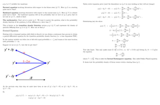
Dynamics of Vasicek Model
The Vasicek model
drt = (r rt) dt + dWt
is an example of a Mean Reverting Process - an important property of interest rates. refers to the
reversion rate (also called the speed of reversion) and r denotes the mean rate.
acts like a spring. Mean reversion means that a process which increases has a negative trend ( pulls
it down to a mean level r), and when rt decreases on average pulls it back up to r:
In discrete time we can approximate this by writing (as earlier)
ri+1 = ri + (r ri) t +
p
t
0
0.2
0.4
0.6
0.8
1
1.2
0 0.5 1 1.5 2 2.5 3 3.5
To gain an understanding of the properties of this model, look at dr in the absence of randomness
dr = (r r) dt
Z
dr
(r r)
=
Z
dt
r (t) = r + k exp ( kt)
So controls the rate of exponential decay.
One of the disadvantages of the Vasicek model is that interest rates can become negative. The Cox Ingersoll
Ross (CIR) model is similar to the above SDE but is scaled with the interest rate:
drt = (r rt) dt +
p
rtdWt:
If rt ever gets close to zero, the amount of randomness decreases, i.e. di¤usion ! 0; therefore the drift
dominates, in particular the mean rate.
12

122. Producing Standardized Normal Random Variables
Consider the RAND() function in Excel that produces a uniformly distributed random number over 0 and
1; written Unif[0;1]: We can show that for a large number N,
lim
N!1
r
12
N
N
P
1
Unif[0;1]
N
2
N (0; 1) :
Introduce Ui to denote a uniformly distributed random variable over [0; 1] and sum up. Recall that
E [Ui] = 1
2
V [Ui] = 1
12
The mean is then
E
N
P
i=1
Ui = N=2
so subtract o¤ N=2; so we examine the variance of
N
P
1
Ui
N
2
V
N
P
1
Ui
N
2
=
N
P
1
V [Ui]
= N=12
As the variance is not 1, write
V
N
P
1
Ui
N
2
for some 2 R: Hence 2 N
12
= 1 which gives =
p
12=N which normalises the variance. Then we achieve
the result r
12
N
N
P
1
Ui
N
2
:
Rewrite as
N
P
1
Ui N 1
2
q
1
12
p
N
:
and for N ! 1 by the Central Limit Theorem we get N (0; 1)
13
Generating Correlated Normal Variables
Consider two uncorrelated standard Normal variables 1 and 2 from which we wish to form a correlated
pair 1; 2 ( N (0; 1)), such that E [ 1 2] = : The following scheme can be used
1. E [1] = E [2] = 0 ; E [2
1] = E [2
2] = 1 and E [12] = 0 (* 1; 2 are uncorrelated) :
2. Set 1 = 1 and 2 = 1 + 2 (i.e. a linear combination).
3. Now
E [ 1 2] = = E [1 ( 1 + 2)]
E [1 ( 1 + 2)] =
E 2
1 + E [12] = ! =
E 2
2 = 1 = E ( 1 + 2)2
= E 2
2
1 + 2
2
2 + 2 12
= 2
E 2
1 + 2
E 2
2 + 2 E [12] = 1
2
+ 2
= 1 ! =
p
1 2
4. This gives 1 = 1 and 2 = 1+
p
1 2 2 which are correlated standardized Normal variables.
14

123. Transition Probability Density Functions for Stochastic Di¤erential Equa-
tions
To match the mean and standard deviation of the trinomial model with the continuous-time random walk
we choose the following de…nitions for the probabilities
+
(y; t) =
1
2
t
y2
B2
(y; t) + A (y; t) y ;
(y; t) =
1
2
t
y2
B2
(y; t) A (y; t) y
We …rst note that the expected value is
+
( y) + ( y) + 1 +
(0)
= +
y
We already know that the mean and variance of the continuous time random walk given by
dy = A (y; t) dt + b (y; t) dW
is, in turn,
E [dy] = Adt
V [dy] = B2
dt:
So to match the mean requires
+
y = A t
The variance of the trinomial model is E [u2
] E2
[u] and hence becomes
( y)2 +
+ + 2
( y)2
= ( y)2 +
+ + 2
:
We now match the variances to get
( y)2 +
+ + 2
= B2
t
First equation gives
+
= + A t
y
which upon substituting into the second equation gives
( y)2
+ + +
2
= B2
t
where = A t
y
: This simpli…es to
2 + 2
= B2 t
( y)2
which rearranges to give
=
1
2
B2 t
( y)2 + 2
=
1
2
B2 t
( y)2 + A t
y
2
A t
y
=
1
2
t
( y)2 B2
+ A2
t A y
15
t is small compared with y and so
=
1
2
t
( y)2 B2
A y :
Then
+
= + A t
y
=
1
2
t
( y)2 B2
+ A y :
Note
+
+ ( y)2
= B2
t
16

124. Derivation of the Fokker-Planck/Forward Kolmogorov Equation
Recall that y0
; t0
are futures states.
We have p (y; t; y0
; t0
) =
(y0
+ y; t0
t) p (y; t; y0
+ y; t0
t)
+ 1 (y0
; t0
t) +
(y0
; t0
t) p (y; t; y0
; t0
t)
+ +
(y0
y; t0
t) p (y; t; y0
y; t0
t)
Expand each of the terms in Taylor series about the point y0
; t0
to …nd
p (y; t; y0
+ y; t0
t) = p (y; t; y0
; t0
) + y
@p
@y0
+
1
2
y2 @2
p
@y02
t
@p
@t0
+ :::::;
p (y; t; y0
; t0
t) = p (y; t; y0
; t0
) t
@p
@t0
+ :::;
p (y; t; y0
y; t0
t) = p (y; t; y0
; t0
) y
@p
@y0
+
1
2
y2 @2
p
@y02
t
@p
@t0
+ :::::;
+
(y0
y; t0
t) = +
(y0
; t0
) y
@ +
@y0
+
1
2
y2 @2 +
@y02
t
@ +
@t0
+ ::::::;
+
(y0
; t0
t) = +
(y0
; t0
) t
@ +
@t0
+ ::::::;
(y0
+ y; t0
t) = (y0
; t0
) + y
@
@y0
+
1
2
y2 @2
@y02
t
@
@t0
+ ::::::;
(y0
; t0
t) = (y0
; t0
) t
@
@t0
+ ::::::;
Substituting in our equation for p (y; t; y0
; t0
), ignoring terms smaller than t, noting that y O
p
t ;
gives
@p
@t0
=
@
@y0
1
y
+
p +
1
2
@2
@y02
+
p :
Noting the earlier results
A =
( y)2
t
1
y
+
;
B2
=
( y)2
t
+
+
gives the forward equation
@p
@t0
=
1
2
@2
@y02
B2
(y0
; t0
) p
@
@y0
(A (y0
; t0
) p)
The initial condition used is
p (y; t; y0
; t0
) = (y0
y)
17
As an example consider the important case of the distribution of stock prices. Given the random walk for
equities, i.e. Geometric Brownian Motion
dS
S
= dt + dW:
So A (S0
; t0
) = S0
and B (S0
; t0
) = S0
: Hence the forward becomes
@p
@t0
=
1
2
@2
@S02
2
S02
p
@
@S0
( S0
p) :
This can be solved with a starting condition of S0
= S at t0
= t to give the transition pdf
p (S; t; S0
; T) =
1
S0
p
2 (t0 t)
e (log(S=S0)+( 1
2
2
)(t0 t))
2
/2 2(t0 t)
:
More on this and solution technique later, but note that a transformation reduces this to the one dimen-
sional heat equation and the similarity reduction method which follows is used.
The Steady-State Distribution
As the name suggests ’
steady state’ refers to time independent. Random walks for interest rates and
volatility can be modelled with stochastic di¤erential equations which have steady-state distributions. So
in the long run, i.e. as t0
! 1 the distribution p (y; t; y0
; t0
) settles down and becomes independent of the
starting state y and t: The partial derivatives in the forward equation now become ordinary ones and the
unsteady term @p
@t0 vanishes.
The resulting forward equation for the steady-state distribution p1 (y0
) is governed by the ordinary di¤er-
ential equation
1
2
d2
dy02
B2
p1
d
dy0
(Ap1) = 0:
Example: The Vasicek model for the spot rate r evolves according to the stochastic di¤erential equation
dr = (r r) dt + dW
Write down the Fokker-Planck equation for the transition probability density function for the interest rate
r in this model.
Now using the steady-state version for the forward equation, solve this to …nd the steady state probability
distribution p1 (r0
) ; given by
p1 = 1
r
exp 2 (r0
r)
2
:
Solution:
For the SDE dr = (r r) dt+ dW where drift = (r r) and di¤usion is the Fokker Planck equation
becomes
@p
@t0
=
1
2
2 @2
p
@r0 2
@
@r0
((r r0
) p)
where p = p (r0
; t0
) is the transition PDF and the variables refer to future states. In the steady state
case, there is no time dependency, hence the Fokker Planck PDE becomes an ODE with
1
2
2 d2
p1
dr2
d
dr
((r r) p1) = 0
18

125. p1 = p1 (r) : The prime notation and subscript have been dropped simply for convenience at this stage.
To solve the steady-state equation:
Integrate wrt r
1
2
2 dp
dr
((r r) p) = k
where k is a constant of integration and can be calculated from the conditions, that as r ! 1
(
dp
dr
! 0
p ! 0
) k = 0
which gives
1
2
2 dp
dr
= ((r r) p) ;
a …rst order variable separable equation. So
1
2
2
Z
dp
p
=
Z
((r r)) dr !
1
2
2
ln p = rr
r2
2
+ C , C is arbitrary.
Rearranging and taking exponentials of both sides to give
p = exp 2
2 rr
r2
2
+ D = E exp 2
2
r2
2
rr
Complete the square to get
p = E exp 2 (r r)2
r2
p1 = A exp 2 (r0
r)
2
:
There is another way of performing the integration on the rhs. If we go back to
R
(r r) dr and write
as Z
1
2
d
dr
(r r)2
dr =
2
(r r)2
to give
1
2
2
ln p =
2
(r r)2
+ C:
Now we know as p1 is a PDF
Z 1
1
p1 dr0
= 1 !
A
Z 1
1
exp 2 (r0
r)
2
dr0
= 1
A few (related) ways to calculate A. Now use the error function, i.e.
Z 1
1
e x2
dx =
p
So put
x =
q
2 (r0
r) ! dx =
q
2 dr0
19
which transforms the integral above
A
p
Z 1
1
e x2
dx = 1 ! A
r
= 1
therefore
A = 1
r
:
This allows us to …nally write the steady-state transition PDF as
p1 = 1
r
exp 2 (r0
r)
2
:
The backward equation is obtained in a similar way to the forward
p (y; t; y0
; t0
) =
+
(y; t) p (y + y; t + t; y0
; t0
)
+ 1 (y; t) +
(y; t) p (y; t + t; y0
; t0
)
+ (y; t) p (y y; t + t; y0
; t0
)
and expand using Taylor. The resulting PDE is
@p
@t
+
1
2
B2
(y; t)
@2
p
@y2
+ A (y; t)
@p
@y
= 0:
20

126. Review of Module 1
The Binomial Model
The model has made option pricing accessible to MBA students and …nance practitioners preparing for
the CFA
R
: It is a very useful tool for conveying the ideas of delta hedging and no arbitrage, in addition
to the subtle concept of risk neutrality and option pricing. Here the model is considered in a slightly more
mathematical way.
The basic assumptions in option pricing theory consist of two forms, key:
Short selling allowed
No arbitrage opportunities
and relaxable
Frictionless markets
Perfect liquidity
Known volatility and interest rates
No dividends on the underlying
The key assumptions underlying the binomial model are:
an asset value changes only at discrete time intervals
an asset’
s worth can change to one of only two possible new values at each time step.
The one period model - Replication
Another way of looking at the Binomial model is in terms of replication: we can replicate the option
using only cash (or bonds) and the asset. That is, mathematically, simply a rearrangement of the earlier
equations. It is, nevertheless a very important interpretation.
In one time step:
1. The asset moves from S0 = s to S1 = su or S1 = sd:
2. An option X pays o¤ xu if the asset price is su and xd if the price is sd:
3. There is a bond market in which a pound invested today is continuously compounded at a constant
(risk-free) rate r and becomes er
; one time-step later.
Now consider a portfolio of bonds and assets which at time t = 0; will have an initial value of
V0 = S0 +
Now with this money we can buy or sell bonds or stocks in order to obtain a new portfolio at time-step 1:
Can we construct a hedging strategy which will guarantee to pay o¤ the option, whatever happens to the
asset price?
1
The Hedging Strategy
We arrange the portfolio so that its value is exactly that of the required option pay-out at the terminal
time regardless of whether the stock moves up or down.
This is because having two unknowns ; ; the amount of stock and bond, and we wish to match the two
possible terminal values, xu; xd; the option payo¤s. Thus we need to have
xu = su + er
;
xd = sd + er
:
Solving for ; we have
=
xu xd
su sd
= e r xdsu xusd
su sd
This is a hedging strategy.
At time step 1; the value of the portfolio is
V1 =
xu
xd
if S1 = su
if S1 = sd
This is the option payo¤. Thus, given V0 = S0 + we can construct the above portfolio which has the
same payo¤ as the option. Hence the price for the option must be V0: Any other price would allow arbitrage
as you could play this hedging strategy, either buying or selling the option, and make a guaranteed pro…t.
Thus the fair, arbitrage-free price for the option is given by
V0 = ( S0 + )
=
xu xd
su sd
s + e r xdsu xusd
su sd
= e r er
s sd
su sd
xu +
su er
s
su sd
xd :
De…ne
q =
er
s sd
su sd
;
then we conclude that
V0 = e r
(qxu + (1 q) xd)
where
0 q 1:
We can think of q as a probability induced by insistence on no-arbitrage, i.e. the so-called risk-neutral
probability. It has nothing to do with the real probabilities of su and sd occurring; these are p and 1 p;
in turn.
The option price can be viewed as the discounted expected value of the option pay-o¤ with respect to the
probabilities q;
V0 = e r
(qxu + (1 q) xd)
= Eq e r
X :
2

127. The fact that the risk neutral/fair value (or q value) of a call is less than the expected value of the call
(under the real probability p), is not a puzzle.
Pricing a call using the real probability, p, you will probably make a pro…t, but you might also might make
a loss. Pricing an option using the risk-neutral probability, q, you will certainly make neither a pro…t nor
a loss.
Assume an asset which has value S and during a time step t can either rise to uS or fall to vS with
0 v 1 u: So as earlier probabilities of a rise and fall in turn are p and 1 p:
uS
%
S
vS
| {z }
t
V +
uS
%
V S
V vS
| {z }
t
Also set uv = 1 so that after an up and down move, the asset returns to S: Hence a recombining tree.
To implement the Binomial model we need a model for asset price evolution to predict future possible spot
prices. So use
S = S t + S
p
t;
i.e. discrete version of GBM: The 3 constants u; v; p are chosen to give the binomial model the same drift
and di¤usion as the SDE. For the correct drift, choose
pu + (1 p) v = e t
(a)
and for the correct standard deviation set
pu2
+ (1 p) v2
= e(2 + 2
) t
(b)
u (a) + v (a) gives
(u + v) e t
= pu2
+ uv puv + pvu + v2
pv2
:
Rearrange to get
(u + v) e t
= pu2
+ + (1 p) v2
+ uv
and we know from (b) that pu2
+ (1 p) v2
= e(2 + 2
) t
and uv = 1: Hence we have
(u + v) e t
= e(2 + 2
) t
+ 1 )
(u + v) = e t
+ e( + 2
) t
:
Now recall that the quadratic equation ax2
+ bx + c = 0 with roots and has
+ =
b
a
; =
c
a
:
3
We have
(u + v) = e t
+ e( + 2
) t b
a
uv = 1
c
a
hence u and v satisfy
(x u) (x v) = 0
to give the quadratic
x2
(u + v) x + uv = 0 )
x =
(u + v)
q
(u + v)2
4uv
2
so with u 1
u =
1
2
e t
+ e( + 2
) t
+
1
2
q
(e t + e( + 2) t)
2
4
In this model, the hedging argument gives
V +
uS = V vS
which leads to =
V +
V
(u v) S
: Because all other terms are known choose to eliminate risk.
We know tomorrow’
s option value therefore price today is tomorrow’
s value discounted for interest rates
V S =
1
1 + r t
V +
uS
so (1 + r t) (V S) = V +
uS and replace using the de…nition of above
(1 + r t) V = V + v + 1 + r t
(u v)
+ V
u 1 r t
(u v)
where the risk-neutral probabilities are
q =
v + 1 + r t
(u v)
1 q =
u 1 r t
(u v)
:
So (1 + r t) V = V +
q + V (1 q) :
Finally we have
V =
V +
V
(u v)
+
uV vV +
(1 + r t) (u v)
q =
er t
v
(u v)
4

128. The Continuous Time Limit
Performing a Taylor expansion around t = 0 we have
u
1
2
(1 t + ) + 1 + + 2
t + +
1
2
e 2 t
+ 2e
2 t
+ e2( + 2
) t
4
1
2
= 1 +
1
2
2
t + +
1
2
1 2 t + 2 + 2 2
t + 1 + 2 t + 2 2
t 4 +
= 1 +
1
2
2
t + +
1
2
4 2
t +
1
2
Ignoring the terms of order t
3
2 and higher we get the result
= 1 + t
1
2 +
1
2
2
t +
Since uv = 1 this implies that v = u 1
. Using the expansion for u obtained earlier we have
v = 1 + t
1
2 +
1
2
2
t +
1
= 1 + t
1
2 1 +
1
2
t
1
2
1
= 1 t
1
2 1 +
1
2
t
1
2 + t
1
2 1 +
1
2
t
1
2
2
+
!!
= 1 t
1
2
1
2
2
t + 2
t +
= 1 t
1
2 +
1
2
2
t
So we have
u 1 +
p
t +
1
2
2
t
v 1
p
t +
1
2
2
t
So to summarise we can write
u = e
p
t
v = e
p
t
q =
er t
v
(u v)
and use these to build the asset price tree using u and v; and then value the option backwards from T
using
er t
V (S; t) = qV (uS; t + t) + (1 q) V (vS; t + t)
and at each stage the headge ratio is obtained using
=
V +
V
(u v) S
=
V (uS; t + t) V (vS; t + t)
(u v) S
5
Note that
=
V +
V
(u v) S
2
p
tS @V
@S
2
p
tS
=
@V
@S
Now expand
V +
= V (uS; t + t) V + t
@V
@t
+
p
tS
@V
@S
+ 1
2
2
tS2 @2
V
@S2
;
V = V (vS; t + t) V + t
@V
@t
p
tS
@V
@S
+ 1
2
2
tS2 @2
V
@S2
:
Then
V =
V +
V
(u v)
+
uV vV +
(1 + r t) (u v)
=
2
p
tS
2
p
t
@V
@S
+
1 +
p
t V 1
p
t V +
(1 + r t) 2
p
t
Rearranging to give
(1 + r t) 2
p
tV = 2
p
tS (1 + r t)
@V
@S
+ V V +
+
p
t V + V +
;
and so
(1 + r t) 2
p
tV = 2
p
tS (1 + r t)
@V
@S
2
p
tS
@V
@S
+
2
p
t V + 1
2
2
tS2 @2
V
@S2
+ t
@V
@t
;
(1 + r t) V = S (1 + r t)
@V
@S
S
@V
@S
+ V + 1
2
2
tS2 @2
V
@S2
+ t
@V
@t
;
divide through by t and allow t ! 0
rV = rS
@V
@S
+ 1
2
2
S2 @2
V
@S2
+
@V
@t
and hence the Black-Scholes Equation.
6

129. Probability
Probability theory provides the necessary structure to model the uncertainty that is central to …nance and
is the chief reason for its powerful in‡
uence in mathematical …nance. Any formal discussion of random
variables requires de…ning the triple ( ; F; P) ; as it forms the foundation of the probabilistic universe. This
three-tuple is called a probability space and comprises of
1. the sample space
2. the …ltration F
3. the probability measure P
Basic set theoretic notions have special interpretations in probability theory. Here are some
The complement in of the event A; written Ac
is interpreted as not A and occurs i¤ A does
not occur.
The union A [ B of two events A and B is the event at least one of A or B occurs.
The intersection A B of two events A and B is the event both A and B occur. Events A and
B are said to be mutually exclusive if they are disjoint, A B = ;; and so both cannot occur
together.
The inclusion relation A B means the occurrence of A implies the occurrence of B.
Example The daily closing price of a risky asset, e.g. share price on the FTSE100. Over the course of a
year (252 business days)
= fS1; S2; S3; : : : ; S252g
We could de…ne an event e.g. = fSi : Si 110g
Outcomes of experiments are not always numbers, e.g. 2 heads appearing; picking an ace from a deck of
cards, or the coin ‡
ipping example above. We need some way of assigning real numbers to each random
event. Random variables assign numbers to events. Thus a random variable (RV) X is a function which
maps from the sample space to the set of real numbers
X : ! 2 ! R;
i.e. it associates a number X (!) with each outcome !: A more robust de…nition will follow.
Consider the example of tossing a coin and suppose we are paid £ 1 for each head and we lose £ 1 each time
a tail appears. We know that P (H) = P (T) = 1
2
: So now we can assign the following outcomes
P (1) =
1
2
; P ( 1) =
1
2
7
Mathematically, if our random variable is X; then
X =
+1 if H
1 if T
or using the notation above X : ! 2 fH,Tg ! f 1; 1g :
Returning to the coin tossing game we see the sample space has two events: !1 = Head; !2 = Tail.
So now
= f!1; !2g
And the PL from this game is a RV X de…ned by
X (!1) = +1
X (!2) = 1
= f!1; !2g ) 2 = f;; f 1g ; f+1g ; f 1; +1gg.
In a multi-period market, information about the market is revealed in stages. The n period Binomial
model demonstrates the way this information becomes available.
Some events may be completely determined by the end of the …rst trading period, others by the end of the
second or third, and others will only be available at the termination of all trading. These events can be
classi…ed in the following way; consider time t T; de…ne
Ft = fall events determined in the …rst t trading periodsg
The binomial stock price model is a discrete time stochastic model of a stock price process in which a
…ctitious coin is tossed and the stock price dynamics depend on the outcome of the coin tosses e.g. a Head
means the stock rises by one unit, a tail means the stock falls by that same amount. Start by introducing
some new probabilistic terminology and concepts.
Suppose T := f0; 1; 2; :::; ng represents a discrete time set.
The sample space = n; the set of all outcomes of n coin tosses; each sample point ! 2 is of length
n; written as ! = !1!2::::!n; where each f!t : t 2 Tg is either U (due to a Head) or D (due to a Tail),
representing the outcome of the tth
coin toss. So e.g. three coin tosses would give a sample path ! = !1!2!3
of length 3:
We are interested in a stochastic process due to the dynamic nature of asset prices.
Suppose before the markets open we guess the possible outcomes of the stock price, this will give us our
sample space. The sample path will tell us what just happened. Consider a stock price which over the
next time step can go up U or go down D.
8

130. 1 = fU; Dg :
21
outcomes
! = !1 length 1
Then a two time period model looks like
So the sample space at the end of two time periods is
2 = fUU; UD; DU; DDg :
22
outcomes
! = !1!2 length 2
For this experiment a sample path or trajectory would be one realisation e.g. DU or DD: Generally in
probability theory, the sample space is of greater interest. As the number of time periods becomes larger
and larger it becomes increasingly di¢ cult to track all of the possible outcomes and corresponding sample
space generated through time, i.e. 1; 2; 3; :::; t; t+1;::::
The …ltration, F, is an indication of how an increasing family of events builds up over time as more results
become available, it is much more than just a family of events. The …ltration, F is a set formed of all
possible combinations of events A ; their unions and complements. So for example if we want to know
what events can occur we are also interested in what cannot happen. The …ltration F is an object in
Measure Theory called a algebra (also called a …eld). algebras can be interpreted as records of
information. Measure theory was brought to probability by Kolmogorov.
Now let F be the non-empty set of all subsets of ; then F 2 is a algebra (also called a …eld),
that is, a collection of subsets of with the properties:
9
1. ; 2 F
2. If A F then Ac
F (closed under complements)
3. If the sequence Ai F 8i 2 N =)
S1
i=1 Ai F (closed under countable unions)
The second property also implies that F. In addition
T1
i=1 Ai F. The pair ( ; F) is called a
measurable space.
Key Fact: For 0 t1 t2 ::: T;
Ft1 Ft2 ::: FT F
Since we consider that information gets constantly recorded and accumulates up until the end of the
experiment T without ever getting lost or forgotten, it is only logical that with the passage of time the
…ltration increases.
In general it is very di¢ cult to describe explicitly the …ltration. In the case of (say) the binomial model,
this can be done. Consider a 3-period binomial model. At the end of each time period new information
becomes available, allowing us to predict the stock price trajectory.
Example Consider a 3-period binomial model. At the end of each period, new information becomes
available to help us predict the actual stock trajectory. So take n = 3; = 3; given by the …nite set
3 = fUUU; UUD; UDU; UDD; DUU; DUD; DDU; DDDg ;
the set of all possible outcomes of three coin tosses. At time t = 0, before the start of trading we only have
the trivial …ltration
F0 = f ; ;g
since we do not have any information regarding the trajectory of the stock. The trivial algebra F0
contains no information: knowing whether the outcome ! of the two tosses is in ;; (it is not) and whether
it is in (it is) tells you nothing about !, in accordance with the idea that at time zero one knows nothing
10

131. about the eventual outcome ! of the three coin tosses. All one can say is that ! =
2 ; and ! 2 and so
F0 = f ; ;g.
Now de…ne the following two subsets of :
AU = fUUU; UUD; UDU; UDDg ; AD = fDUU; DUD; DDU; DDDg :
We see AU is the subset of outcomes where a Head appears on the …rst throw, AD is the subset of outcomes
where a Tail lands on the …rst throw. After the …rst trading period t = 1,(11am) we know whether the
initial move was an up move or down move. Hence
F1 = f ; ;; AU ; ADg
De…ne also
AUU = fUUU; UUDg ; AUD = fUDU; UDDg ;
ADU = fDUU; DUDg ; ADD = fDDU; DDDg
corresponding to the events that the …rst two coin tosses result in HH; HT; TH; TT respectively. This
is the information we have at the end of the 2nd trading period t = 2,(1 pm). This means at the end of
the second trading period we have accumulated increasing information. Hence
F2 = f ; ;; AU ; AD; AUU ; AUD; ADU ; ADD + all unions of theseg ;
which can be written as follows
F2 = f ; ;; AU ; AD; AUU ; AUD; ADU ; ADD
AUU [ ADU ; AUU [ ADD; AUD [ ADU ; AUD [ ADD
Ac
UU ; Ac
UD; Ac
DU ; Ac
DDg
We see
F0 F1 F2
Then F2 is a algebra which contains the information of the …rst two tosses of the information up to
time 2. This is because, if you know the outcome of the …rst two tosses, you can say whether the outcome
! 2 of all three tosses satis…es ! 2 A or ! =
2 A for each A 2 F2:
Similarly, F3 F; the set of all subsets of ; contains full information about the outcome of all three
tosses. The sequence of increasing algebras F = fF0; F1; F2; F3g is a …ltration.
Adapted Process A stochastic process St is said to be adapted to the …ltration Ft (or Ft measurable or
Ft adapted) if the value of S at time t is known given the information set Ft:
We place a probability measure P on f ; Fg : P is a special type of function, called a measure which
assigns probabilities to subsets (i.e. the outcomes); the theory also comes from Measure Theory. Whereas
cumulative density functions (CDF) are de…ned on intervals such as R; probability measures are de…ned
on general sets, giving greater power, generalisation and ‡
exibility. A probability measure P is a function
mapping P : F ! [0; 1] with the properties
(i) P ( ) = 1;
(ii) if A1; A2; :::: is a sequence of disjoint sets in F; then P (
S1
k=1 Ak) =
1
X
k=1
P (Ak) :
11
Example Recall the usual coin toss game with the earlier de…ned results. As the outcomes are equiprobable
the probability measure de…ned as P (!1) = 1
2
= P (!2) :
The interpretation is that for a set A 2F there is a probability in [0; 1] that the outcome of a random
experiment will lie in the set A: We think of P (A) as this probability. The A 2F is called an event. For
A 2F we can de…ne
P (A) :=
X
!2A
P (!) ; (*)
as A has …nitely many elements. Letting the probability of H on each coin toss be p 2 (0; 1) ; so that the
probability of T is q = 1 p. For each ! = (!1; !2; : : : !n) 2 we de…ne
P (!) := pNumber of H in !
qNumber of T in !
:
Then for each A 2F we de…ne P (A) according to ( ) :
In the …nite coin toss space, for each t 2 T let Ft be the algebra generated by the …rst t coin tosses.
This is a algebra which encapsulates the information one has if one observes the outcome of the …rst
t coin tosses (but not the full outcome ! of all n coin tosses). Then Ft is composed of all the sets A such
that Ft is indeed a algebra, and such that if the outcome of the …rst t coin tosses is known, then we
can say whether ! 2 A or ! =
2 A; for each A 2 Ft: The increasing sequence of algebras (Ft)t2T is an
example of a …ltration. We use this notation when working in continuous time.
When moving to continuous time we will write (Ft)t2[0;T] :
If we are concerned with developing a more measure theory based rigorous approach then working structures
such as algebras becomes more important - so we do not need to worry too much about this in our
…nancial mathematics setting.
We can compute the probability of any event. For instance,
P (AU ) = P (H on …rst toss) = P fUUU; UUD; UDU; UDDg
= p3
+ 2p2
q + pq2
= p;
and similarly P (AT ) = q: This agrees with the mathematics and our intuition.
Explanation of probability measure: If the number of basic events is very large we may prefer to
think of a continuous probability distribution. As the number of discrete events tends to in…nity, the
probability of any individual event usually tends to zero. In terms of random variables, the probability
that the random variable X takes a given value tends to zero.
So, the individual probabilities pi are no longer useful. Instead we have a probability density function p (x)
with the property that
Pr (x X x + dx) = p (x) dx
for any in…nitesimal interval of length dx (think of this as a limiting process starting with a small interval whos
It is also called a density because it is the probability of …nding X on an interval of length dx divided by
the length of the interval. Recall that the following are analogous
Z 1
1
p (x) dx = 1
X
i
pi = 1:
12

132. The (cumulative) distribution function of a random variable is de…ned by
P (x) = Pr (X x) :
It is an increasing function of x with P ( 1) = 0 and P (1) = 1; note that 0 P (x) 1: It is related
to the density function by
p (x) =
dP (x)
dx
provided that P (x) is di¤erentiable. Unlike P (x) ; p (x) may be unbounded or have singularities such as
delta functions.
P is the probability measure, a special type of function, called a measure, assigning probabilities to
subsets (i.e. the outcomes); the mathematics emanates from Measure Theory. Probability measures are
similar to cumulative density functions (CDF); the chief di¤erence is that where PDFs are de…ned on
intervals (e.g. R), probability measures are de…ned on general sets. We are now concerned with mapping
subsets on to [0; 1] : The following de…nition of the expectation has been used
E [h (X)] =
Z
R
h (x) p (x) dx
=
Z
R
h (x) dP (x)
We now write as a Lebesgue integral with respect to the measure P
EP
[h (X (!))] =
Z
h (!) P (d!) :
So integration is now done over the sample space (and not intervals).
If fWt : t 2 [0; T]g is a Brownian motion or any general stochastic process fSn : n = 0; :::; Ng. The proba-
bility space ( ; F; P) is the set of all paths (continuous functions) and P is the probability of each path.
Example Recall the usual coin toss game with the earlier de…ned results. As the outcomes are equiprobable
the probability measure de…ned as P (!1) = 1
2
= P (!2) :
There is a very powerful relation between expectations and probabilities. In our formula for the expectation,
choose f (X) to be the indicator function 1x2A for a subset A de…ned
1x2A =
1
0
if x 2 A
if x =
2 A
i.e. when we are in A; the indicator function returns 1.
The expectation of the indicator function of an event is the probability associated with this event:
E [1X2A] =
Z
1x2AdP
=
Z
A
dP+
Z
nA
dP
=
Z
A
dP
= P (A)
which is simply the probability that the outcome X 2 A:
13
Conditional Expectations
What makes a conditional expectation di¤erent (from an unconditional one) is information (just as in
the case of conditional probability). In our probability space, ( ; F; P) information is represented by the
…ltration F; hence a conditional expectation with respect to the (usual information) …ltration seems a
natural choice.
Y = E [Xj F]
is the expected value of the random variable conditional upon the …ltration set F: In general
In general Y will be a random variable
Y will be adapted to the …ltration F:
Conditional expectations have the following useful properties: If X; Y are integrable random variables and
a; b are constants then
1. Linearity:
E [aX + bY j F] = aE [Xj F] + bE [Y j F]
2. Tower Property (i.e. Iterated Expectations): if G F
E [E [Xj F]j G] = E [Xj G] :
This property states that if taking iterated expectations with respect to several levels of information,
we may as well take a single expectation subject to the smallest set of available information. The
special case is
E [E [Xj F]] = E [X] :
3. Taking out what is known: X is F adapted, then the value of X is know once we know F.
Therefore
E [Xj F] = X:
and hence by extension if X is F measurable, but not Y then
E [XY j F] = XE [Y j F] :
4. Independence: X is independent of F; then knowing F is of no use in predicting X
E [Xj F] = E [X] :
5. Positivity: If X 0 then E [Xj F] 0:
6. Jensen’
s inequality: Let f be a convex function, then
f (E [Xj F]) fE [f (X)j F]
14

133. Solving the Di¤usion Equation
The Heat/Di¤usion equation
Consider the equation
@u
@t
= c2 @2
u
@x2
for the unknown function u = u (x; t) ; c2
is a positive constant: The idea is to obtain a solution in terms
of Gaussian curves. So u (x; t) represents a probability density.
We assume a solution of the following form exists:
u (x; t) = t 1=2
f
x
t1=2
and the non-dimensional variable
=
x
t1=2
which allows us to obtain the following derivatives
@
@x
= t 1=2
;
@
@t
=
1
2
xt 3=2
we can now say
u (x; t) = t 1=2
f ( )
therefore
@u
@x
=
@u
@
@
@x
= t 1=2
f0
( )
1
t1=2
= t 1
f0
( )
@2
u
@x2
=
@
@x
@u
@x
=
@
@x
t 1
f0
( ) = t 3=2
f00
( )
@u
@t
= t 1=2 @
@t
f ( )
1
2
t 3=2
f ( )
= t 1=2 1
2
xt 3=2
f0
( )
1
2
t 3=2
f ( )
=
1
2
t 3=2
f0
( )
1
2
t 3=2
f ( )
and then substituting
@u
@t
=
1
2
t 3=2
( f0
( ) + f ( ))
@2
u
@x2
= t 3=2
f00
( )
gives
1
2
t 3=2
( f0
( ) + f ( )) = c2
t 3=2
f00
( )
simplifying to the ODE
1
2
(f + f0
) = c2
f00
:
We have an exact derivative on the left hand side, i.e.
d
d
( f) = f + f0
, hence
1
2
d
d
( f) = c2
f00
15
and we can integrate once to get
1
2
( f) = c2
f0
+ K:
We set K = 0 in order to get the correct solution, i.e.
1
2
( f) = c2
f0
which can be solved as a simple …rst order variable separable equation:
f ( ) = A exp 1
4c2
2
A is a normalizing constant, so write
A
Z
R
exp 1
4c2
2
d = 1:
Now substitute s = =2c; so 2cds = d
2cA
Z
R
exp s2
ds
| {z }
=
p
= 1;
which gives A =
1
2c
p : Returning to
u (x; t) = t 1=2
f ( )
becomes
u (x; t) =
1
2c
p
t
exp
x
2
4tc2
!
:
Hence the random variable x is Normally distributed with mean zero and standard deviation c
p
2t:
16

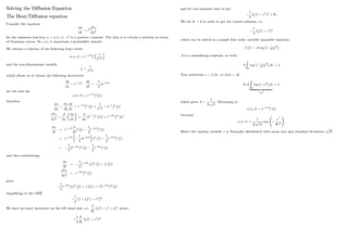
134. Applied Stochastic Calculus
Stochastic Process
The evolution of …nancial assets is random and depends on time. They are examples of stochastic processes
which are random variables indexed (parameterized) with time.
If the movement of an asset is discrete it is called a random walk. A continuous movement is called a
di¤usion process. We will consider the asset price dynamics to exhibit continuous behaviour and each
random path traced out is called a realization.
We need a de…nition and set of properties for the randomness observed in an asset price realization, which
will be Brownian Motion.
This is named after the Scottish Botanist who in 1827, while examining grains of pollen of the plant Clarkia
pulchella suspended in water under a microscope, observed minute particles, ejected from the pollen grains,
executing a continuous …dgety motion. In 1900 Louis Bachelier was the …rst person to model the share price
movement using Brownian motion as part of his PhD. Five years later Einstein used Brownian motion to
study di¤usions. In 1920 Norbert Wiener, a mathematician at MIT provided a mathematical construction
of Brownian motion together with numerous results about the properties of Brownian motion - in fact he
was the …rst to show that Brownian motion exists and is a well de…ned entity! Hence Wiener process is
also used as a name for this.
Construction of Brownian Motion and properties
We construct Brownian motion using a simple symmetric random walk. De…ne a random variable
Zi =
1
1
if H
if T
Let
Xn =
n
X
i=1
Zi
which de…nes the marker’
s position after the nth
toss of the game. This is conditional upon the marker
starting at position X = 0; so at each time-step moves one unit either to the left or right with equal
probability. Hence the distribution is binomial with
mean =
1
2
(+1) +
1
2
( 1) = 0
variance =
1
2
(+1)2
+
1
2
( 1)2
= 1
This can be approximated to a Normal distribution due to the Central Limit Theorem.
Is there a continuous time limit to this discrete random walk? Let’
s introduce time dependency. Take a
time period for our walk, say [0; t] and perform N steps. So we partition [0; t] into N time intervals, so
each step takes
t = t=N:
Speed up this random walk so let N ! 1: The problem with the original step sizes of 1 gives the variance
that is in…nite. We rescale the space step, keeping in mind the central limit theorem. Let
Y = N Z
17
for some N to be found, and let XN
n ; n = 0; :::; N such that XN
0 = 0; be the path/trajectory of the
random walk with steps of size N :
Thus we now have
E XN
n = 0; 8n
and
V XN
n = E
h
XN
n
2
i
= NE Y 2
= N 2
N E Z2
= N 2
N
1
2
+
1
2
=
t
t
2
N :
Obviously we must have 2
N = t = O (1) : Choosing 2
N = t = 1 gives
E X2
= V [X] = t:
As N ! 1; the symmetric random walk
n
XN
[tN]; t 2 [0; 1)
o
converges to a standard Brownian motion
fWt; t 2 [0; 1)g : So Wt N (0; dt) :
With t = n t we have
dWt
dt
= lim
t!0
Wt+ t Wt
t
! 1:
Quadratic Variation
Consider a function f (t) on the interval [0; T] : Discretising by writing t = idt and dt = T=N we can de…ne
the variation Vn
of f for n = 1; 2; :: as
Vn
[f] = lim
N!1
N 1
X
i=0
jfti+1 fti
jn
:
Of interest is the quadratic variation
Q [f] = lim
N!1
N 1
X
i=0
(fti+1 fti
)2
:
If f (t) has more than a …nite number of jumps or a singularity then Q [f] = 1:
For a Brownian motion on [0; T] we have
Q [Wt] = lim
N!1
N 1
X
i=0
(Wti+1 Wti
)2
= lim
N!1
N 1
X
i=0
(W ((i + 1) dt) W (idt))2
= lim
N!1
N 1
X
i=0
dt = lim
N!1
N 1
X
i=0
T
N
= T:
18

135. Suppose that f (t) is a di¤erentiable function on [0; T] : Then to leading order, we have
fti+1 fti
= f ((i + 1) dt) f (idt) f0
(ti) dt
so,
Q [f] lim
N!1
N 1
X
i=0
(f0
(ti) dt)
2
lim
N!1
dt
N 1
X
i=0
(f0
(ti))
2
dt
lim
N!1
T
N
Z T
0
(f0
(ti))
2
dt
= 0:
The quadratic variation of f (t) is zero. This argument remains valid even if f0
(t) has a …nite number of
jump discontinuities. Thus a Brownian motion, Wt; has at worst a …nite number of discontinuities, but
an in…nite number of discontinuities in its derivative, W0
t : It is continuous but not di¤erentiable, almost
everywhere. For us the important result is
dW2
t = dt
or more importantly we can write (up to mean square limit)
E dW2
t = dt:
Properties of a Wiener Process/Brownian motion
A stochastic process fWt : t 2 R+g is de…ned to be Brownian motion (or a Wiener process ) if
Brownian motion starts at zero, i.e. W0 = 0 (with probability one), i.e. P (W0 = 0) = 1:
Continuity - paths of Wt are continuous (no jumps) with probability 1. Di¤erentiable nowhere.
Brownian motion has independent Gaussian increments, with zero mean and variance equal to the
temporal extension of the increment. That is for each t 0 and s 0, Wt Ws is normal with mean
0 and variance jt sj ;
i.e.
Wt Ws N (0; jt sj) :
Coin tosses are Binomial, but due to a large number and the Central Limit Theorem we have a
distribution that is normal. Wt Ws has a pdf given by
p (x) =
1
p
2 jt sj
exp
x2
2 jt sj
More speci…cally Wt+s Wt is independent of Wt: This means if
0 t0 t1 t2 :::::
dW1 = W1 W0 is independent of dW2 = W2 W1
dW3 = W3 W2 is independent of dW4 = W4 W3
and so on
19
Also called standard Brownian motion if the above properties hold. More importantly is the result
(in stochastic di¤erential equations)
dW = Wt+dt Wt N (0; dt)
Brownian motion has stationary increments. A stochastic process (Xt)t 0 is said to be stationary if
Xt has the same distribution as Xt+h for any h 0. This can be checked by de…ning the increment
process I = (It)t 0 by
It := Wt+h Wt:
Then It N (0; h) ; and It+h = Wt+2h Wt+h N (0; h) have the same distribution. This is
equivalent to saying that the process (Wt+h Wt)h 0 has the same distribution 8t:
If we want to be a little more pedantic then we can write some of the properties above as
Wt NP
(0; t)
i.e. Wt is normally distributed under the probability measure P:
The covariance function for a Brownian motion at di¤erent times. Let can be calculated as follows.
If t s;
E [WtWs] = E (Wt Ws) Ws + W2
s
= E [Wt Ws]
| {z }
N(0;jt sj)
E [Ws] + E W2
s
= (0) 0 + E W2
s
= s
The …rst term on the second line follows from independence of increments. Similarly, if s t; then
E [WtWs] = t and it follows that
E [WtWs] = min ft; sg :
Brownian motion is a Martingale. Martingales are very important in …nance.
Think back to the way the betting game has been constructed. Martingales are essentially stochastic
processes that are meant to capture the concept of a fair game in the setting of a gambling environment
and thus there exists a rich history in the modelling of gambling games. Although this is a key example
area for us, they nevertheless are present in numerous application areas of stochastic processes.
Before discussing the Martingale property of Brownian motion formally, some general background infor-
mation.
A stochastic process fXn : 0 n 1g is called a P martingale with respect to the information …ltra-
tion Fn; and probability distribution P; if the following two properties are satis…ed
P1 EP
n [jXnj] 1 8 n 0
P2 EP
n [Xn+mj Fn] = Xn; 8 n; m 0
20

136. The …rst property is simply a technical integrability condition (…ne print), i.e. the expected value of the
absolute value of Xn must be …nite for all n: Such a …niteness condition appears whenever integrals de…ned
over R are used (think back to the properties of the Fourier Transform for example).
The second property is the one of key importance. This is another expectation result and states that the
expected value of Xn+m given Fn is equal to Xn for all non-negative n and m:
The symbol Fn denotes the information set called a …ltration and is the ‡
ow of information associated
with a stochastic process. This is simply the information we have in our model at time n: It is recognising
that at time n we have already observed all the information Fn = (X0; X1; ::::; Xn) :
So the expected value at any time in the future is equal to its current value - the information held at this
point it is the best forecast. Hence the importance of Martingales in modelling fair games. This property
is modelling a fair game, our future payo¤ is equal to the current wealth.
It is also common to use t to depict time
EP
t [MT j Ft] = Mt; t T
Taking expectations of both sides gives
Et [MT ] = Et [Mt] ; t T
so martingales have constant mean.
Now replacing the equality in P2 with an inequality, two further important results are obtained. A process
Mt which has
EP
t [MT j Ft] Mt
is called a submartingale and if it has
EP
t [MT j Ft] Mt
is called a supermartingale.
Using the earlier betting game as an example (where probability of a win or a loss was 1
2
)
submartingale - gambler wins money on average P (H) 1
2
supermartingale- gambler loses money on average P (H) 1
2
The above de…nitions tell us that every martingale is also a submartingale and a supermartingale. The
converse is also true.
For a Brownian motion, again where t T
EP
t [WT ] = EP
t [WT Wt + Wt]
= EP
t [WT Wt]
| {z }
N(0;jT tj)
+ EP
t [Wt]
The next step is important - and requires a little subtlety
The …rst term is zero. We are taking expectations at time t hence Wt is known, i.e. EP
t [Wt] = Wt: So
EP
t [WT ] = Wt:
21
Another important property of Brownian motion is that of a Markov process. That is if you observe the
path of the B.M from 0 to t and want to estimate WT where T t then the only relevant information
for predicting future dynamics is the value of Wt: That is, the past history is fully re‡
ected in the present
value. So the conditional distribution of Wt given up to t T depends only on what we know at t (latest
information).
Markov is also called memoryless as it is a stochastic process in which the distribution of future states
depends only on the present state and not on how it arrived there. It doesn’
t matter how you arrived at
your destination.
Let us look at an example. Consider the earlier random walk Sn given by
Sn =
n
X
i=1
Xi
which de…ned the winnings after n ‡
ips of the coin. The Xi’
s are IID with mean : now de…ne
Mn = Sn n :
We will demonstrate that Mn is a Martingale.
Start by writing
En [Mn+mj Fn] = En [Sn+m (n + m) ] :
So this is an expectation conditional on information at time n: Now work on the right hand side.
= En
n+m
X
i=1
Xi (n + m)
#
= En
n
X
i=1
Xi +
n+m
X
i=n+1
Xi
#
(n + m)
=
n
X
i=1
Xi + En
n+m
X
i=n+1
Xi
#
(n + m)
=
n
X
i=1
Xi + mEn [Xi] (n + m) =
n
X
i=1
Xi + m (n + m)
=
n
X
i=1
Xi n = Sn n
En [Mn+m] = Mn:
22

137. Functions of a stochastic variable and Stochastic Di¤erential Equations
In continuous time models, changes are (in…nitesimally) small. Calculus is used to analyse small changes,
hence an extension of ’
ordinary’deterministic calculus to variables governed by a di¤usion process.
Start by recalling a Taylor series expansion, i.e. Taylor’
s theorem: let f (x) be a su¢ ciently di¤erentiable
function of x, for small x;
f (x + x) = f (x) + f0
(x) x +
1
2
f00
(x) x2
+ O x3
:
So we are approximating using the tangent or quadratic. The in…nitesimal version is
df = f0
(x) x
where we have de…ned
df = f (x + x) = f (x)
where x 1: Hence x2
x; and
df
df
dx
x + ::::
How does this work for functions of a stochastic variable?
Suppose that x = W (t) is Brownian motion, so f = f (W)
df
df
dW
dW +
1
2
d2
f
dW2
(dW)2
+ ::::
df
dW
dW +
1
2
d2
f
dW2
dt + ::::
This is the most basic version of Itô’
s lemma; for a function of a Wiener process (or Brownian motion)
W (t) or Wt; given by
df =
df
dW
dW +
1
2
d2
f
dW2
dt:
Now consider a simple example f = W2
then
d W2
= 2WdW +
1
2
(2) dt
df = 2WdW + dt;
which is a consequence of Brownian motion and stochastic calculus. In normal calculus the +dt term would
not be present.
More generally, suppose F = F (t; W) ; is a function of time and Brownian motion, then Taylor’
s theorem
is
dF (t; W) =
@F
@t
dt +
@F
@W
dW +
1
2
@2
F
@W2
(dW)2
+ O (dW)3
where we know dW2
= dt; so Itô’
s lemma becomes
dF (t; W) =
@F
@t
+
1
2
@2
F
@W2
dt +
@F
@W
dW:
Two important examples of Itô’
s lemma are
23
f (W (t)) = log W (t) for which Itô gives
d log W (t) =
dW
W
dt
2W2
g (W (t)) = eW(t)
for which Itô implies
deW(t)
= eW(t)
dW +
1
2
eW(t)
dt
If we write S = eW(t)
then this becomes
dS = SdW +
1
2
Sdt
or
dS
S
=
1
2
dt + dW
Geometric Brownian motion
In the Black-Scholes model for option prices, we denote the (risky) underlying (equity) asset price by S (t)
or St. Typical to also suppress the t and simply write the stock price as S: We model the instantaneous
return during time dt;
dS
S
=
dS (t)
S (t)
=
S (t + dt) S (t)
S (t)
;
as a Normally distributed random variable,
dS
S
= dt + dW
where dt is the expected return over dt and 2
dt is the variance of returns (about the expected return).
We can think of as being a measure of the exponential growth of the expected asset price in time and
is a measure of size of the random ‡
uctuations about that exponential trend or a measure of the risk.
If we have
dS
S
= dt + dW
24

138. or more conveniently
dS = Sdt + SdW
then as dW2
= dt;
dS2
= ( Sdt + SdW)2
= 2
S2
dW2
+ 2 S2
dtdW + 2
S2
dt2
dS2
= 2
S2
dt + :::
In the limit dt ! 0;
dS2
= 2
S2
dt
This leads to Itô lemma for Geometric Brownian motion (GBM).
If V = V (t; S) ; is a function of S and t, then Taylor’
s theorem states
dV =
@V
@t
dt +
@V
@S
dS +
1
2
@2
V
@S2
dS2
so if S follows GBM,
dS
S
= dt + dW
then dS2
= 2
S2
dt and we obtain
Itô lemma for Geometric Brownian motion;
dV =
@V
@t
+ S
@V
@S
+
1
2
2
S2 @2
V
@S2
dt + S
@V
@S
dW
where the partial derivatives are evaluated at S and t:
If V = V (S) then we obtain the shortened version of Itô;
dV = S
dV
dS
+
1
2
2
S2 d2
V
dS2
dt + S
dV
dS
dW
Following on from the earlier example, S (t) = eW(t)
; for which
dS =
1
2
Sdt + SdW
we …nd that we can solve the SDE
dS
S
= dt + dW:
If we put S (t) = Aeat+bW(t)
then from the earlier form of Itô’
s lemma we have
dS = aS +
1
2
b2
S dt + bSdW
or
dS
S
= a +
1
2
b2
dt + bdW
comparing with
dS
S
= dt + dW
gives
b = ; a =
1
2
2
25
Another way to arrive at the same result is to use Itô for GBM. Using f (S) = log S (t) with
df = S
@f
@S
+
1
2
2
S2 @2
f
@S2
dt + S
@f
@S
dW
gives
d (log S) = S
@
@S
(log S) +
1
2
2
S2 @2
@S2
(log S) dt + S
@
@S
(log S) dW
=
1
2
2
dt + dW
and hence
Z t
0
d (log S ( )) =
Z t
0
1
2
2
d +
Z t
0
dW
log
S (t)
S (0)
=
1
2
2
t + W (t)
Taking exponentials and rearranging gives the earlier result. We have also used W (0) = 0:
Itô multiplication table:
dt dW
dt dt2
= 0 dtdW = 0
dW dWdt = 0 dW2
= dt
Exercise: Consider the Itô integral of the form
Z T
0
f (t; W (t)) dW (t) = lim
N!1
N 1
X
i=0
f (ti; Wi) (Wi+1 Wi) :
The interval [0; T] is divided into N partitions with end points
t0 = 0 t1 t2 :::::: tN 1 tN = T;
where the length of an interval ti+1 ti tends to zero as N ! 1:
We know from Itô’
s lemma that
4
Z T
0
W3
(t) dW (t) = W4
(T) W4
(0) 6
Z T
0
W2
(t) dt
Show from the de…nition of the Itô integral that the result can also be found by initially writing the integral
4
Z T
0
W3
dX = lim
N!1
4
N 1
X
i=0
W3
i (Wi+1 Wi)
Hint: use 4b3
(a b) = a4
b4
4b (a b)3
6b2
(a b)2
(a b)4
.
26

139. Di¤usion Process
G is called a di¤usion process if
dG (t) = A (G; t) dt + B (G; t) dW (t) (1)
This is also an example of a Stochastic Di¤erential Equation (SDE) for the process G and consists of two
components:
1. A (G;t) dt is deterministic –coe¢ cient of dt is known as the drift of the process.
2. B (G; t) dW is random – coe¢ cient of dW is known as the di¤usion or volatility of the process.
We say G evolves according to (or follows) this process.
For example
dG (t) = (G (t) + G (t 1)) dt + dW (t)
is not a di¤usion (although it is a SDE)
A 0 and B 1 reverts the process back to Brownian motion
Called time-homogeneous if A and B are not dependent on t:
dG 2
= B2
dt:
We say (1) is a SDE for the process G or a Random Walk for dG:
The di¤usion (1) can be written in integral form as
G (t) = G (0) +
Z t
0
A (G; ) d +
Z t
0
B (G; ) dW ( )
Remark: A di¤usion G is a Markov process if - once the present state G (t) = g is given, the past
fG ( ) ; tg is irrelevant to the future dynamics.
We have seen that Brownian motion can take on negative values so its direct use for modelling stock prices
is unsuitable. Instead a non-negative variation of Brownian motion called geometric Brownian motion
(GBM) is used
If for example we have a di¤usion G (t)
dG = Gdt + GdW (2)
then the drift is A (G; t) = G and di¤usion is B (G; t) = G:
The process (2) is also called Geometric Brownian Motion (GBM).
Brownian motion W (t) is used as a basis for a wide variety of models. Consider a pricing process
fS (t) : t 2 R+g: we can model its instantaneous change dS by a SDE
dS = a (S; t) dt + b (S; t) dW (3)
By choosing di¤erent coe¢ cients a and b we can have various properties for the di¤usion process.
A very popular …nance model for generating asset prices is the GBM model given by (2). The instantaneous
return on a stock S (t) is a constant coe¢ cient SDE
dS
S
= dt + dW (4)
where and are the return’
s drift and volatility, respectively.
27
An Extension of Itô’
s Lemma (2D)
Now suppose we have a function V = V (S; t) where S is a process which evolves according to (4) : If
S ! S + dS; t ! t + dt then a natural question to ask is what is the jump in V ? To answer this we
return to Taylor, which gives
V (S + dS; t + dt)
= V (S; t) +
@V
@t
dt +
@V
@S
dS +
1
2
@2
V
@S2
dS2
+ O dS3
; dt2
So S follows
dS = Sdt + SdW
Remember that
E (dW) = 0; dW2
= dt
we only work to O (dt) - anything smaller we ignore and we also know that
dS2
= 2
S2
dt
So the change dV when V (S; t) ! V (S + dS; t + dt) is given by
dV =
@V
@t
dt +
@V
@S
[S dt + S dW] +
1
2
2
S2 @2
V
@S2
dt
Re-arranging to have the standard form of a SDE dG = a (G; t) dt + b (G; t) dW gives
dV =
@V
@t
+ S
@V
@S
+
1
2
2
S2 @2
V
@S2
dt + S
@V
@S
dW. (5)
This is Itô’
s Formula in two dimensions.
Naturally if V = V (S) then (5) simpli…es to the shorter version
dV = S
dV
dS
+
1
2
2
S2 d2
V
dS2
dt + S
dV
dS
dW. (6)
Further Examples
In the following cases S evolves according to GBM.
Given V = t2
S3
obtain the SDE for V; i.e. dV: So we calculate the following terms
@V
@t
= 2tS3
;
@V
@S
= 3t2
S2
!
@2
V
@S2
= 6t2
S:
We now substitute these into (5) to obtain
dV = 2tS3
+ 3 t2
S3
+ 3 2
S3
t2
dt + 3 t2
S3
dW.
Now consider the example V = exp (tS)
28

140. Again, function of 2 variables. So
@V
@t
= S exp (tS) = SV
@V
@S
= t exp (tS) = tV
@2
V
@S2
= t2
V
Substitute into (5) to get
dV = V S + tS +
1
2
2
S2
t2
dt + ( StV ) dW:
Not usually possible to write the SDE in terms of V but if you can do so - do not struggle to …nd a
relation if it does not exist. Always works for exponentials.
One more example: That is S (t) evolves according to GBM and V = V (S) = Sn
: So use
dV = S
dV
dS
+
1
2
2
S2 d2
V
dS2
dt + S
dV
dS
dW.
V 0
(S) = nSn 1
! V 00
(S) = n (n 1) Sn 2
Therefore Itô gives us dV =
SnSn 1
+
1
2
2
S2
n (n 1) Sn 2
dt + SnSn 1
dW
dV = nSn
+
1
2
2
n (n 1) Sn
dt + [ nSn
] dW
Now we know V (S) = Sn
; which allows us to write
dV = V n +
1
2
2
n (n 1) dt + [ n] V dW
with drift = V n + 1
2
2
n (n 1) and di¤usion = nV:
29
Important Cases - Equities and Interest Rates
If we now consider S which follows a lognormal random walk, i.e. V = log(S) then substituting into (6)
gives
d ((log S)) =
1
2
2
dt + dW
Integrating both sides over a given time horizon ( between t0 and T )
Z T
t0
d ((log S)) =
Z T
t0
1
2
2
dt +
Z T
t0
dW (T t0)
we obtain
log
S (T)
S (t0)
=
1
2
2
(T t0) + (W (T) W (t0))
Assuming at t0 = 0, W (0) = 0 and S (0) = S0 the exact solution becomes
ST = S0 exp
1
2
2
T +
p
T . (7)
(7) is of particular interest when considering the pricing of a simple European option due to its non path
dependence. Stock prices cannot become negative, so we allow S, a non-dividend paying stock to evolve
according to the lognormal process given above - and acts as the starting point for the Black-Scholes
framework.
However is replaced by the risk-free interest rate r in (7) and the introduction of the risk-neutral measure
- in particular the Monte Carlo method for option pricing.
Interest rates exhibit a variety of dynamics that are distinct from stock prices, requiring the development
of speci…c models to include behaviour such as return to equilibrium, boundedness and positivity. Here we
consider another important example of a SDE, put forward by Vasicek in 1977. This model has a mean
reverting Ornstein-Uhlenbeck process for the short rate and is used for generating interest rates, given by
drt = ( rt) dt + dWt. (8)
So drift is ( rt) and volatility given by .
refers to the speed of reversion or simply the speed. (= r) denotes the mean rate, and we can rewrite
this random walk (7) for drt as
drt = (rt r) dt + dWt.
The dimensions of are 1=time, hence 1= has the dimensions of time (years). For example a rate that has
speed = 3 takes one third of a year to revert back to the mean, i.e. 4 months. = 52 means 1= = 1=52
years i.e. 1 week to mean revert (hence very rapid).
By setting Xt = rt r, Xt is a solution of
dXt = Xtdt + dWt; X0 = ; (9)
hence it follows that Xt is an Ornstein-Uhlenbeck process and an analytic solution for this equation exists.
(9) can be written as dXt + Xtdt = dWt:
30

141. Multiply both sides by an integrating factor e t
e t
(dXt + Xt) dt = e t
dWt
d e t
Xt = e t
dWt
Integrating over [0; t] gives
Z t
0
d (e s
Xs) =
Z t
0
e s
dWs
e s
Xsjt
0 =
Z t
0
e s
dWs ! e t
Xt X0 =
Z t
0
e s
dWs
Xt = e t
+
Z t
0
e (s t)
dWs: (10)
By using integration by parts, i.e.
Z
v du = uv
Z
u dv we can simplify (10).
u = Ws
v = e (s t)
! dv = e (s t)
ds
Therefore Z t
0
e (s t)
dWs = Wt
Z t
0
e (s t)
Ws ds
and we can write (10) as
Xt = e t
+ Wt
Z t
0
e (s t)
Ws ds
allowing numerical treatment for the integral term.
Leaving the result in the form of (10) allows the calculation of the mean, variance and other moments.
Start with the expected value E [Xt] =
E [Xt] = E e t
+
Z t
0
e (s t)
dWs
= E e t
+ E
Z t
0
e (s t)
dWs
= e t
+
Z t
0
e (s t)
E [dWs]
Recall that Brownian motion is a Martingale; the Itô integral is a Martingale, hence
E [Xt] = e t
To calculate the variance we have V [Xt] = E [X2
t ] E2
[Xt]
= E
e t
+
Z t
0
e (s t)
dWs
2
#
2
e 2 t
= E 2
e 2 t
+ 2
E
Z t
0
e (s t)
dWs
2
#
+ 2 e t
E
Z t
0
e (s t)
dWs
| {z }
Itô integral
2
e 2 t
= 2
E
Z t
0
e (s t)
dWs
2
#
31
Now use Itô’
s Isometry
E
Z t
0
YsdWs
2
#
=E
Z t
0
Y 2
s ds ;
So
V [Xt] = 2
E
Z t
0
e2 (s t)
ds
=
2
2
e2 (s t) t
0
=
2
2
1 e 2 t
Returning to the integral in (10) Z t
0
e (s t)
dWs
let’
s use the stochatsic integral formula to verify the result. Recall
Z t
0
@f
@W
dW = f (t; Wt) f (0; W0)
Z t
0
@f
@s
+ 1
2
@2f
@W2 ds
so @f
@W
e (s t)
=) f = e (s t)
Ws; @f
@s
= e (s t)
Ws; @2f
@W2 = 0
Z t
0
e (s t)
dWs = Wt 0
Z t
0
e (s t)
Ws + 1
2
0 ds
= Wt
Z t
0
e (s t)
Wsds:
We have used an integrating factor to obtain a solution of the Ornstein Uhlenbeck process. Let’
s look at
d (e t
Ut) by using Itô. Consider a function V (t; Ut) where dUt = Utdt + dWt; then
dV =
@V
@t
U
@V
@U
+
1
2
2 @2
V
@U2
dt +
@V
@U
dW
d e t
U =
@
@t
e t
U U
@
@U
e t
U +
1
2
2 @2
@U2
e t
U dt +
@
@U
e t
U dW
= e t
U Ue t
dt + e t
dW
= e t
dW
32

142. Example: The Ornstein-Uhlenbeck process satis…es the spot rate SDE given by
dXt = ( Xt) dt + dWt; X0 = x;
where ; and are constants. Solve this SDE by setting Yt = e t
Xt and using Itô’
s lemma to show that
Xt = + (x ) e t
+
Z t
0
e (t s)
dWs:
First write Itô for Yt given dXt = A (Xt; t) dt + B (Xt; t) dWt
dYt =
@Yt
@t
+ A (Xt; t)
@Yt
@Xt
+ 1
2
B2
(Xt; t)
@2
Yt
@X2
t
dt + B (Xt; t)
@Yt
@Xt
dWt
=
@Yt
@t
+ ( Xt)
@Yt
@Xt
+ 1
2
2 @2
Yt
@X2
t
dt +
@Yt
@Xt
dWt
@Yt
@t
= e t
Xt;
@Yt
@Xt
= e t
;
@2
Yt
@X2
t
= 0:
d e t
Xt = e t
Xt + ( Xt) e t
dt + e t
dWt
= e t
dt + e t
dWt
Z t
0
d (e s
Xs) =
Z t
0
e s
ds +
Z t
0
e s
dWs
e t
Xt x = e t
+
Z t
0
e s
dWs
Xt = xe t
+ e t
+ e t
Z t
0
e s
dWs
Xt = + (x ) e t
+
Z t
0
e (t s)
dWs:
Consider
drt = ( rt) dt + dWt;
and show by suitable integration for s t
rt = rse (t s)
+ 1 e (t s)
+
Z t
s
e (t u)
dWu:
The lower limit gives us an initial condition at time s t: Expand d (e t
rt)
d e t
rt = e t
rtdt + e t
drt
= e t
( dt + dWt)
Now integrate both sides over [s; t] to give for each s t
Z t
s
d (e u
ru) =
Z t
s
e u
du +
Z t
s
e u
dWu
e t
rt e s
rs = e t
e s
+
Z t
s
e u
dWu
33
rearranging and dividing through by e t
rt = e (t s)
rs + e (t s)
+ e t
Z t
s
e s
dWu
rt = e (t s)
rs + 1 e (t s)
+
Z t
s
e (t u)
dWu
so that rt conditional upon rs is normally distributed with mean and variance given by
E [rtj rs] = e (t s)
rs + 1 e (t s)
V [rtj rs] =
2
2
1 e 2 (t s)
We note that as t ! 1; the mean and variance become in turn
E [rtj rs] =
V [rtj rs] =
2
2
Example: Given U = log Y; where Y satis…es the di¤usion process
dY =
1
2Y
dt + dW
Y (0) = Y0
use Itô’
s lemma to …nd the SDE satis…ed by U:
Since U = U (Y ) with dY = a (Y; t) dt + b (Y; t) dW; we can write
dU = a (Y; t)
dU
dY
+
1
2
b2
(Y; t)
d2
U
dY 2
dt + b (Y; t)
dU
dY
dW
Now U = log(Y ) so dU
dY
= 1;
Y
d2U
dY 2 = 1
Y 2 and substituting in
dU =
1
2Y
1
Y
+
1
2
(1)2 1
Y 2
dt +
1
Y
dW
dU = e U
dW
Example: Consider the stochastic volatility model
d
p
v =
p
v dt + dW
where v is the variance. Show that
dv = 2
+ 2
p
v 2 v dt + 2
p
vdW
Setting the variable X =
p
v giving dX = ( X)
| {z }
A
dt + |{z}
B
dW: We now require a SDE for dY; where
Y = X2
: So dv =
dY = A
dY
dX
+
1
2
B2 d2
Y
dX2
dt + B
dY
dX
dW
= ( X) (2X) +
1
2
2
2 dt + 2XdW
= 2 X 2 X2
+ 2
dt + 2
p
vdW
= 2
+ 2
p
v 2 v dt + 2
p
vdW
34

143. (Harder) Example: Consider the dynamics of a non-traded asset St given by
dSt
St
= ( log St) dt + dWt
where the constants ; 0: If T t; show that
log ST = e (T t)
log St +
1
2
2
1 e (T t)
+
Z T
t
e (T s)
dWs:
Hence show that
log ST N e (T t)
log St +
1
2
2
1 e (T t)
; 2 1 e 2 (T t)
2
Writing Itô for the SDE where f = f (St) gives
df = ( log St) St
df
dS
+ 1
2
2
S2
t
d2
f
dS2
dt + St
df
dS
dWt:
Hence if f (St) = log St then
d (log St) = ( log St) 1
2
2
dt + dWt
=
1
2
2
log St dt + dWt
= (log St ) dt + dWt
where = 1
2
2
: Going back to
df = (f ) dt + dWt
and now write xt = f which gives dxt = df and we are left with an Ornstein-Uhlenbeck process
dxt = xtdt + dWt:
Following the earlier integrating factor method gives
d e t
xt = e t
dWt
Z T
t
d (e s
xs) =
Z T
t
e s
dWs
xT = e (T t)
xt +
Z T
t
e (T s)
dWs:
Now replace these terms with the original variables and parameters
log ST
1
2
2
= e (T t)
log ST
1
2
2
+
Z T
t
e (T s)
dWs;
which upon rearranging and factorising gives
log ST = e (T t)
log ST +
1
2
2
1 e (T t)
+
Z T
t
e (T s)
dWs:
35
Now consider E [log ST ] =
e (T t)
log ST +
1
2
2
1 e (T t)
+ E
Z T
t
e (T s)
dWs
= e (T t)
log ST +
1
2
2
1 e (T t)
Recall V [aX + b] = a2
V [X]. So write V [log ST ] =
V e (T t)
log ST +
1
2
2
1 e (T t)
+
Z T
t
e (T s)
dWs
= V e (T t)
log ST +
1
2
2
1 e (T t)
| {z }
=0
+ V
Z T
t
e (T s)
dWs
= 2
V
Z T
t
e (T s)
dWs = 2
E
Z T
t
e (T s)
dWs
2
#
because we have already obtained from the expectation that E
Z T
t
e (T s)
dWs = 0:
Now use Itô’
s Isometry, i.e.
E
Z t
0
YsdXs
2
#
=E
Z t
0
Y 2
s ds ;
V [log ST ] = 2
E
Z T
t
e (T s)
dWs
2
#
= 2
E
Z T
t
e 2 (T s)
ds
= 2
E
1
2
e 2 (T s)
T
t
#
=
2
2
1 e 2 (T t)
Hence veri…ed.
Example: Consider the SDE for the variance process v
dv = (m ) dt + dWt;
where v = 2
: ; ; m are constants. Using Itô’
s lemma, show that the volatility satis…es the SDE
d = a ( ; t) dt + b ( ; t) dWt;
where the precise form of a ( ; t) and b ( ; t) should be given.
Consider the stochastic volatility model
dv = m
p
v dt +
p
vdWt
36

144. If F = F (v) then Itô gives
dF = (m )
dF
dv
+
1
2
2
v
d2
F
dv2
dt +
p
v
dF
dv
dWt:
For F (v) = v1=2
; dF
dv
= 1
2
v 1=2
; d2F
dv2 = 1
4
v 3=2
dF = d =
2
(m ) v 1=2 1
8
2
v 1
dt +
2
dWt
=
2
(m )
1
8
2
dt +
2
dWt
a ( ; t) =
2
(m )
1
8
2
; b ( ; t) =
2
Higher Dimensional Itô
There is a multi-dimensional form of Itô’
s lemma. Let us consider the two-dimensional version initially,
as this can be generalised nicely to the N dimensional case, driven by a Brownian motion of any number
(not necessarily the same number) of dimensions. Let
Wt := W
(1)
t ; W
(2)
t
be a two-dimensional Brownian motion, where W
(1)
t ; W
(2)
t are independent Brownian motions, and de…ne
the two-dimensional Itô process
Xt := X
(1)
t ; X
(2)
t
such that
dSi = iSidt + iSidWi
Consider the case where N shares follow the usual Geometric Brownian Motions, i.e.
dSi = iSidt + iSidWi;
for 1 i N: The share price changes are correlated with correlation coe¢ cient ij: By starting with a
Taylor series expansion
V (t + t; S1 + S1; S2 + S2; :::::; SN + SN ) =
V (t; S1; S2; :::::; SN ) + @V
@t
+
N
P
i=1
@V
@Si
dSi +
1
2
N
P
i=1
N
P
j=i
@2V
@Si@Sj
+ ::::
which becomes, using dWidWj = ijdt
dV =
@V
@t
+
N
P
i=1
iSi
@V
@Si
+
1
2
N
P
i=1
N
P
j=1
i j ijSiSj
@2
V
@Si@Sj
!
dt +
N
P
i=1
iSi
@V
@Si
dWi:
We can integrate both sides over 0 and t to give
V (t; S1; S2; :::::; SN ) = V (0; S1; S2; :::::; SN ) +
Z t
0
@V
@
+
N
P
i=1
iSi
@V
@Si
+ 1
2
N
P
i=1
N
P
j=1
i j ijSiSj
@2V
@Si@Sj
!
d
+
Z t
0
N
P
i=1
iSi
@V
@Si
dWi:
37
The Itô product rule
Let Xt; Yt be two one-dimensional Itô processes, where
dXt = a (t; Xt) dt + b (t; Xt) dW
(1)
t ;
dYt = c (t; Yt) dt + d (t; Yt) dW
(2)
t
By applying the two-dimensional form of Itô’
s lemma with f (t; x; y) = xy
df =
@f
@t
+
@f
@x
x +
@f
@y
y + 1
2
@2
f
@x2
x2
+ 1
2
@2
f
@y2
y2
+
@2
f
@x@y
x y
@f
@t
= 0 @f
@x
= y @f
@y
= x
@2f
@x2 = 0 @2f
@y2 = 0 @2f
@x@y
= 1
which gives
df = y x + x y + x y
to give
d (XtYt) = XtdYt + YtdXt + dXtdYt:
Now consider a pair of stochastic processes that are independent standard Brownian motions, i.e. W
(1)
t ; W
(2)
t
such that Zt = W
(1)
t W
(2)
t ; then
d (Zt) = W
(1)
t dW
(2)
t + W
(2)
t dW
(1)
t + dt:
The Itô rule for ratios
Xt; Yt be two one-dimensional Itô processes, where
dXt = X (t; Xt) dt + X (t; Xt) dW
(1)
t ;
dYt = Y (t; Yt) dt + Y (t; Yt) dW
(2)
t :
And suppose
dW
(1)
t dW
(2)
t = dt:
By applying the two-dimensional form of Itô’
s lemma with f (X; Y ) = X=Y:
We already know that for f (t; X; Y )
df =
@f
@X
dX +
@f
@Y
dY + 1
2
@2
f
@X2
dX2
+ 1
2
@2
f
@Y 2
dY 2
+
@2
f
@X@Y
dXdY
= X
@f
@X
+ Y
@f
@Y
+ 1
2
2
X
@2
f
@X2
+ 1
2
2
Y
@2
f
@Y 2
+ X Y
@2
f
@X@Y
dt
+ X
@f
@X
dW
(1)
t + Y
@f
@Y
dW
(2)
t
@f
@t
= 0 @f
@X
= 1=Y @f
@Y
= X=Y 2
@2f
@x2 = 0 @2f
@Y 2 = 2X=Y 3 @2f
@X@Y
= 1=Y 2
which gives
df = X
1
Y Y
X
Y 2
+ 2
Y
X
Y 3 X Y
1
Y 2
dt + X
1
Y
dW
(1)
t Y
X
Y 2
dW
(2)
t
df
f
= X
X
Y
Y
+
2
Y
Y 2
X Y
XY
dt +
X
X
dW
(1)
t
Y
Y
dW
(2)
t
38

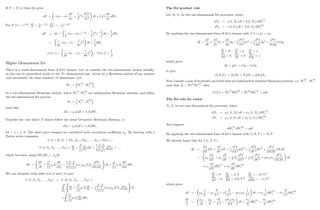
145. Another common form is
d
X
Y
=
X
Y
dX
X
dY
Y
dXdY
XY
+
dY
Y
2
!
As an example suppose we have
dS1 = 0:1dt + 0:2dW
(1)
t ;
dS2 = 0:05dt + 0:1dW
(2)
t ;
= 0:4
d
S1
S2
= X
1
Y Y
X
Y 2
+ 2
Y
X
Y 3 X Y
1
Y 2
dt + X
1
Y
dW
(1)
t Y
X
Y 2
dW
(2)
t
where
X = 0:1; Y = 0:05
X = 0:2; Y = 0:1
d
S1
S2
=
0:1
S2
0:05
S1
S2
2
+ 0:01
S1
S3
2
0:008
1
S2
2
dt + 0:2
1
S2
dW
(1)
t 0:1
S1
S2
2
dW
(2)
t
Producing Standardized Normal Random Variables
Consider the RAND() function in Excel that produces a uniformly distributed random number over 0 and
1; written Unif[0;1]: We can show that for a large number N,
lim
N!1
r
12
N
N
P
1
U (0; 1) N
2
N (0; 1) :
Introduce Ui to denote a uniformly distributed random variable over [0; 1] and sum up. Recall that
E [Ui] = 1
2
V [Ui] = 1
12
The mean is then
E
N
P
i=1
Ui = N=2
so subtract o¤ N=2; so we examine the variance of
N
P
1
Ui
N
2
V
N
P
1
Ui
N
2
=
N
P
1
V [Ui]
= N=12
As the variance is not 1, write
V
N
P
1
Ui
N
2
for some 2 R: Hence 2 N
12
= 1 which gives =
p
12=N which normalises the variance. Then we achieve
the result r
12
N
N
P
1
Ui
N
2
:
39
Rewrite as
N
P
1
Ui N 1
2
q
1
12
p
N
:
and for N ! 1 by the Central Limit Theorem we get N (0; 1).
Generating Correlated Normal Variables
Consider two uncorrelated standard Normal variables 1 and 2 from which we wish to form a correlated
pair 1; 2 ( N (0; 1)), such that E [ 1 2] = : The following scheme can be used
1. E [1] = E [2] = 0 ; E [2
1] = E [2
2] = 1 and E [12] = 0 (* 1; 2 are uncorrelated) :
2. Set 1 = 1 and 2 = 1 + 2 (i.e. a linear combination).
3. Now
E [ 1 2] = = E [1 ( 1 + 2)]
E [1 ( 1 + 2)] =
E 2
1 + E [12] = ! =
E 2
2 = 1 = E ( 1 + 2)2
= E 2
2
1 + 2
2
2 + 2 12
= 2
E 2
1 + 2
E 2
2 + 2 E [12] = 1
2
+ 2
= 1 ! =
p
1 2
4. This gives 1 = 1 and 2 = 1+
p
1 2 2 which are correlated standardized Normal variables.
40

146. 1
M
MA
AT
TE
EM
MÁ
ÁT
TI
IC
CA
A D
DI
IS
SC
CR
RE
ET
TA
A
Índice
Unidad 1: Lógica y teoría de conjuntos....................................................................................................... 2
1. Definiciones ......................................................................................................................................... 2
2. Leyes de la lógica ............................................................................................................................... 2
3. Reglas de inferencia........................................................................................................................... 3
4. Lógica de predicados......................................................................................................................... 3
5. Teoría de conjuntos............................................................................................................................ 3
Unidad 2: Inducción matemática.................................................................................................................. 4
1. Métodos para demostrar la verdad de una implicación................................................................ 4
2. Inducción matemática ........................................................................................................................ 4
Unidad 3: Relaciones de recurrencia........................................................................................................... 4
1. Ecuaciones de recurrencia homogéneas........................................................................................ 5
2. Ecuaciones de recurrencia no homogéneas .................................................................................. 5
3. Sucesiones importantes..................................................................................................................... 5
Unidad 4: Relaciones..................................................................................................................................... 6
1. Definiciones ......................................................................................................................................... 6
2. Propiedades de las relaciones.......................................................................................................... 6
3. Matriz de una relación........................................................................................................................ 6
4. Relaciones de equivalencia y de orden........................................................................................... 6
5. Elementos particulares....................................................................................................................... 7
Unidad 5: Álgebras de Boole ........................................................................................................................ 7
1. Definiciones y axiomas ...................................................................................................................... 7
2. Funciones booleanas ......................................................................................................................... 8
3. Propiedades de los átomos............................................................................................................... 9
4. Mapa de Karnaugh............................................................................................................................. 9
5. Isomorfismos entre álgebras de Boole.......................................................................................... 10
Unidad 6: Teoría de grafos.......................................................................................................................... 10
1. Definiciones de grafos y digrafos ................................................................................................... 10
2. Aristas, vértices, caminos y grafos................................................................................................. 10
3. Grafos de Euler................................................................................................................................. 12
5. Representación de grafos por matrices ........................................................................................ 13
6. Niveles................................................................................................................................................ 14
7. Algoritmos de camino mínimo......................................................................................................... 14
Unidad 7: Árboles ......................................................................................................................................... 15
1. Definiciones ....................................................................................................................................... 15
2. Árboles generadores........................................................................................................................ 16
3. Algoritmos para hallar un árbol generador mínimo ..................................................................... 16
Unidad 8: Redes de transporte................................................................................................................... 16
1. Definiciones ....................................................................................................................................... 16
2. Algoritmo de Ford-Foulkerson ........................................................................................................ 17
2
Unidad 1: Lógica y teoría de conjuntos
1. Definiciones
Lógica: estudio de las formas correctas de pensar o razonar.
Proposición: afirmación que es verdadera o falsa, pero no ambas.
Proposición primitiva: proposición que no se puede descomponer en otras dos o más proposiciones.
Siempre son afirmativas.
Proposición compuesta: proposición formada por dos o más proposiciones relacionadas mediante
conectivas lógicas.
Tablas de verdad:
p q p
(NOT)
p q
(AND)
p q
(OR)
p q
(XOR)
p  q
(IF)
p  q
(IIF)
p  q
(NOR)
p | q
(NAND)
V V F V V F V V F F
V F F F V V F F F V
F V V F V V V F F V
F F V F F F V V V V
Nota: proposiciones  líneas de tabla.
Negación: no, nunca, jamás, no es cierto que.
Conjunción: y, e, pero, como, aunque, sin embargo, mientras.
Disyunción: o, a menos que.
Disyunción excluyente: o bien.
Implicación: cuando, siempre que.
Doble implicación: si y sólo si (sii), cuando y solo cuando.
{|} y {} son los únicos conjuntos adecuados de un solo conectivo diádico.
“p q” “p q”
 Si p, entonces q.
 p implica q.
 p solo si q.
 p es el antecedente, q es el consecuente.
 q es necesario para p.
 p es suficiente para q.
 p es necesario y suficiente para q.
 p si y solo si q.
Tautología: proposición que es verdadera siempre.
Contradicción: proposición que es falsa siempre.
Contingencia: proposición que puede ser verdadera o falsa, dependiendo de los valores de las
proposiciones que la componen.
2. Leyes de la lógica
1) Ley de la doble negación p  p
2) Ley de conmutatividad a) p  q  q  p
b) p  q  q  p
3) Ley de asociatividad a) p  (q  r)  (p  q)  r
 p  q  p  q
 p  q  (p  q)  (q  p)
 (p  q)  (p  q)  (p  q)
 a  (b  c)  (a  b)  (a  c)
 (p  q)  t  (p  t)  (q  t)

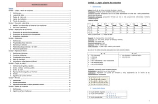
147. 3
b) p  (q  r)  (p  q)  r
4) Ley de distributividad a) p  (q  r)  (p  q)  (p  r)
c) p  (q  r)  (p  q)  (p  r)
5) Ley de idempotencia a) p  p  p
b) p  p  p
6) Ley del elemento neutro a) p  F0  p
b) p  T0  p
7) Leyes de De Morgan a) (p  q)  p  q
b) (p  q)  p  q
8) Ley del inverso a) p  p  T0
b) p  p  F0
9) Ley de dominancia a) p  T0  T0
b) p  F0  F0
10)Ley de absorción a) p  (p  q)  p
b) p  (p  q)  p
Dual de S: Sea S una proposición. Si S no contiene conectivas lógicas distintas de  y  entonces el dual de
S (S
d
), se obtiene de reemplazar en S todos los  () por  () y todas las T0 (F0) por F0 (T0).
Sean s y t dos proposiciones tales que s  t, entonces s
d
 t
d
.
 Recíproca: (q  p) es la recíproca de (p  q)
 Contra-recíproca: (q  p) es la contra-recíproca de (p  q)
 Inversa: (p  q) es la inversa de (p  q)
3. Reglas de inferencia
Modus ponens o Modus ponendo ponens
p  q
p
 q
Modus tollens o Modus tollendo tollens
p  q
q
 p
4. Lógica de predicados
Función proposicional: expresión que contiene una o más variables que al ser sustituidas por elementos del
universo dan origen a una proposición.
Universo: Son las ciertas opciones “permisibles” que podré reemplazar por la variable.
Cuantificador universal: proposición que es verdadera para todos los valores de en el universo.
Cuantificador existencial: proposición en que existe un elemento del universo tal que la función
proposicional es verdadera.
5. Teoría de conjuntos
Conjunto de partes: dado un conjunto A, p(A) es el conjunto formado por todos los subconjuntos de A,
incluídos A y . Si A tiene elementos, p(A) tendrá elementos. Ejemplo:
Negación de proposiciones cuantificadas:
 [x p(x)]  x p(x)
 [x p(x)]  x p(x)
 x [p(x)  q(x)]  x p(x)  x q(x)
 x [p(x)  q(x)]  x p(x)  x q(x)
 x [p(x)  q(x)]  x p(x)  x q(x)
 x p(x)  x q(x)  x [p(x)  q(x)]
 x [p(x)  q(x)] ≠ x p(x)  q(x)
4
Pertenencia: un elemento “pertenece” a un conjunto.
Inclusión: un conjunto está “incluido” en un conjunto.
Operaciones entre conjuntos:
Unión:
Intersección:
Diferencia:
Diferencia simétrica:
Complemento:
Leyes del álgebra de conjuntos: Para cualquier A, B  U:
Leyes conmutativas
Leyes asociativas
Leyes distributivas
Leyes de idempotencia
Leyes de identidad
Complementación doble
Leyes del complemento
Leyes de De Morgan
Unidad 2: Inducción matemática
1. Métodos para demostrar la verdad de una implicación
1) Método directo: V  V
2) Método indirecto:
a) Por el contrarrecíproco: F  F
b) Por el absurdo: supongo el antecedente verdadero y el consecuente falso y busco llegar a una
contradicción de proposiciones.
2. Inducción matemática
I)
II) 
Unidad 3: Relaciones de recurrencia
Orden de una relación: mayor subíndice – menor subíndice.
 

148. 5
1. Ecuaciones de recurrencia homogéneas
Sea la ecuación (*). Resolverla significa:
I) Hallar las raíces de la ecuación característica de (*):
II) Utilizar los teoremas siguientes para hallar la solución.
Teorema 1: si y son soluciones de la ecuación (*), entonces también es solución de (*)
.
Teorema 2: si es raíz de la ecuación característica, entonces es solución de (*).
Teorema 3: si y ( ) son soluciones de la ecuación característica, entonces es
solución de (*)y
Teorema 4: si es raíz doble de la ecuación característica, entonces es solución de (*).
Teorema 5: si es raíz doble de la ecuación característica, entonces es solución
de (*) y
2. Ecuaciones de recurrencia no homogéneas
Sea la ecuación (*), con . Resolverla significa:
I) Resolver la ecuación homogénea asociada y obtener .
II) Hallar una solución particular de la ecuación (*), .
III) La solución general será:
Nota: en la solución particular propuesta no debe haber sumandos que aparecen en la solución de la
ecuación homogénea.
propuesta
(a no es raíz de la ecuación
característica)
(a es raíz de multiplicidad t de la
ecuación característica)
Polinomio de grado k y 1 no es raíz de la
ecuación característica
Polinomio genérico de grado k
Polinomio de grado k y 1 es raíz de
multiplicidad t de la ecuación característica
Polinomio genérico de grado k
multiplicado por
ó
Caso especial 1:
I) Proponer una solución para
II) Proponer una solución para
III) La solución será .
Caso especial 2:
I) Proponer una solución para
II) Proponer una solución para
III) La solución será . Luego, comparar con la solución del homogéneo y arreglar si es
necesario.
3. Sucesiones importantes
Interés Fibonacci Torres de Hanoi Desarreglos
an = 1,12.an-1 Fn = Fn-1 + Fn-2 hn = 2hn-1 + 1 dn = (n – 1).(dn-1 + dn-2)
6
Unidad 4: Relaciones
1. Definiciones
Producto cartesiano:
Relación n-aria: dado un conjunto A se llama relación R en conjunto A R  AA. Una relación se puede
definir por extensión (mencionando todos sus elementos) o por comprensión (dando una característica de
los elementos).
Relación „R‟: Siendo x A, y A, decimos que xRy (x,y) R.
Relación inversa: dada , la relación inversa es tal que:
2. Propiedades de las relaciones
Sea R una relación en el conjunto A.
1) R es reflexiva  x A: xRx
2) R es simétrica  x,y A : (xRy  yRx)
3) R es transitiva  x,y,z A : (xRy  yRz)  xRz
4) R es antisimétrica  x,y A : (xRy  yRx  x=y)
Nota: Todo elemento cumple las tres primeras consigo mismo. Cuidado con la 4º: no simétrica 
antisimétrica.
3. Matriz de una relación
Sea R una relación en un conjunto finito A. La misma puede representarse matricialmente por:
siendo n=|A| definida por
Relación de orden entre matrices booleanas: . Es decir, una matriz C es
menor a D si D tiene al menos los mismos 1 en las mismas posiciones que C.
Sea I la matriz identidad de n x n. Entonces:
 R es reflexiva
 R es simétrica
 R es antisimétrica (el producto se entiende posición por posición)
 R es transitiva
4. Relaciones de equivalencia y de orden
Relación de equivalencia (~) Relación de orden ( )
- Reflexividad
- Simetría
- Transitividad
- Reflexividad
- Antisimetría
- Transitividad
 Orden total:  x,y A : (xRy  yRx). En el diagrama de Hasse se ve una línea recta.
 Orden parcial: x,y A : (xRy  yRx)
(Si no es orden total, es orden parcial.)
Repaso de funciones
Sean A y B dos conjuntos. Una relación es función si:
a A / f(a) = b0 f(a) = b1 (b0, b1 B b0  b1) (No existe elemento del dominio que tenga dos imágenes)
Sea  función, a A, b B:
 f es inyectiva  a1  a2  f(a1)  f(a2) (Para puntos distintos del dominio, distintas imágenes)
 f es sobreyectiva   b B,  a A / f(a) = b (La imagen de A es todo B)
 f es biyectiva  f es inyectiva y sobreyectiva (Si es biyectiva existe la inversa)

149. 7
Clase de equivalencia: sea R una relación de equivalencia en A. Se llama clase de equivalencia de un ,
al conjunto
Teorema: sea R una relación de equivalencia en A. Se verifica:





Conjunto cociente: . El conjunto cociente es una partición de A.
Partición: es una partición del conjunto A si y solo si:
1)
2)
3)
4)
Congruencia módulo n: En , y para , se define la relación
Diagrama de Hasse: representación gráfica simplificada de un conjunto (finito) ordenado parcialmente. Con
ellos se eliminan los lazos de reflexividad y los atajos de transitividad. Si dos elementos están relacionados,
digamos aRb, entonces dibujamos b a un nivel superior de a.
Ejemplo: sea el conjunto A = {1, 2, 3, 4, 5, 6, 10, 12, 15, 20, 30, 60} (todos los divisores de 60). Este
conjunto está ordenado parcialmente por la relación de divisibilidad. Su diagrama de Hasse puede ser
representado como sigue.
5. Elementos particulares
Sea R una relación de orden en A:
Maximal: x0 es maximal de A x A : x0Rx (x0 no se relaciona con nadie).
Minimal: x0 es minimal de A x A : xRx0 (No hay elementos que se relacionen con el x0.)
Sea X un subconjunto de A:
Cota Superior: x0 A es Cota Superior de X x X : xRx0.
Cota Inferior: x0 A es Cota Inferior de X x X : x0Rx.
Supremo: s A es el Supremo de X s es la menor de todas los cotas superiores x X : xRs.
Ínfimo: i A es Ínfimo de X i es la mayor de todas las cotas inferiores x X : iRx.
Máximo: M A es Máximo de X M es supremo de X y M X.
Mínimo: m A es Mínimo de X m es ínfimo de X y m X.
Unidad 5: Álgebras de Boole
1. Definiciones y axiomas
8
Álgebra de Boole: Sea K ( ) un conjunto no vacío que contiene dos elementos especiales, 0 (cero o
elemento neutro) y 1 (uno o elemento unidad) sobre el cual definimos las operaciones cerradas +,  y el
complemento. Entonces =(K, 0, 1, +, , ) es un Álgebra de Boole si cumple las siguientes condiciones:
A1) Axioma de conmutatividad x + y = y + x
x.y = y.x
A2) Axioma de asociatividad (x + y) + z = x + (y + z) = x + y + z
(x.y).z = x.(y.z) = x.y.z
A3) Axioma de la doble distributividad x.(y + z) = x.y + x.z
x + (y.z) = (x + y).(x + z)
A4) Axioma de existencia de elementos neutros x + 0 = x
x.1 = x
A5) Axioma de existencia de complementos x + = 1
x. = 0
Expresión dual: se obtiene cambiando todos los +() por  (+) y los 0(1) por 1(0).
Principio de dualidad: en toda álgebra de Boole, si una expresión es válida, su expresión dual también lo es.
1) Ley del doble complemento: = x
2) Leyes de Morgan: a) = .
b) = +
3) Leyes conmutativas: a) x + y = y + x
b) x.y = y.x
4) Leyes asociativas: a) x + (y + z) = (x + y) + z
b) x.(y.z) = (x.y).z
5) Leyes distributivas: a) x + (y.z) = (x + y).(x + z)
b) x.(y + z) = xy + xz
6) Leyes de idempotencia: a) x + x = x
b) x.x = x
7) Leyes de identidad: a) x + 0 = x
b) x.1 = x
8) Leyes de inversos: a) x + x = 1
b) x.x = 0
9) Leyes de acotación: a) x + 1= 1
b) x.0 = 0
10) Leyes de absorción: a) x + xy = x x + xy = x + y
b) x.(x + y) = x x.(x + y) = x.y
Permitido Prohibido
 x + y = 0  (x = 0)  (y = 0)
 x.y = 1  (x = 1)  (y = 1)
 x + y = z + y  x + y = z + y  x = z
 x + y = x.y  x = y
 x.y = 0  (x = 0) (y = 0)
 x + y = y + z  x = z
2. Funciones booleanas
Función booleana: . Dadas n variables, existen funciones
booleanas posibles.
Observación:
    
  +  
PROBLEMA
TABLA EXPRESIÓN de f
EXPRESIÓN
SIMPLIFICADA
CIRCUITO

150. 9
“0”
MINITERMINOS MAXITERMINOS
m = x.y.z M = x + y + z
Forma canónica, normal, normal disyuntiva SP:
suma booleana de minitérminos.
Forma canónica, normal, normal conjuntiva PS:
producto booleano de maxitérminos.
f(x,y,z)  suma de los minitérminos que dan 1 f(x,y,z)  producto de los maxitérminos que dan 0
Codificación: x  1, x  0 Codificación: x  0, x  1
Orden en un álgebra de Boole: sea = (K,+, ,0,1,-) un álgebra de Boole. En K se define:
a b aRb a b a b a a b b a b
Teorema: . Todo álgebra de Boole está acotada.
Átomo de un álgebra de Boole: x x es un átomo de B
y B: (y  x y = 0 y = x )
Nota: Si B tiene n átomos  B tiene 2
n
elementos.
Circuitos lógicos:
3. Propiedades de los átomos
1) x átomo  (El producto de cualquier elemento de B con un átomo es 0
o es el átomo)
2) x0, x1 átomos distintos  x0.x1 = 0 (Si hay dos átomos distintos el producto entre ellos es 0)
3) Sean átomos de B  (Si hay un x que multiplicado
por cada uno de los átomos da 0, x es el 0)
Teorema: sean los átomos de B. Entonces tales que
.
Teorema: , con átomo de B.
Nota: Si n es la cantidad de variables de f, el número máximo de términos es 2
n
.
4. Mapa de Karnaugh
Para simplificar una función booleana. Se colorean los cuadrados de los minitérminos correspondientes y
luego se escribe cada término, teniendo en cuenta que si un cuadrado tiene un vecino (abajo, arriba,
derecha o izquierda) este último no se escribe.
xyzw 00 01 11 10
00 0 1 3 2
01 4 5 7 6
11 12 13 15 14
10 8 9 11 10
f =  m(1, 3, 9, 11, 14, 6)
f = (w. + z. .y)
(simplificada)
Observación:
La suma de los minitérminos de una función producto de los maxitérminos que no aparecen en la SP.
 m(0, 1, 3, 5, 7) =  M(2, 4, 6)
10
5. Isomorfismos entre álgebras de Boole
Isomorfismo entre dos álgebras de Boole: sean B1 = (K1, +1, 1, 01, 11, 1) y B2 = (K2, +2, 2, 02, 12, 2) dos
álgebras de Boole. Se dice que B1 y B2 (#B1 = #B2) son isomorfos   biyectiva tal que:
El número de isomorfismos posibles es (#B1)!
Propiedades:
1) f(01) = 02
2) f(11) = 12
3) f(átomo B1) = átomo B2
4) x R1 y  f(x) R2 f(y)
Unidad 6: Teoría de grafos
1. Definiciones de grafos y digrafos
Grafo no orientado: terna G = (V,A,) que representa una relación entre un conjunto finito de Vértices (
) y otro conjunto finito de Aristas (A), y  es la función de incidencia.
: A  X(V), siendo X(V) = {X: X  V |X|= 1 o 2}.
Si (a) = {u,v} entonces
u y v son extremos de a
u y v son v rtices adyacentes
a es incidente en u y v
Grafo orientado / digrafo: terna D = {V,A,) con que representa una relación entre un conjunto finito
de Vértices y otro conjunto finito de Aristas, y  es la función de incidencia.
: A  V x V.
Si (a) = (v,w) entonces
v es extremo inicial y w es extremo final de a
v y w son v rtices adyacentes
a incide positivamente en w y negativamente en v
2. Aristas, vértices, caminos y grafos
Aristas
Aristas adyacentes: aristas que tienen un solo extremo en común.
Arista paralelas o múltiples: a a son aristas paralelas  a  a . Es decir, sii  no es inyectiva.
Lazo o bucle: arista que une un vértice con sí mismo.
Arista incidente: Se dice que “e es incidente en v” si v esta en uno de los vértices de la arista e.
Extremo (para digrafos): Un extremo es inicial(final) si es el primer(ultimo) vértice de la arista.
Aristas paralelas (para digrafos): Si E.I(a) = E.I(b)  E.F(a) = E.F(b) en otro caso son anti paralelas.
Puente: Es la arista que al sacarla el grafo deja de ser conexo.
Vértices
Vértices adyacentes: Se dice que “v y w son adyacentes” si existe una arista entre los dos vértices.
 Un vértice es adyacente a sí mismo si tiene lazo.
Grado de un vértice: gr(v) es la cantidad de aristas que inciden en él. Los lazos cuentan doble.
 Se dice que un vértice es „par‟ o „impar‟ según lo sea su grado.
 gr v
v
 La cantidad de vértices de grado impar es un número par.
 Si gr(v) = 0, v es un vértice aislado.
Grado positvo (para digrafos): gr v es la cantidad de veces que se usa el vértice como extremo final.
Grado negativo (para digrafos): gr v es la cantidad de veces que se usa el vértice como extremo inicial.

151. 11
Nota: Si v V gr(v)  2  el grafo tiene un circuito.
 gr v gr v
 grtotal(v) = gr v gr v
 grneto(v) = gr v gr v
 El lazo cuenta como arista incidente positiva y negativamente en el vértice.
Vértice de aristas múltiples: Es aquel que tiene más de un arista.
Caminos
Camino: sucesión finita no vacía de aristas distintas que contengan a vx y vy en su primer y último término.
Así: {vx,v1},{v2,v3},...,{vn,vy}
Longitud del camino: número de aristas de un camino.
Circuito o camino cerrado: camino en el cual v vn.
Camino simple: camino que no repite vértices.
 v w v w camino de v a w camino simple de v a w
Circuito simple: circuito que no repite vértices salvo el primer y último vértice.
Ciclo: circuito simple que no repite aristas.
 Circuito simple de longitud  3 en grafos ( 2 en digrafos) es un ciclo.
Grafos
Orden de un grafo: Es su número de vértices.
Grafo acíclico: grafo que no tiene ciclos.
Grafo conexo: grafo tal que dados 2 vértices distintos es posible encontrar un camino entre ellos.
camino de a )
Grafo simple: grafo que carece de aristas paralelas y lazos.
Grafo regular: Aquel con el mismo grado en todos los vértices.
Grafo k-regular: G=(V,A, ) es k-regular v gr v k
Grafo bipartito: Es aquel con cuyos vértices pueden formarse dos conjuntos disjuntos de modo que no haya
adyacencias entre vértices pertenecientes al mismo conjunto.
Grafo Kn,m: grafo bipartito simple con la mayor cantidad de aristas.
 # n
= n.m
Grafo Kn: grafo simple con n vértices y la mayor cantidad de aristas.
 # n
=
n n
Grafo completo: grafo simple con mayor cantidad de aristas. Todos están conectados con todos.
 v V, gr(v) = #V – 1.
 Si G(V,A) es completo  G es regular (No vale la recíproca)
 Dos grafos completos con mismo #V son isomorfos.
Grafo complemento: dado G=(VG,AG) simple se llama grafo complemento a tal que
. Es el grafo G‟ que tiene conectados los vértices no conectados de G y desconectados los
vértices conectados de G.
 G  G‟ = Grafo completo.
 Si dos grafos son complementarios, sus isomorfos también.
 Sea grG v k  grG
v – k –
v1
v2
v3
v5
v4
v1 v1
v2 v3
v4 v5
v5
v3
v2
v4
G G’
12
Grafo plano: Aquel que admite una representación bidimensional sin que se crucen sus aristas.
Grafo ponderado: Es el grafo en cual cada arista tiene asignado un n° real positivo llamado peso.
Digrafo: Grafo con todas sus aristas dirigidas. Por tanto, los pares de vértices que definen las aristas, son
pares ordenados.
Digrafo conexo: Si su grafo asociado es conexo.
Digrafo fuertemente conexo: v V  camino que me permite llegar a cualquier otro vértice.
Digrafo k-regular: D=(V,A, ) es k-regular v gr v gr v k
Subgrafo de G: Dado G = ( , ), G‟ = ( ‟, ‟) es subgrafo de G si ‟ V y ‟  A
Grafo parcial de G: Dado G = ( , ), G‟ = ( ‟, ‟) es grafo parcial de G si ‟ V y ‟  A
Multigrafo: Grafo que tiene alguna arista múltiple.
 Un multigrafo se transforma en grafo añadiendo un vértice en mitad de cada arista múltiple.
Pseudografo: Grafo con algún lazo.
3. Grafos de Euler
Grafo de Euler: grafo en el cual se puede encontrar un ciclo o un camino de Euler.
 Camino de Euler: camino que no repite aristas.
 Circuito de Euler: circuito que no repite aristas.
Teorema de Euler:
 Para grafos conexos:
 G tiene un Camino de Euler  G tiene exactamente 2 vértices de grado impar.
 G tiene un Circuito de Euler  G tiene exactamente 0 vértices de grado impar.
 Para digrafos:
 G tiene un Camino de Euler   u,w V (u  w)
gr u gr u
gr w gr w
gr v gr v v
 G tiene un Circuito de Euler  v V gr v gr v
Grafo de Hamilton: grafo en el cual es posible hallar un camino o circuito de Hamilton.
 Camino de Hamilton: Es un camino que no repite vértices. (Puede no pasar por todas las aristas)
 Circuito de Hamilton: Es un circuito que no repite vértices. (Puede no pasar por todas las aristas)
Teorema de Ore: Si un grafo es conexo con y    G es Grafo
Hamiltoniano.
Teorema de Dirac: un grafo simple con es Hamiltoniano si
4. Isomorfismos de grafos
Dados G=( , ) y G‟=( ‟, ‟), se denomina isomorfismo de G a G’ a la aplicación biyectiva f tal que para a,b
V, {a,b} A  se cumple {f(a),f(b)} ‟. Es decir, la aplicación que relaciona biyectivamente pares de
vértices de A con pares de vértices de ‟, de modo que los v rtices conectados siguen estándolo.
 # = # ‟ y # = # ‟
 Se cumple que (a)=(f(a))
 Si dos grafos son isomorfos, sus complementarios también.
 G y G‟ tienen igual cantidad de vértices aislados.
 G y G‟ tienen igual cantidad de lazos o bucles.
 Se mantienen los caminos.
 Se mantienen los ciclos.
 Si dos grafos complementarios son isomorfos se los llama auto complementarios.

152. 13
 Dos grafos simples G1 y G2 son isomorfos  para cierto orden de sus vértices las MA son iguales.
Automorfismo: Es un isomorfismo en sí mismo. f(a) = a.
5. Representación de grafos por matrices
Grafos Digrafos
Matriz de
adyacencia
( ) tal que: con
cantidad de aristas con extremos
y
 Matriz simétrica.
 gr(vi) = aij + 2.aii (i  j)
( ) tal que con
cantidad de aristas con E.I en vi y E.F en
vj
 No necesariamente simétrica.
Matriz de
incidencia
( ) tal que
, con
( ) tal que
, con
Propiedad: en la matriz G k
, cada coeficiente aij indica la cantidad de caminos de longitud k que hay
entre vi y vj.
Matriz de conexión: Dados G=(V,A, ) con y . Se define la siguiente relación:
.
Matriz de adyacencia booleana: sea un grafo G=(V,A, ) con v vn y a am . Se define la
matriz de adyacencia de G a una matriz booleana de tal que:
a3
v3 v4
a4
a1
v1 v2
v5
a6
a5
a2
v1 v2 v3 v4 v5
v1 0 1 1 0 0
v2 1 1 0 1 0
v3 1 0 0 2 0
v4 0 1 2 0 0
v5 0 0 0 0 0
gr(v1)
gr(v1)
v4
v2
a4
a6
a5
a3
a1
v1
v3
a2
a1 a2 a3 a4 a5 a6
v1 1 0 0 0 0 1
v2 1 2 1 0 0 0
v3 0 0 0 1 1 1
v4 0 0 1 1 1 0
v5 0 0 0 0 0 0
gr(v1)
| |
2
v1 v2 v3 v4 v5
v1 0 0 1 0 0
v2 1 1 0 0 0
v3 0 0 0 1 0
v4 0 1 1 0 0
v5 0 0 0 0 0
a1 a2 a3 a4 a5 a6
v1 1 0 0 0 0 -1
v2 -1 1 1 0 0 0
v3 0 0 0 -1 -1 1
v4 0 0 -1 1 1 0
v5 0 0 0 0 0 0
| |
0
gr+
(v1)=aij,(aij0)
gr -
(v1)=aij,(aij0)
14
G mij tal que mij
si vi es adyacente a vj
si vi es adyacente a vj
Matriz de incidencia booleana: sea un grafo G=(V,A, ) con v vn y a am . Se define la
matriz de adyacencia de G a una matriz booleana de tal que:
G mij tal que mij
si ai es incidente a vj
si ai es incidente a vj
6. Niveles
Vértice alcanzable: sea D=(V,A) un digrafo. Se dice que se alcanza de camino dirigido de
a .
Niveles de un digrafo: Un conjunto vértices N constituye o está en nivel superior a otro conjunto de vértices
K si ningún vértice de N es alcanzable desde algún vértice de K.
Dibujar MA
i = 1
while MA:
Nivel i = vi’s tales que sus filas y columnas en MA sean nulas
MA = MA – {columnas y filas que sean nulas}
i = i + 1
Nivel 1: A,G
Nivel 2: B
Nivel 3: E
Nivel 4: C
Nivel 5: F
Nivel 6: D
7. Algoritmos de camino mínimo
Objetivo: Hallar el camino mínimo de S a L:
 (v) es la etiqueta del vértice v.
 i es un contador.
Algoritmo de Moore o BFS (Breadth First Search)
 Dado un grafo o digrafo no ponderado, calcula la distancia entre dos vértices.
(S) = 0
i = 0
while (vértices adyacentes a los etiquetados con i no etiquetados):
(v) = i+1
if (L is etiquetado): break
i = i+1
Algoritmo de Dijkstra
 Dado un grafo o digrafo con pesos no negativos, calcula caminos mínimos del vértice a todos los
vértices.
(S) = 0
for v in V:
(v) = 
T = V
C
D
F
B
G
A
E
A
B C D
E F G
Solo flechas
descendentes!

153. 15
while (L T):
Elijo v T con mínimo (v) adyacente al último etiquetado
x / x adyacente v:
(x) = min{(x), (v) + a(v,x)}
T = T – {v}
Algoritmo de Ford
 Solo para digrafos, acepta pesos negativos y detecta circuitos negativos.
(S) = 0
for v in V:
(v) = 
j = 1
while ( j ≠ |V|):
T ={v V / v sea adyacente al último etiquetado}
x V, v T :
(v) = min{(x), (v) + a(v,x)}
Si no hubo cambios: break
Else: j = j + 1
return T
Unidad 7: Árboles
1. Definiciones
Árbol: G=(V,A) es un árbol   u,v V (u v  ! camino simple de u a v)
Teorema 1: dado un grafo G=(V,A). Las siguientes afirmaciones son equivalentes:
a) G es conexo y acíclico
b) G es acíclico y si se le agrega una artista deja de serlo
c) G es conexo y si se le elimina una arista deja de serlo
d) G es árbol
Teorema 2: dado un grafo G=(V,A). Las siguientes afirmaciones son equivalentes:
a) G es conexo y acíclico
b) G es conexo y
c) G es acíclico y
Propiedad: si G es un árbol con  hay al menos 2 vértices de grado 1.
Bosque: un grafo G=(V,A) es bosque  G es acíclico.
 Los bosques son grafos no conexos cuyas componentes conexas son árboles.
 t, siendo t la cantidad de árboles del bosque.
Arboles con raíz: G=(V,A) digrafo conexo es un árbol con raíz 
Hoja / terminal: Vértice sin hijos.
Vértice interno: Vértice con hijos.
Árbol n-ario: todos los nodos tienen a lo sumo n hijos.
Árbol n-ario completo: todos los nodos tienen 0 o n hijos.
Nivel de un vértice: número de aristas que le separan de la raíz. La raíz tiene nivel 0.
Altura de un árbol: máximo nivel de sus vértices.
Árbol equilibrado: las hojas llegan al mismo nivel.
16
Teorema: Si T = (V, A) es una árbol m-ario completo con i vértices internos entonces:
2. Árboles generadores
Árbol generador: T=( , ) es un árbol generador de G=( , ) 
T es árbol
T G
T G
Árbol generador minimal: es un árbol generador, de peso mínimo. No es único.
Teorema: G es un grafo no dirigido y conexo  G tiene árbol generador.
3. Algoritmos para hallar un árbol generador mínimo
Sea G = (V, A) un grafo conexo ponderado. Existen dos algoritmos para hallar un árbol generador mínimo
de G.
Algoritmo de Prim
v = vértice cualquiera de G
T = {v}
while (|T| ≠ |V|):
a = arista de mínimo peso incidente en un v T y un w  T
T = T + {w}
return T
Algoritmo de Kruskal
a = arista de mínimo peso de G
T = {a}
while (|T| |V|-1):
b = arista de mínimo peso tal que b  T y T + {b} es acíclico
T = T + {b}
return T
Unidad 8: Redes de transporte
1. Definiciones
Red de transporte: sea G = (V, A) un digrafo conexo y sin lazos. G es una red de transporte si se verifican:
1) Vértice Fuente: ! vértice f V / gr f (no llegan flechas)
2) Vértice Sumidero: ! vértice s V / gr s (no salen fleches)
3) Capacidad de la Arista:  una función  / si a = (vi, vj) A, C(a) = Cij
Flujo de una red: Si G = (V, A) es una red de transporte se llama flujo de G a una función F: A  N0 tal que:
1) a A: F(a)  C(a) (Si F(a) = C(a) se dice que la arista está saturada)
2) v V (v  f , v  s) se tiene que (Flujo entrante = Flujo saliente)

154. 17
Teorema 1: Si F es el flujo asociado a una red de transporte se cumple que
(Todo lo que sale de la fuente llega al sumidero)
Valor del flujo: suma de los flujos de todas las aristas que salen del vértice fuente:
Corte de una red: Un corte (P, ) en una red de transporte G = (V, A) es un conjunto P tal que:
f s
Capacidad de un corte: Se llama capacidad de un corte (P, ) al número: Es la
suma de todas las aristas incidentes en v y w tal que v P y w . (Las aristas por donde pasa el corte).
Teorema 2: Sea F un flujo de la red G = (V, A) y sea (P, ) un corte de G. Entonces: C(P, )  val(F)
Teorema 3 (del flujo Máximo y Corte Minimal): Si C(P, ) = val(F)  el flujo es máximo y el corte es
minimal.
Teorema 4: C(P, ) = val(F) 
2. Algoritmo de Ford-Foulkerson
Se utiliza para hallar el flujo máximo en una red de transporte.
Dada una red de transporte G = (V, A), con f (fuente) y s (sumidero):
 (v) función de etiquetación de v.
 ek capacidad residual de vk.
1) Poner en la red un flujo compatible.
2) Etiqueto la fuente con – 
3) Para cualquier vértice x adyacente a a, etiquetamos a x:
a) Si , etiquetamos x con ).
b) Si , no etiquetamos x.
4) Mientras exista (x a) en V tal que x esté etiquetado y exista una arista (x,y) tal que y no esté
etiquetado, etiquetamos a y:
a) Si , etiquetamos y como min
b) Si , no etiquetamos y.
5) Mientras exista (x a) en V tal que x esté etiquetado y exista una arista (x,y) tal que y no esté
etiquetado, etiquetamos a y:
c) Si , etiquetamos y como min
d) Si , no etiquetamos y.
F = 0
saturada
P