Downloaded 128 times
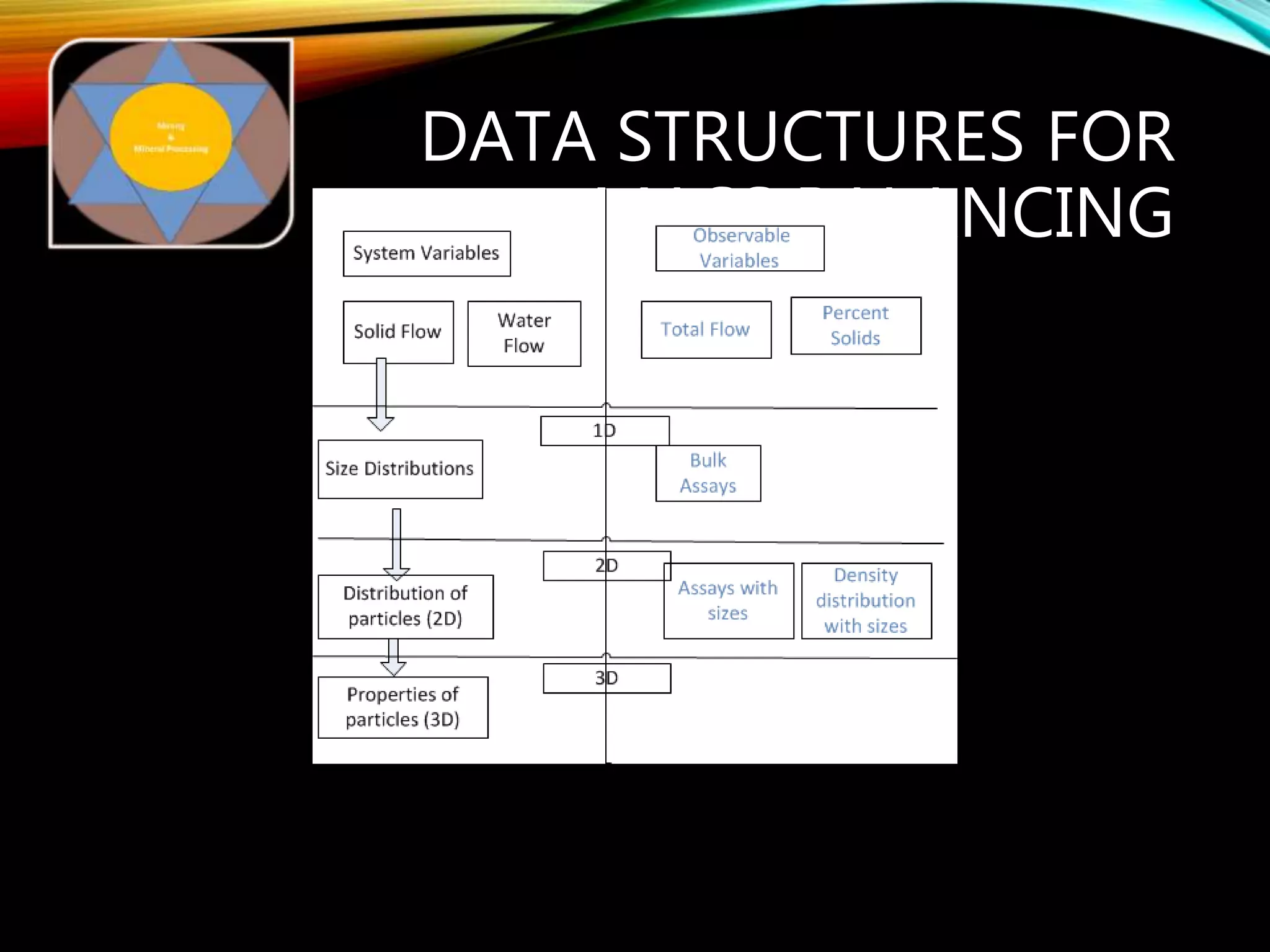


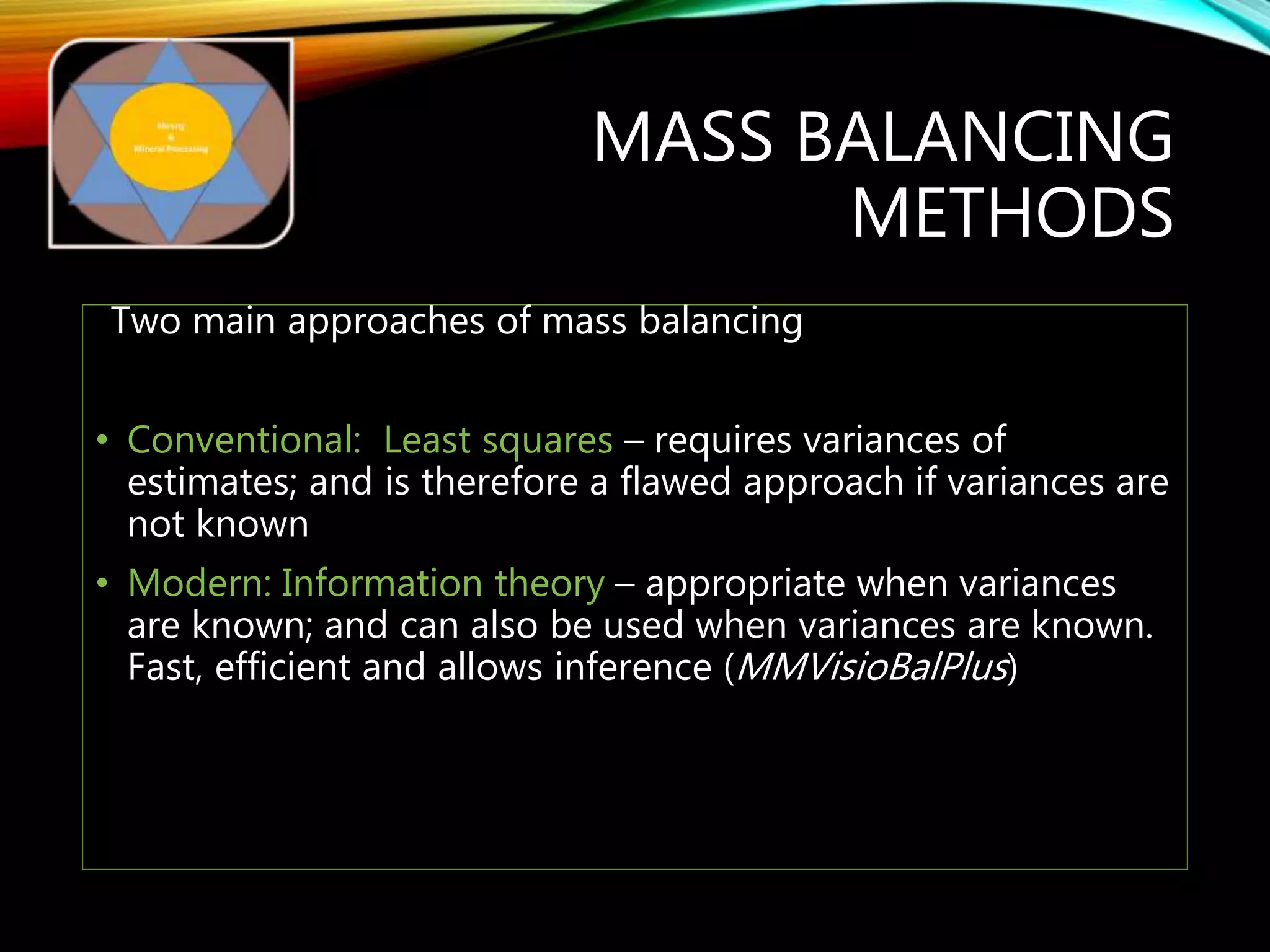
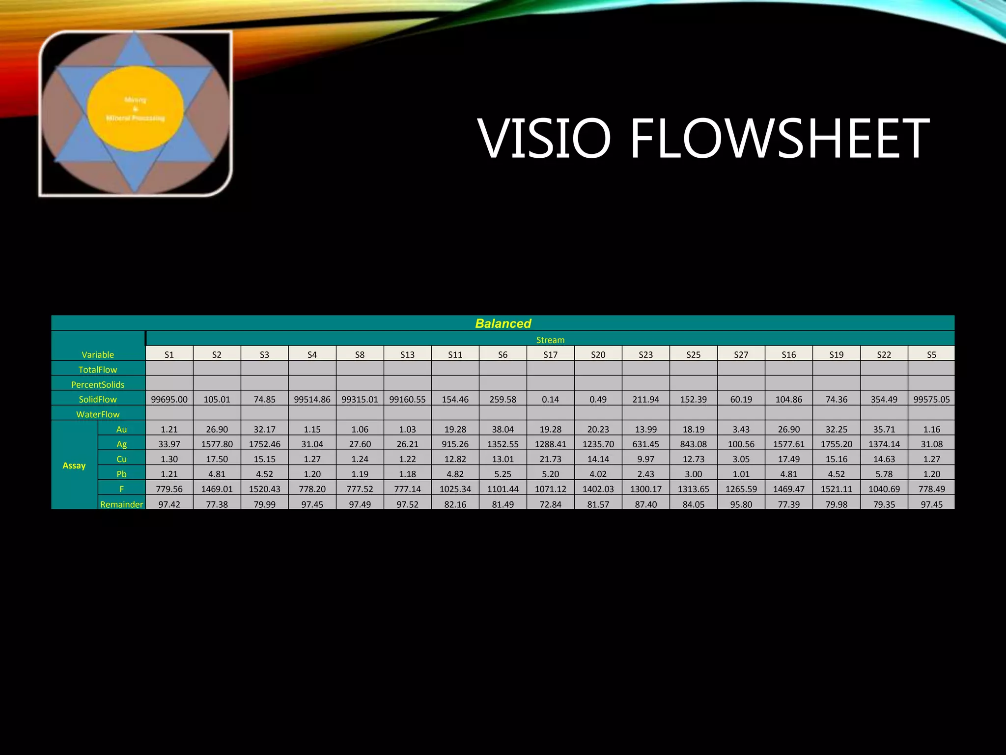
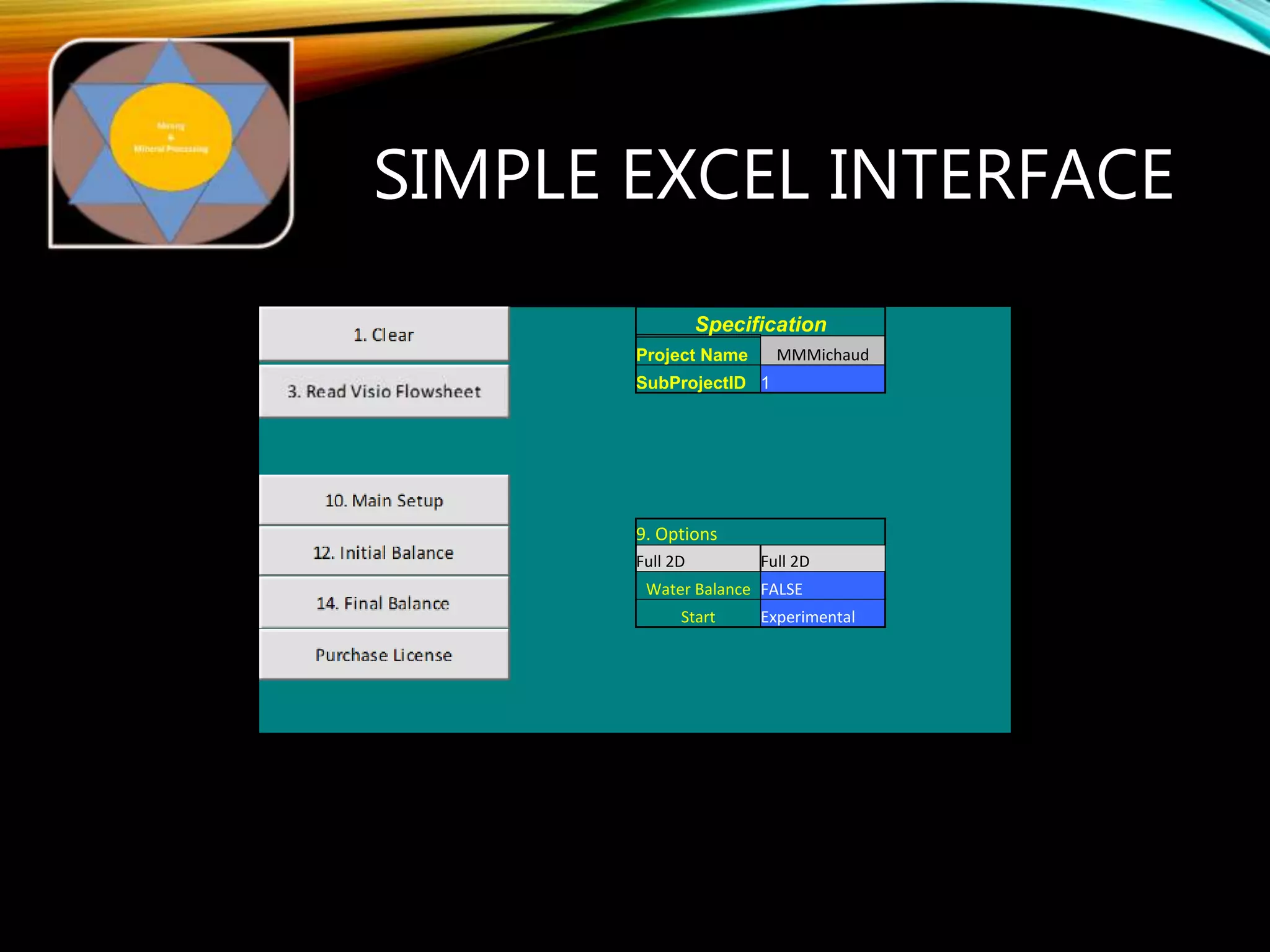
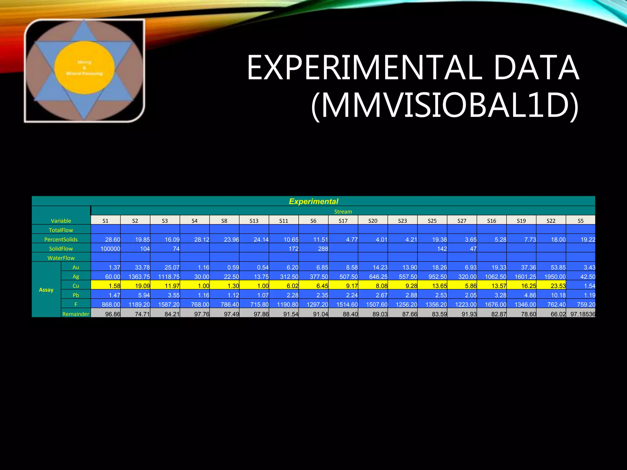
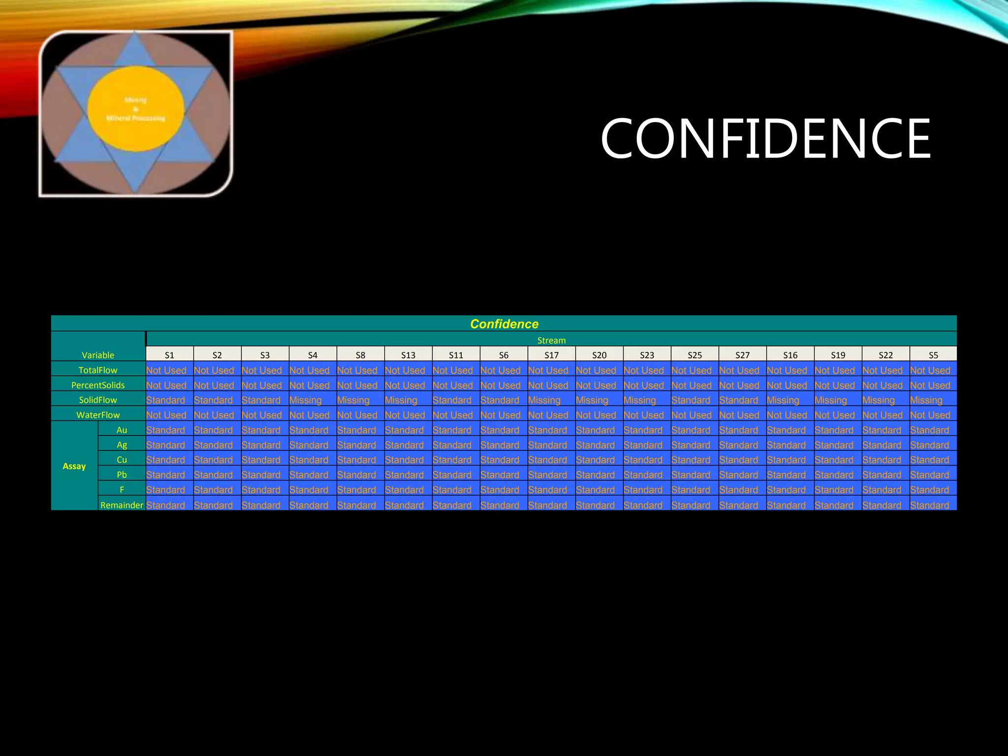
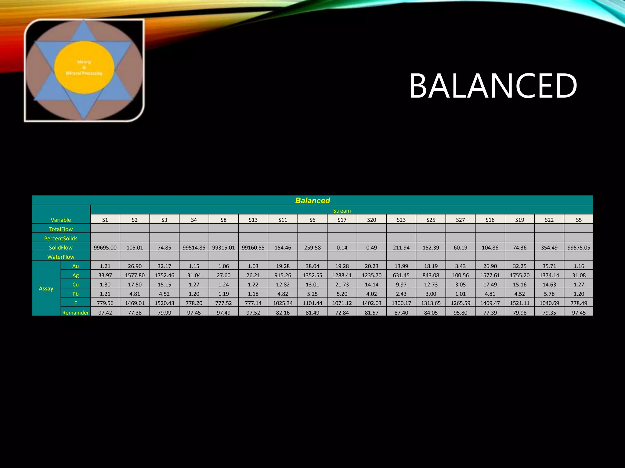

The document outlines the Midas approach to mass balancing in metallurgical accounting, emphasizing the importance of understanding particle behavior through detailed mass balances at various levels (0D, 1D, 2D, 3D) for accurate simulation. It discusses the benefits of recognizing multimineral particles, optimizing flotation efficiency, and using advanced simulation methods to improve operational performance, potentially saving millions per plant. Several software systems from Midas Tech for mass balance analysis are also introduced, promoting a modern approach using information theory.


