MartinDickThesis

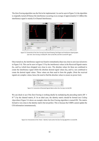
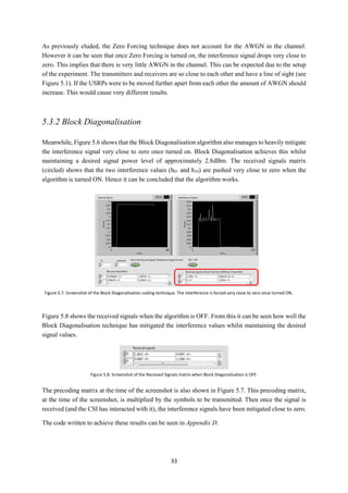
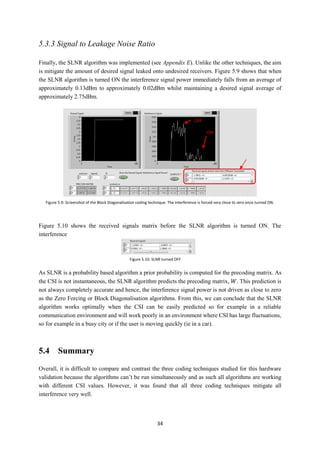
Comparison of Coding Techniques
Used to Mitigate Multi-User
Interference in MU-MIMO Systems
Martin Dick
April 2015
ck
April 2015
Final year project thesis submitted in support of the degree of
Master of Engineering in Electronic & Communications
Department of Electrical & Electronic Engineering
University of Bristol

i
DECLARATION AND DISCLAIMER
Unless otherwise acknowledged, the content of this thesis is the original work of the author. None
of the work in this thesis has been submitted by the author in support of an application for another
degree or qualification at this or any other university or institute of learning.
The views in this document are those of the author and do not in any way represent those of the
University.
The author confirms that the printed copy and electronic version of this thesis are identical.
Signed:
Dated:

ii
Abstract
As wireless technologies advance towards 5G cellular networks, the proliferation of devices
sharing the fixed spectrum and demanding ever higher data rates continues to accelerate.
Predictions suggest that by 2025 there will be a “10,000-fold increase in data traffic
demand”[1]
. It is obvious that current networks will be unable to handle this. A huge capacity
jump is required and fast. MIMO1
technology can provide the capacity jump required to fulfil
this proposed Multi-User (MU) telecoms bottleneck.
MIMO antennas technology uses multiple transmit and receive antennas to utilise spatial
diversity in the channel, this enables the transmitted data to use the same time and frequency
slots. Thus a substantial increase in spectral efficiency (bits/s/Hz) can be obtainable. However,
the reuse of frequency at each transmitter has been found to create a major problem called co-
channel interference.
Solutions to this can be found using Interference Alignment techniques, more specifically
Linear Precoding. Four Linear Precoding techniques: Zero Forcing, Block Diagonalisation,
Minimum Mean Square Error and Signal to Leakage Noise Ratio have been analysed. A
MATLAB simulation model was created and the Bit Error Rate performance of each algorithm
measured. The algorithms were first compared against themselves (different user numbers) and
then against each other.
To support the research, hardware was used to validate the initial conclusions drawn from the
software. USRPs2
and LabVIEW software were used to recreate a real-world propagation
environment where the algorithms were implemented and tested.
It has been found that all coding techniques bring significant reductions in co-channel
interference. However, some address the effects of AWGN3
in the channel more effectively
than others. MMSE4
and SLNR’s5
error rate performance was found to be the best due to
them both removing the AWGN noise effect coupled with the use of diversity. This is
especially true as the number of mobile users is increased.
1
Multiple Input, Multiple Output
2
Software defined radios
3
Thermal noise in the channel caused by nature
4
Minimum Mean Square Error algorithm
5
Signal to Leakage Noise Ratio algorithm

iii
Acknowledgements
The author wishes to thank the following for their contributions of time, support and guidance:
To Prof. Mark Beach for his invaluable guidance and support.
To Mr. Yue Tian for his patience, professionalism and friendship.
To Mr. Ben Lavasani and National Instrument’s for providing training in LabVIEW software
at the beginning of the year.

iv
List of Abbreviations and Symbols
Acronyms
4G Fourth Generation
5G Fifth Generation
AWGN Additive White Gaussian Noise
BD Block Diagonalisation
BER Bit Error Rate
BPSK Binary Phase Shift Keying
BS Base Station
CCI Co-Channel Interference
CSI Channel State Information
FDD Frequency Division Duplex
FDMA Frequency Division Multiple Access
IA Interference Alignment
IoT Internet of Things
LTE Long Term Evolution
LTE-A Long Term Evolution Advanced
MIMO Multiple Input, Multiple Output
MISO Multiple Input, Single Output
MMSE Minimum Mean Square Error
MU Multi-User
MUI Multi User Interference
NI National Instruments
OFDM Orthogonal Frequency Division Multiplexing
QAM Quadrature Amplitude Modulation
QPSK Quadrature Phase Shift Keying
Rx Receiver
SLNR Signal to Leakage Noise Ratio
SNR Signal to Noise Ratio
SVD Singular Value Decomposition
TDD Time Division Duplex
TDMA Time Division Multiple Access
Tx Transmitter
USRP Universal Software Radio Peripheral
ZF Zero Forcing

v
Roman & Greek
𝐴 Complex amplitude of a signal
𝑒𝑎 Power (in Watts) of one Transmitter
𝐻 Channel
(. ) 𝐻 Hermitian
𝐼 Identity Matrix
𝐾 Number of Receivers communicating with BS
𝐿𝐼 Leakage Interference Power
𝑀 𝑇 Number of transmit antennas
𝑛 Noise (AWGN)
𝑛𝑢𝑚 Number of bits transmitted
𝑃 Transmit Power
𝑠 Symbols Transmitted
𝑇 Training Sequence
(. ) 𝑇 Transpose
𝑒 Exponential term
𝑗 Symbol used to denote complex number
𝜃 Beamforming degree angle
𝜎 Variance of the AWGN in the channel
𝛿 Normalisation factor to satisfy the power constraint

vi
Contents
Abstract...........................................................................................................................................................ii
Acknowledgements .......................................................................................................................................iii
List of Abbreviations and Symbols.................................................................................................................iv
Chapter 1 - Introduction ................................................................................................................................1
1.1 Motivation......................................................................................................................................1
1.2 Project Overview............................................................................................................................1
Chapter 2 - Background..................................................................................................................................3
2.1 Wireless Mobile Communication Basics.......................................................................................3
2.2 MIMO Systems..............................................................................................................................4
2.3 Channel State Information & Feedback.........................................................................................5
2.4 System Model ................................................................................................................................7
2.5 Co-Channel Interference................................................................................................................9
2.6 Interference Alignment ................................................................................................................10
2.7 Linear Precoding..........................................................................................................................10
Chapter 3 - Coding Algorithms.....................................................................................................................13
3.1 Overview......................................................................................................................................13
3.2 Zero Forcing.................................................................................................................................13
3.3 Block Diagonalisation..................................................................................................................15
3.4 Minimum Mean Square Error ......................................................................................................17
3.5 Signal to Leakage Noise Ratio.....................................................................................................18
Chapter 4 - Software Simulation .................................................................................................................21
4.1 Overview......................................................................................................................................21
4.2 Assumptions Made.......................................................................................................................22
4.3 Performance Comparison with Different User Numbers.............................................................23
4.4 Comparison of Algorithms...........................................................................................................26
Chapter 5 - Hardware Validation.................................................................................................................29
5.1 Overview......................................................................................................................................29
5.2 The Setup .....................................................................................................................................30
5.3 Results..........................................................................................................................................31
5.4 Summary......................................................................................................................................34

vii
Chapter 6 - Conclusions................................................................................................................................37
Chapter 7 - Further Work.............................................................................................................................39
7.1 Overview......................................................................................................................................39
7.2 Multiple Receive Antenna’s per User..........................................................................................39
7.3 Test with Better USRPs ...............................................................................................................39
7.4 Introduce More Channel Scenarios..............................................................................................40
Bibliography..................................................................................................................................................41
Appendix.......................................................................................................................................................43
Appendix A:..............................................................................................................................................43
Appendix B:..............................................................................................................................................44
Appendix C:..............................................................................................................................................45
Appendix D:..............................................................................................................................................45
Appendix E:..............................................................................................................................................45
Appendix F: ..............................................................................................................................................46
Appendix G:..............................................................................................................................................47

1
Chapter 1 - Introduction
1.1 Motivation
As wireless technologies and cellular networks advance from today’s 4G networks, the future beyond
LTE and LTE-A towards 5G remains uncertain. It is clear that the rapid consumption of wireless data
throughout the world continues to outpace the industry’s ability to meet demand. In fact it is forecast,
compared to current usage, that:
“In 2025 there will be a 10,000-fold increase in data traffic demand.” [1]
Contributing factors are: The availability and cost of connecting to the internet decreasing, the rapid
increase in the number of devices connecting to this internet, falling component costs and smart phone
penetration at an all-time high. Such an explosion in opportunity has given rise to the nascent Internet
of Things. The Internet of Things will induce everyday objects to get ‘online’, connecting to the internet
and exchanging data in real time 24 hours a day. Examples range from a coffee machine that turns on
when your alarm clock goes off, to a jet engine of an aeroplane that can notify engineers of a
malfunction, to a wearable device for monitoring health. Essentially: remote control, monitoring and
sensing will become possible for any device with an ON/OFF switch.
All of these devices use the radio spectrum to transmit and receive data. The small segment of this
spectrum reserved for telecommunications is saturated. Simon Saunders, Director of Technology at
Real Wireless has previously stated that due to the expected increase in devices:
“There's a significant risk of a spectrum crunch by 2020.” [2]
This problem has become known as the telecoms bottleneck. With the vast number of devices expected,
all demanding ever higher data rates within an already fixed spectrum, a huge capacity jump is required
and fast. MIMO technology can provide the required capacity jump by taking advantage of spatial
diversity through the use of multiple transmit and receive antennas. All of these transmitting antennas
work within the same time slots and frequency to increase substantially the spectral efficiency
(bits/s/Hz) possible.
1.2 Project Overview
The project has been split into three main parts:
1. To gain a thorough understanding of the Multi User (MU) coordination and cancellation
techniques and to then carefully choose the most applicable of these algorithms to research.
Also, to gain a general understanding of the LTE platform. This research is discussed in Chapter
2 – Background and Chapter 3 – Coding Algorithms.

2
2. To create a software simulation to understand, model and draw theoretical conclusions of these
coding algorithms in action. A MATLAB model was created and has been described in Chapter
4 – Software Simulation.
3. To validate these conclusions using hardware. This was achieved using National Instruments’
USRPs and LabVIEW software to simulate a real-world two by two MIMO open air channel
environment. The Set Up and Results of which have been discussed in Chapter 5 – Hardware
Validation.

3
Chapter 2 - Background
2.1 Wireless Mobile Communication Basics
Wireless mobile communication is the transmission of an analogue or digital information signal from a
‘Base-Station’ to a ‘Mobile User’. The ‘Mobile User’ can range from a mobile phone, to a laptop to a
coffee machine (see Motivation). In conventional wireless communications, a single antenna is used to
transmit data from a Base Station. This signal then passes through the ‘channel’ to a receiver antenna
at the mobile user. This channel is an open air environment with obstacles present such as buildings,
hills and even people.
Interference is the dominant limiting factor in the performance of today’s wireless networks.
Interference distorts the transmitted signal as it travels in the channel between transmit and receive
antennas. Typically, it refers to the superposition of unwanted signals [3].
Interference can be caused in multiple different ways. Two typical problems are: Rayleigh & Rician
Fading and AWGN noise.
A problem faced is Rayleigh Fading. When an electromagnetic field is met with obstructions such as
buildings, hills and people the wavefronts will be scattered and thus take many different paths
(multipaths) to reach the receive antenna. The resultant signal received is the sum of numerous
attenuated, reflected, transmitted and diffracted versions of the original signal. This creates a problem
called shadowing. As a result the average received signal power may be unreliable, prone to dropping
and subsequently may cause a reduction in data speed and an increase in the number of errors. These
multipaths also give rise to inter-symbol interference, where a symbol transmitted interferes with
subsequent symbols [4].
Rician Fading is similar to the Rayleigh Fading concept similarly utilising the summation of multipaths.
However, in Rician Fading a strong dominant signal is present. This dominant component is normally
a line-of-sight wave (no obstacles between base station and mobile user) and as such does not pose as
much of a problem.
Figure 2.1: A Base Station transmits to Mobile Users through the Channel. Arrows denote
the channel. (from A.Nix, 2014) [3]

4
Another difficulty to overcome is Additive White Gaussian Noise [5]. This is a thermal noise that affects
the transmitted signal when it propagates through the channel in the form of interference. It occurs due
to the effect of many random processes that occur in nature and presents a major problem in wireless
communication.
Mitigation of this interference and improvement in the reliability of data signals can be generated
through the use of diversity. Diversity can be achieved by means of two or more communication
channels with different characteristics. Therefore, there are a number of independent channels available
which can be exploited by the receiver. Thereby improving capacity and reliability.
In a wireless communication channel, there are three types of diversity characteristics which can be
successfully utilised:
1. Time Diversity – Retransmitting a signal after a suitable time delay using different time slots.
2. Frequency Diversity – Transmitting a signal on more than one frequency
3. Space Diversity – Using a number of different antenna spaced sufficiently apart to ensure
independent and uncorrelated fading.
Adopting one or all of these characteristics helps to stabilise a link between a transmitter and receiver
and as such improves performance by reducing the error rate. It must be noted that time and frequency
diversity are less desirable for mobile radio applications due to their requirement for extra signal
bandwidth.
The focus of this project, MIMO systems, take advantage of this spatial diversity.
2.2 MIMO Systems
As eluded to earlier, a single transmit and receive antenna gives rise to problems with multipath effects.
The use of two or more antennas can help mitigate these problems.
MIMO stands for Multiple Input, Multiple Output and is an antenna technology for wireless
communications. Multiple antennas are used at both the source (transmitter) and destination (receiver)
and utilises smart antenna technology. The main benefits of MIMO are transmission diversity and
spatial multiplexing. The same data can be transmitted from multiple antennas to create an improvement
in spatial diversity. This has been previously limited to only one transmit and one receive antenna
systems in order to satisfy processing power constraints needed. If the Mobile User is restricted to only
one receive antenna, the MIMO system becomes known as a MISO (Multiple Input, Single Output)
system.

5
Additionally, multiple different streams of data can be sent from each individual transmitter (spatial
multiplexing). This results in a multiplexing gain. This systematically improves the spectral efficiency
and capacity potential within a cell. Consequently, a huge increase in spectral efficiency (increase in
bits/s/Hz) is achieved. Whilst all the while minimising errors and optimising data speeds.
Over the last decade, this area of research has attracted a significant amount of interest [6]. At the
Mobile User, most user terminals can only support a single or very few number of antennas. This is due
to the small physical size and low cost requirement usually applicable within a device (for example in
a wearable fitness band). However, the Base Station can be equipped with a much larger number of
antennas. The more antennas the Base Station is equipped with, the more Degrees Of Freedom possible.
Degrees of Freedom is the number of independent channels exploited by the transmitter [7]. Therefore,
we get an improvement in spectral efficiency and hence more users can simultaneously communicate
with the Base Station in the same time-frequency resource.
2.3 Channel State Information & Feedback
The Channel State Information refers to the properties of the channel medium. This information
describes how a signal will propagate through the channel from transmitter to receiver. Therefore, it
represents the combined effect of fading, power decay, scattering and co-channel interference.
In MIMO systems where we have more than one transmitter and receiver, this CSI can be represented
as a channel matrix, H. The magnitude of each element within the matrix shows how much one signal
interacts with another.
Figure 2.2: General Outline of a MIMO System

6
So for example in Figure 2.3 in the above 2x2 MISO environment a channel matrix, 𝐻, representing the
CSI can be obtained:
𝑯 = [
𝒉 𝟎𝟎 𝒉 𝟎𝟏
𝒉 𝟏𝟎 𝒉 𝟏𝟏
] (2.1)
2x2 denotes the dimensions of the channel matrix (2 Transmit antennas, 2 Receive antennas). Each h
value represents the properties of the channel and can be represented in the form: 𝐴𝑒 𝑗𝜃
where 𝐴 equals
the complex amplitude and 𝜃 is equivalent to the beamforming degree at which the signal is transmitted
at.
In Figure 2.3, the desired signals are the green h00 and h11 values. The co-channel interference is
represented by the red h01 and h10 values. The elements of 𝐻 are assumed to be complex Gaussian
variables with zero-mean and unit variance.
In a real-world propagation environment, the CSI matrix is calculated at the receiver through the use of
a training sequence (or pilot sequence). A training sequence is a known signal transmitted and using the
combined knowledge of the transmitted and received signal, the channel matrix, 𝐻, can be calculated.
Let the training sequence, 𝑇, be denoted by: [T1,T2,…Tn] where the vector Ti is transmitted over the
channel as:
𝒓𝒊 = 𝑯. 𝑻𝒊 + 𝑨𝑾𝑮𝑵 (2.2)
Where received signal, yi, becomes: [y1,y2,…yn]. Therefore, using the knowledge of 𝑦 and 𝑃, the matrix
H can be calculated and fed back to the transmitter.
If the users are only separated by the spatial properties of the channel, accurate and timely Channel
State Information is imperative in order to achieve a high spatial multiplexing gain. Channel estimation
errors will degrade the performance of the system. Near perfect channel state information is a challenge,
especially in high mobility scenarios.
The assumption that full Channel State Information is available at the transmitter upon the time of
transmission is valid in time-division duplex (TDD) systems. This is because the uplink and downlink
channels are sharing the same frequency band. However, for frequency-division duplex (FDD) systems
Figure 2.3: Channel State Information in MISO systems

7
(see Figure 2.4), the CSI needs to be estimated at the receiver and fed back to the transmitter. This
creates time delays and as such the CSI is not instantaneous (see Further Work).
2.4 System Model
Figure 2.5 represents the general signal structure for LTE downlink and shows an outline of the general
steps in forming the transmitted downlink signal in the physical layer.
Throughout the project it is assumed that the transmitter (Base Station) has 𝑀 𝑇 antennas and serves 𝐾
receivers (users) within the same time slots and frequency. It is also assumed that the 𝐾th user receives
𝑆 𝐾 independent data streams [8].
From this, and using the knowledge of CSI gained in ‘Channel State Information and Feedback’ the
above transmission can be modelled as Equation 2.3 assuming a flat fading environment:
[
𝒓 𝟏
⋮
𝒓 𝑴
] = [
𝒉 𝟎𝟎 ⋯ 𝒉 𝟎𝑴
⋮ ⋱ ⋮
𝒉 𝑲𝟎 ⋯ 𝒉 𝑲𝑴
] [
𝒔 𝟏
⋮
𝒔 𝑴
] + [
𝒏 𝟏
⋮
𝒏 𝑴
] (2.3)
Figure 2.5: Block diagram of the signal structure for LTE in a typical MIMO environment (from Sesia, Toufik & Baker,
2009) [11]
Figure 2.4: Frequency Domain MISO System showing feedback of CSI data from User to Base Station
(Black arrow denotes feedback)
CSI Information
CSI Information

8
Equation 2.3 describes the system model for any MIMO transmission. 𝑟 𝑀 represents the received
symbols matrix and 𝑛 𝑀 represents the AWGN in the channel. 𝑛 represents all other noise that is not
detected by the channel matrix. Examples of these other sources of interference are things such as
jamming in military networks or self-interference created from nonlinearities in the radio frequency
components.
In the system model, the choice of an appropriate modulation and multiple-access technique for mobile
wireless data communications is critical to achieving good system performance. In LTE, QPSK and
QAM modulation schemes are used and OFDM is used as multiple-access technique.
2.4.1 Modulation Schemes – QPSK & QAM
In current LTE systems, data transmission uses different modulation methods: QPSK, 16 QAM and 64
QAM) as defined by the LTE scheduler depending on the scenario [9]. The higher the modulation
scheme, the more bits per symbol achievable and thus higher capacity. Therefore, 64QAM is the
preferred method because it achieves the highest capacity of six bits per symbol (see Motivation).
Quadrature Phase-Shift Keying (QPSK) modulates digital signals onto a radio-frequency carrier signal.
This is achieved using four phase states to code two digital bits shifted 45° from one another. Each
unique pair of bits generates a carrier with a different phase.
Quadrature Amplitude Modulation (QAM) uses both phase and amplitude variations of a carrier sine
wave. Here, two sine carriers are generated and mixed 90° out of phase with one another. Much greater
capacity can be achieved using QAM over PSK methods and as such, preferred [10].
The modulation scheme is selected depending on the current channel conditions and required data rate.
Figure 2.6: Constellation graphs of Modulation schemes used in LTE Systems (and the whole of this
project). The respective capacity of each is given above each graph [9]
Two Bits per Symbol Four Bits per Symbol Six Bits per Symbol

9
2.4.2 Multiple Access Methods - OFDM
Orthogonal Frequency-Division Multiplexing is used to separate data to be transmitted onto multiple
carrier frequencies and is an improvement upon traditional TDMA and FDMA multiple access methods.
By using several parallel data channels, a large number of closely spaced orthogonal sub-carrier signals
can be used to carry the data. The spacing between the sub-channels is such that they can be perfectly
separated at the receiver.
As Figure 2.7 shows, the non-frequency selective narrowband subchannels into which the frequency-
selective wideband channel is divided are overlapping but orthogonal with no need for guard-bands
[11].
The main advantages of OFDM are: High data capacity, high spectral efficiency, resilience to
interference, low-complexity receiver implementation. Therefore ideal for high data applications.
2.5 Co-Channel Interference
Co-Channel Interference is a type of interference that occurs due to the frequency reuse at all receivers.
It is caused by crosstalk between two or more radio transmitters operating on the same frequency and
presents a major problem for MIMO systems.
Because of this, signals propagating on the same channel and thus using the same frequency (co-channel
signals) arrive at the receiver from undesired transmitters at the base station as well as the intended
signal from within the cell.
This interference leads to a significant deterioration in MIMO performance unless it can be mitigated.
Obviously, this co-channel interference creates a large problem to MIMO systems. This is because all
transmitters spaced small distances apart are transmitting at the same frequency.
Receivers resistant to co-channel interference allow a dense geographical reuse of the spectrum and
thus a high capacity system. This can be achieved by using interference alignment techniques that take
Figure 2.7: Spectral Efficiency of OFDM: (a) classical multicarrier system spectrum; (b) OFDM
system spectrum. (from Sesia, Toufik & Baker, 2009) [11]

10
advantage of the structure of the co-channel interference. These techniques are designed to drive this
interference as close to zero as possible.
The most obvious approach to achieve this would be to consider only the strongest active co-channel
user signal at the receiver and to neglect all other active users as background noise. However, this
method has failed when tested in real-world propagation environments [12]. Consequently there has
been significant research into Interference Alignment, different way to mitigate the impact of co-
channel interference.
2.6 Interference Alignment
A simple and effective approach to mitigate all interference is to transmit signal orthogonally, in time
or frequency. However with the increasing demand expected (discussed in Motivation) more
sophisticated approaches are required. Interference Alignment (IA) is the most prominent new
approach. [13]
The idea of Interference Alignment is to coordinate the multiple transmitters present in MIMO systems
so that their mutual interference aligns at the receivers. It exploits the availability of multiple signalling
dimensions provided by multiple time slots, frequency blocks, or antennas. The transmitters jointly
design their transmitted signals in the multidimensional space so that when the signal inevitably arrives
at the unintended receiver, it is a null.
IA was first proposed in [14, 15]. It was found in [15] that the interference alignment strategy may
allow:
“The network’s sum data rate to grow linearly, and without bound, with the network’s size” [13]
This is an amazing solution to the Co-Channel interference problem and is in stark contrast with the
likes of FDMA and TDMA used in conventional wireless instances where the network’s sum data rate.
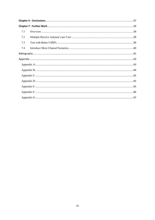
2.7 Linear Precoding
If the users are to be separated only by the spatial properties of the channel, the problem of co-channel
interference can be mitigated using linear precoding. This is the main premise of this project. Precoding
uses the Channel State Information at the transmitter to create a precoding matrix to mitigate this multi-
user interference.

11
Assuming we know the Channel State Information, the symbols to be transmitted can be multiplied by
this precoding matrix. Therefore, once the imperfect channel impacts on the transmitted symbols, the
received symbols at the receiver will have close to zero co-channel interference values. The point of
these coding techniques is to drive the interference values of h01 and h10 as close to zero as possible
whilst leaving the desired signal values h00 and h11 intact.
Using linear precoding, the transmitter multiplies the data symbol 𝑠 for each user 𝑘 by a precoding
matrix 𝑊𝑘 . Therefore the transmitted signal is a linear function: = ∑ 𝑊𝑘 𝑠 𝑘
𝐾
𝑘=1 . The resulting received
signal vector is [16]:
𝑦 𝑘 = 𝐻 𝑘 𝑊𝑘 𝑠 𝑘 + ∑ 𝐻 𝑘 𝑊𝑗 𝑠𝑗 + 𝑛 𝑘
𝑗 ≠𝑘
(2.4)
Where 𝑠 𝑘 denotes the 𝑘-th user transmit symbol vector, 𝐻 𝑘 denotes the channel matrix for the 𝑘-th user
and 𝑛 𝑘 denotes the AWGN in the channel
The second term in the above equation (∑ 𝐻 𝑘 𝑊𝑗 𝑠𝑗𝑗 ≠𝑘 ) represents the multi-user interference. The goal
of linear precoding is to design 𝑊𝑘 to drive this multi-user interference as close to zero as possible
based on the knowledge of the channel. There are a number of different ways to do this called, coding
algorithms. The main premise of the project is to investigate these algorithms, firstly theoretically, then
in hardware and to ultimately analyse them.
Tx–Symboltoantennamapping
Rx1Rx2
h00
h11
h10
h01
Bitstosymbolmapping-
QPSK
Precoding
b0,b1,b2,b3...
s0,s1,s2,s3...
s0,s2...
s1,s3...
r0,r2...
r1,r3...
DecodingDecoding
Figure 2.8: An example transmission model for Zero Forcing Precoding

13
Chapter 3 - Coding Algorithms
3.1 Overview
The coding algorithms associated with MIMO systems algorithms have drawn considerable during the
past decade. As such, many solutions have been proposed for the Co-Channel Interference problem.
The initial step for the project was to select the most appropriate Coding Algorithms to adopt.
The following were selected for in depth analysis:
 Zero Forcing
 Block Diagonalisation
 Minimum Mean Square Error (MMSE)
 Signal to Leakage Nosie Ratio (SLNR)
All algorithms selected work in the frequency domain and rely on perfect Channel State Information.
3.2 Zero Forcing
The Zero Forcing algorithm is the simplest precoding technique studied and as such has the lowest
computational complexity. Here, the multiuser interference is driven to zero. This is achieved by
projecting each data stream onto the orthogonal space of the co-channel interference. The precoding
matrix is simply an inversion of the channel matrix. This inverted channel matrix can then serve as a
weighting for the transmitting signal vector.
START
Generate bits to be transmitted.
All bits
transmitted?
Modulate bits into symbols. Bits
to Symbol mapping
Invert Channel Matrix, so that:
𝑊 = (𝐻 𝑇
)−1
Take transpose of Channel Matrix
to create HT
Multiply 𝑊 (precoding matrix) by
symbols
Transmit
FINISH
Figure 3.1: Flow Diagram of the Zero Forcing Process (see Appendix A)
YES
NO

14
Mathematically, the precoding matrix, W, is given by the Moore-Penrose pseudoinverse of H [17]:
𝑊 = 𝐇 𝐻
(𝐇𝐇 𝐻
)−1
(3.1)
Where, H is the channel between the Base Station and the Mobile Users and H is the Hermitian operator.
H is a K x M matrix with complex Gaussian distributed entries. The Hermitian operator is equivalent to
the conjugate transpose of the matrix. The conjugate transpose is used to preserve signal power as the
channel matrix values are complex. Furthermore, the transpose also ensures the precoding matrix is of
correct dimensions (𝑀 x 𝐾).
Therefore, when the inverse of the channel matrix (𝐇 𝐻
(𝐇𝐇 𝐻
)−1
) is multiplied by the channel (𝐇. 𝑊),
an identity matrix, 𝐼, is formed. This follows basic mathematics where any complex (or non-complex)
matrix, for example, 𝐴, is multiplied by its inverse, 𝐴−1
, the identity matrix is formed:
𝐴. 𝐴−1
= 𝐼 (3.2)
The identity matrix has the same dimensions as the channel matrix (K x M ). Therefore, when the
symbols (dimensions Kx1) are multiplied by the identity matrix, the symbols are returned exactly the
same. For example in a 2x2 channel matrix scenario where symbols: s0 and s1 are to be transmitted (a
more general case can be found in [16] and [18]):
[
𝑠0
𝑠1
][
1 0
0 1
] = [
𝑠0
𝑠1
] (3.3)
The interference is represented by the two zero values in the identity matrix. These interference values
have been ‘forced’ to ‘zero’ hence the algorithms name: ‘Zero Forcing’.
The transmitted signal is given by:
𝑥 = √ 𝑃𝑇
𝑊. 𝑠
√𝛿
(3.4)
Where, 𝑃𝑇 is the transmit power, 𝛿 is a normalisation factor used to satisfy the transmission power
constraint and 𝑥 is the received signal power [19]. The Zero Forcing algorithm ensures that the
interference is forced to zero. However, this is created at the cost of the received power for each user.
Upon transmission, the desired signal loses some power due to the precoding matrix, 𝑊.
Other factors which limit the viability of Zero Forcing methods is that complete knowledge of the
channel (full CSI) is required at the transmitter. Otherwise the algorithm performs sub-optimally [20]
Moreover, the complete nulling of the co-channel interference at the base station imposes the constraint
that the number of transmit antennas must be greater than or equal to the sum of all receive antennas
(𝑀 ≥ 𝐾). This condition is necessary in order to provide sufficient Degrees Of Freedom for the Zero
Forcing solution to force the CCI to zero at each user.
In summary, the major disadvantage of Zero Forcing is that it neglects the effect of AWGN in the
channel. Thus, theoretically, it will operate ineffectively under noise-limited scenarios (low SNR). This
shall be discussed in greater detail later in the project (see Software Simulation).

15
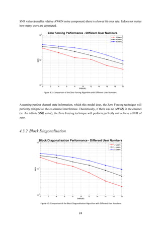
3.3 Block Diagonalisation
The Block Diagonalisation method is an improvement on the Zero Forcing method by increasing the
spatial diversity of each transmission. The symbols to be transmitted are combined and sent from all
transmitters. The Block Diagonalization process at the receiver then decodes the received signal to
cancel unwanted symbols and other interference at the receiver.
So for example in Figure 3.2, if the Base Station wants to send data symbols 𝑠0 to Rx1 and 𝑠1 to Rx2
both symbols will be combined and transmitted from both transmitters. Therefore, we have double the
amount of (useful) streams arriving at each receiver containing the wanted symbol. Hence an increase
in spatial diversity. The amount of (useful) streams arriving at the wanted receiver is equal to the amount
of transmit antennas. A decoding process is then needed at the receiver to separate these previously
combined symbols to get the correct symbols. So in our above example the 𝑠1 value is cancelled at Rx1
and the 𝑠0 value is cancelled at Rx2
The fundamental idea is to select a precoding matrix, 𝑊, so that: 𝑊. 𝐻 is exactly block diagonal. By
having a perfectly block diagonal matrix, all interference caused by other symbols and interference can
be perfectly cancelled. This can be achieved by choosing 𝑊 to be in the nullspace of each 𝐻 value (as
𝐻 changes for each aim user). 𝑊 can be found with unitary columns. All of this can be achieved using
the singular value decomposition of the channel matrix.
The main steps of the Block Diagonalisation precoding algorithm is two of these Singular Value
Decomposition (SVD) operations. The first precoding filter is used to completely eliminate the Multi-
User Interference (MUI) with noise. From this, the approximately parallel SU-MIMO channels are
obtained. The second precoding filter is implemented to parallelise each user’s streams. These two
filters are then combined to create the precoding matrix.
3.3.1 Singular Value Decomposition Function Explanation
The SVD function is a mathematical operation to factorise a real or complex matrix. It is closely related
to the eigendecomposition function [21]. For a factorisation of a complex matrix, 𝑀, the SVD operation
diagonalises the matrix chosen and returns three matrices:
Figure 3.2: Block Diagonalisation takes advantage of the spatial diversity of MIMO systems
𝑠0 + 𝑠1
𝑠0 + 𝑠1
𝑠0 + 𝑠1
𝑠0 + 𝑠1
𝑠1 𝑠1
𝑠0𝑠0

16
𝑀 = 𝑈Σ𝑉 𝑇
(3.5)
Σ - Diagonal matrix with the same dimensions as M with non-negative diagonal elements in decreasing
order. The diagonal entries are the non-negative square roots of the eigenvalues of 𝑀𝑀 𝑇
.
U – Numeric unitary eigenvectors matrix of 𝑀𝑀 𝑇
with dimensions: mxm.
V – Numeric unitary eigenvectors matrix of 𝑀 𝑇
𝑀 with dimensions: nxn. 𝑉 𝑇
is the Hermitian transpose
of 𝑀 (the complex conjugate of the transpose).
For the context of this project, in the scenario above, the complex matrix 𝑀 is the channel matrix 𝐻
containing the Channel State Information.
Assuming the channel state information is known perfectly, SVD precoding is known to achieve the
MIMO channel capacity [22].
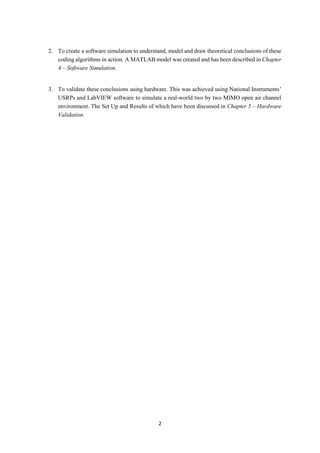
3.3.2 Method
We initially perform the SVD operation on the interference matrix: 𝐻̃𝑗. This interference matrix is a full
channel matrix for a MIMO system with the aim user (𝐻𝑗) disregarded (note no 𝐻𝑗 in the 𝐻̃𝑗 equation
below.
𝐻̃𝑗 = [𝐻1
𝑇
, … , 𝐻𝑗−1
𝑇
, 𝐻𝑗+1
𝑇
, … , 𝐻 𝐾
𝑇
] 𝑇
(3.6)
START
Create Interference Matrix, 𝐻𝑗
Performed for
all aim users?
Perform SVD function on 𝐻̃ to
find the Zero Space
Take the Left Hand Eigenvectors
of the ‘V’ values to create P1
Perform the SVD function on 𝐻𝑗 to
implement this zero space on the
interference (hence driving it to
null)
Create Aim User Matrix, 𝐻𝑗
Take the Left Hand Eigenvectors
of V again to create P2
𝑊 = 𝑃1 𝑃2
Multiply 𝑊 by symbols
Transmit
FINISH
NO
YES
Figure 3.3: Flowchart explaining the Block Diagonalisation process (see Appendix A)

17
The SVD operation already discussed can then be applied to the above interference channel matrix.
𝑆𝑉𝐷 𝑜𝑓 𝐻̃𝑗 = (𝑈̃ 𝑘
(1)
𝑈̃ 𝑘
(0)
) (
Σ 0
0 0
) (𝑉̃ 𝑘
(1)
𝑉̃𝑘
(0)
) (3.7)
In the above equation, the unitary matrix 𝑉̃ 𝑘
(1)
contains the first right eigenvectors. This is the
orthogonal basis in the 𝐻𝑗 zero space. This value is not good enough as a solution, this first SVD
operation finds the location of the zero space however we still have the interference values within this
matrix. 𝑉̃ 𝑘
(0)
is the last right eigenvectors. 𝑉̃ 𝑘
(1)
becomes the first precoding matrix, 𝑃1.
We then implement the SVD operation again on the aim user channel matrix, 𝐻𝑗 (the channel matrix
from the perspective of the aim user) multiplied by the first precoding matrix. We perform this to cancel
the interference within the channel.
𝑆𝑉𝐷 𝑜𝑓 𝐻𝑗. 𝑃1 = 𝑈𝑗 [
Σ𝑗 0
0 0
] [𝑉𝑗
(1)
𝑉𝑗
(0)
] (3.8)
The matrix 𝑉𝑗
(1)
then has no interference or noise associated with it and becomes our second precoding
matrix.
These two precoding matrices are multiplied together to create a final precoding matrix, 𝑊:
𝑊 = 𝑉𝑗
(1)
. 𝑉̃𝑘
(1)
= 𝑃1. 𝑃2 (3.9)
This process is then repeated for each aim user. See Appendix B for the implementation of the above
method.
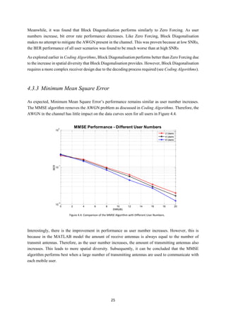
3.4 Minimum Mean Square Error
The Minimum Mean Square Error (MMSE) algorithm operates similarly to the Zero Forcing technique
by using a channel inversion. However, the MMSE method takes the AWGN into account and aims to
minimise the mean-square error between the estimate and the transmitted signal. Remember the Zero
Forcing method does not take this AWGN in the channel into account.
𝑊 = 𝐻 𝐻
(𝐻𝐻 𝐻
+
𝜎
𝑒𝑎
. 𝐼)
−1
(3.10)
The
𝜎
𝑒𝑎
. 𝐼 term accounts for the AWGN in the channel as a function of power. In the above equation,
𝑒𝑎 denotes the power (in Watts) of one transmitter and 𝜎 denotes the variance of the AWGN [23]. It
is equivalent to the combined power of all the transmitters divided by the signal to noise ratio of the
channel.
The algorithm also uses spatial diversity to improve reliability like Block Diagonalisation. Therefore,
theoretically, MMSE should outperform both Zero Forcing and Block Diagonalisation as it uses
diversity and accounts for the AWGN in the channel.

18
3.5 Signal to Leakage Noise Ratio
The Signal to Leakage Noise Ratio algorithm uses an alternative approach to the other three algorithms
studied [24]. Here, a new concept of signal leakage is considered. Leakage refers to the interference
caused by the signal intended for a desired user that is ‘leaked’ onto undesired users. This is an
inefficient waste of power as the leaked power just acts as interference upon undesired receivers. The
aim of the algorithm is to minimise this leaked power as close to zero as possible. Therefore, instead of
trying to perfectly cancel out the interference at each user (like for example Zero Forcing), SLNR
precoding chooses beamforming coefficients to maximise the Signal to Leakage Noise Ratio (SLNR)
for all users simultaneously.
Figure 3.4 shows a MIMO situation with three transmitting antennas and three users simultaneously
communicating with the Base Station. Similar to Block Diagonalisation and MMSE, all transmitters
communicate with each user. In each user scenario, the desired power (green arrow) will arrive at the
correct receiver, whilst some of the signal will be leaked onto other receivers (red arrows). These red
arrows create co-channel interference. The aim of the SLNR technique is to make the undesired red
arrow signal as small as possible, whilst making the green desired signal as large as possible.
This leakage proposition is in stark contrast to the previous three algorithms, where we have used the
signal to interference plus noise ratio (SINR) at the input of the receiver, given by:
𝑆𝐼𝑁𝑅𝑖 =
‖𝐻𝑖 𝑤𝑖‖2
𝑀𝑖 𝜎𝑖
2
+ ∑ ‖𝐻𝑖 𝑤 𝑘‖2𝐾
𝑘=1,𝑘≠𝑖
(3.11)
Where ‖𝐻𝑖 𝑤𝑖‖2
is equivalent to the power of the desired signal component for user 𝑖. At the same time,
part of this transmit power is leaked onto other receivers. Thus we can define a term for leakage power
attributed to user 𝑖:
∑ ‖𝐻 𝑘 𝑤𝑖‖2
𝐾
𝑘=1,𝑘≠𝑖
(3.12)
This is equivalent to:
𝐿𝐼 = ‖𝐻̃𝑖 𝑤𝑖‖
2
(3.13)
Figure 3.4: SLNR algorithm in practice on a 3x3 MIMO configuration. Green arrows denote desired signal and red indicate ‘leaked’ values.

19
Therefore we want this desired received signal power to be as large as possible compared to the leakage
power (hence a large ratio). These considerations can as such define an equation for the ratio, called the
Signal to Leakage Noise Ratio:
𝑆𝐿𝑁𝑅𝑖 =
‖𝐻𝑖 𝑤𝑖‖2
𝑀𝑖 𝜎𝑖
2
+ ‖𝐻̃𝑖 𝑤𝑖‖
2
(3.14)
Where 𝑀𝑖 = Number of Receive Antennas and 𝜎𝑖
2
= the variance of the AWGN. Here, the AWGN is a
random variable having an expected value equal to zero. A random variable’s power equals its mean-
squared value. The AWGN in this case has zero mean, therefore its power is equal to its variance.
Through this leakage idea, an optimisation problem can be created (similarly to the other three
algorithms) dealing with the total interfering power that user 𝑖 causes on all other users.
In contrast to the previous three algorithms, the SLNR solution does not require any dimension
condition on the number of transmit / receive antennas. It also takes the AWGN in the channel into
account, unlike the Zero Forcing algorithm and as such outperforms it.
‖𝐻1 𝑤1‖2
≈ 0
‖𝐻2 𝑤1‖2
‖𝐻 𝐾 𝑤1‖2
≈ 0
Figure 3.5: Example MISO system using the SLNR algorithm. Transmitter 2 transmits to User 2 but ‖𝐻 𝐾 𝑤1‖2
is leaked per extra K
users. We aim to minimise this leaked value as close to zero as possible.

21
Chapter 4 - Software Simulation
4.1 Overview
Three precoding algorithms were individually modelled using MATLAB, a numerical programming
software environment. This was used to create a model to simulate the bit error rate performance of the
algorithms in different theoretical scenarios. This could be achieved by changing different variables.
The algorithms could then be compared against themselves and subsequently against each other, to
draw theoretical conclusions on their overall performance.
START
Initialise: Number of Transmit and
Receive Antennas, SNR range,
Power per Transmitter, Number
of bits to transmit.
Generate Normalised Random
Channel Matrix, 𝐻.
Create Precoding Matrix &
Normalise.
Generate random QPSK symbol.
Multiply symbols by Precoding
matrix.
Add AWGN to create Received
Symbols.
Decoding (only necessary for
Block Diagonalisation).
Hard decision decoder to round
received symbols to closest QPSK
symbols.
Has a Bit Error
occurred?
Fill BER matrix
with a value 1.
Compare Sent Symbols and
Received Symbols.
Fill BER matrix
with a value 0.
Transmitted all
bits?
Iterate up to
next SNR value
Transmitted at
all SNR values?
Plot BER Graph
FINISH
Yes
Yes
Yes No
No
No
Key
Start / Finish Box
Process Box
Decision Box Figure 4.1: Flowchart explaining how the MATLAB simulation operated.

22
The flowchart above provides a description of how the MATLAB model worked. Two ‘for’ loops are
used. The first cycles through all SNR values which the amount of AWGN added to the transmitted
signal depends on. The second cycles through ‘𝑛𝑢𝑚’ times (𝑛𝑢𝑚 = number of bits transmitted) for the
chosen SNR value. The CSI is generated as a random K x M matrix (𝐾 = Number of Users, 𝑀 = Number
of Transmit Antennas).
A hard decision decoder was then modelled to compare the received symbols (including interference
and noise) to the transmitted symbols. If there was an error, ie. the received symbol did not equal the
transmitted symbol, a BER matrix would increase its value by one. This was done 𝑛𝑢𝑚 amount of times
per SNR value. The value of 𝑛𝑢𝑚 was increased up to 10,000 to ensure the results were accurate and
reliable. See Appendix A.
Note that upon each SNR iteration, each use of the channel corresponds to a new, independent matrix
for 𝐻.
The precoding techniques modelled were:
 Zero Forcing
 Minimum Mean Square Error
4.2 Assumptions Made
Due to the limitations of the project, a number of assumptions were made for the MATLAB model:
1. Bit Level Transmission - Transmissions was modelled at a bit level. Therefore, each individual
bit to be sent was precoded separately. In reality, transmission occurs at a packet level and so
each packet of bits is precoded.
2. Perfect Channel State Information – The coding algorithms chosen perform optimally under
this assumption. In reality, perfect CSI is difficult to achieve (see Further Research).
3. Zero Fading Channel – The model works in the frequency domain (not the time domain).
Therefore, memory in the channel has not been considered. The receiver does not take
multipaths into account (therefore no Rayleigh Fading considered). The first received symbol
is the only one considered this can be considered as a single dominant multipath and as such all
system components are memoryless. Time and Frequency diversity are not considered, only
spatial diversity. We model a line of sight propagation environment in free space. As such,
consider a perfect channel environment with only AWGN impacting upon the Signal to Noise
Ratio.
4. One Receive Antenna Per User – A MISO (multiple input, single output) model is assumed.
Multiple antennas are used at the Base Station (transmitter) and the destination (receiver) has
only one antenna. Therefore there are multiple users communicating with the base station but
each user has only one receive antenna.

23
5. QPSK modulation – The QPSK modulation scheme is used. Therefore, only four different bit
symbols can be transmitted.
6. Each Antenna normalised to unit average power – The power levels transmitted should be
similar. Therefore each receiver can effectively receive data from each transmitter. In reality,
if there is a power imbalance the mobile user will discard the low-power signal and only receive
the high-power data transmitted [25].
Further research of this project could be to expand upon this MATLAB model to improve upon all of
these assumptions.
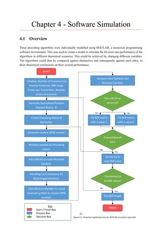
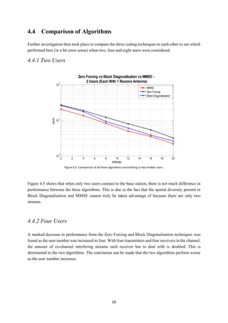
4.3 Performance Comparison with Different User Numbers
To begin with, the performance of the coding techniques were compared against themselves as user
number increased. For each selected algorithm, three different scenarios were tested based upon a
variant number of users. In this case the Base Station is transmitting to: 2, 4 and 8 users. The bit error
rate performance of each algorithm was tested.
In all graphs, a SNR range from zero to twenty has been used. This is the most applicable range to a
real world propagation environment. A logarithmic Bit Error Rate scale is also used. Therefore, it is
much easier to compare graphical results against each other. A Bit Error Rate value of one (100
) is
equivalent to all received symbols being incorrect, whilst a BER of zero (10−∞
) is equivalent to all
received symbols being correct.
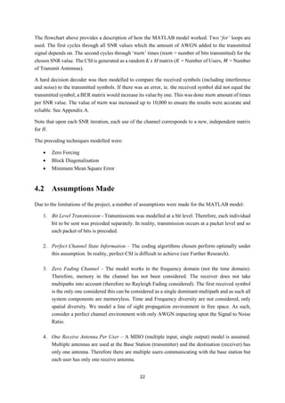
4.3.1 Zero Forcing
From Figure 4.2, it can be seen for Zero Forcing that as user number increases, the Bit Error Rate (BER)
performance gets worse.
This is an expected solution. This is because, the more users served by the Base Station, the more
interference the systems will suffer from. This interference is caused by more streams of co-channel
signals being received by each user. From this, the conclusion can be made that as the co-channel
interference increases the performance of Zero Forcing decreases.
As discussed in Coding Algorithms, the Zero Forcing technique does not account for the AWGN present
in the channel and only serves to mitigate the co-channel interference. This can be seen in Figure 4.2.
At low SNR values (larger relative AWGN noise component) there is a larger bit error rate than at high

24
SNR values (smaller relative AWGN noise component) there is a lower bit error rate. It does not matter
how many users are connected.
Assuming perfect channel state information, which this model does, the Zero Forcing technique will
perfectly mitigate all the co-channel interference. Theoretically, if there was no AWGN in the channel
(ie. An infinite SNR value), the Zero Forcing technique will perform perfectly and achieve a BER of
zero.
4.3.2 Block Diagonalisation
0 2 4 6 8 10 12 14 16 18 20
10
-2
10
-1
10
0
SNR(dB)
BER
Zero Forcing Performance - Different User Numbers
2 Users
4 Users
8 Users
Figure 4.2: Comparison of the Zero Forcing Algorithm with Different User Numbers.
0 2 4 6 8 10 12 14 16 18 20
10
-2
10
-1
10
0
SNR(dB)
BER
Block Diagonalisation Performance - Different User Numbers
2 Users
4 Users
8 Users
Figure 4.3: Comparison of the Block Diagonalisation Algorithm with Different User Numbers.

25
Meanwhile, it was found that Block Diagonalisation performs similarly to Zero Forcing. As user
numbers increase, bit error rate performance decreases. Like Zero Forcing, Block Diagonalisation
makes no attempt to mitigate the AWGN present in the channel. This was proven because at low SNRs,
the BER performance of all user scenarios was found to be much worse than at high SNRs
As explored earlier in Coding Algorithms, Block Diagonalisation performs better than Zero Forcing due
to the increase in spatial diversity that Block Diagonalisation provides. However, Block Diagonalisation
requires a more complex receiver design due to the decoding process required (see Coding Algorithms).
4.3.3 Minimum Mean Square Error
As expected, Minimum Mean Square Error’s performance remains similar as user number increases.
The MMSE algorithm removes the AWGN problem as discussed in Coding Algorithms. Therefore, the
AWGN in the channel has little impact on the data curves seen for all users in Figure 4.4.
Interestingly, there is the improvement in performance as user number increases. However, this is
because in the MATLAB model the amount of receive antennas is always equal to the number of
transmit antennas. Therefore, as the user number increases, the amount of transmitting antennas also
increases. This leads to more spatial diversity. Subsequently, it can be concluded that the MMSE
algorithm performs best when a large number of transmitting antennas are used to communicate with
each mobile user.
0 2 4 6 8 10 12 14 16 18 20
10
-2
10
-1
10
0
SNR(dB)
BER
MMSE Performance - Different User Numbers
2 Users
4 Users
8 Users
Figure 4.4: Comparison of the MMSE Algorithm with Different User Numbers.

26
4.4 Comparison of Algorithms
Further investigation then took place to compare the three coding techniques to each other to see which
performed best (in a bit error sense) when two, four and eight users were considered.
4.4.1 Two Users
Figure 4.5 shows that when only two users connect to the base station, there is not much difference in
performance between the three algorithms. This is due to the fact that the spatial diversity present in
Block Diagonalisation and MMSE cannot truly be taken advantage of because there are only two
streams.
4.4.2 Four Users
A marked decrease in performance from the Zero Forcing and Block Diagonalisation techniques was
found as the user number was increased to four. With four transmitters and four receivers in the channel,
the amount of co-channel interfering streams each receiver has to deal with is doubled. This is
detrimental to the two algorithms. The conclusion can be made that the two algorithms perform worse
as the user number increases.
0 2 4 6 8 10 12 14 16 18 20
10
-2
10
-1
10
0
SNR(dB)
BER
Zero Forcing vs Block Diagonalisation vs MMSE -
2 Users (Each With 1 Receive Antenna)
MMSE
Zero Forcing
Block Diagonalisation
Figure 4.5: Comparison of all three algorithms transmitting to two mobile users.

27
On the other hand, it was found that the MMSE algorithm actually increased in performance as the user
number was doubled. This was especially evident at high SNR values, compared to low SNR values,
where performance only slightly improved. This is evidenced by the slightly steeper curve.
4.4.3 Eight Users
When the model was tested for eight mobile users, a clear winner emerged - the MMSE algorithm. It
performed better than the Zero Forcing and Block Diagonalisation techniques especially at high SNR
values. As mentioned earlier, the MMSE algorithm removes the noise problem that is present in the
Zero Forcing and Block Diagonalisation algorithms. This, coupled with the increase in diversity
confirms the hypothesis that MMSE performs best in the MATLAB model scenario created.
0 2 4 6 8 10 12 14 16 18 20
10
-2
10
-1
10
0
SNR(dB)
BER
MMSE
Zero Forcing
Figure 4.6: Comparison of algorithms transmitting to four mobile users.

28
By numerically comparing the results at 20dB as in Table 4.1, we can see that the difference between
Zero Forcing and Block Diagonalisation is large. If one hundred bits were sent by the transmitter, on
average there will be 13 more bit errors by Zero Forcing and 9 more bit errors by Block Diagonalisation
compared to MMSE.
Zero Forcing Block Diagonalisation MMSE
Zero Forcing 0.04 0.13
Block Diagonalisation 0.04 0.09
MMSE 0.13 0.09
0 2 4 6 8 10 12 14 16 18 20
10
-2
10
-1
10
0
SNR(dB)
BER
MMSE
Zero Forcing
Table 4.1: Comparison of the difference in BER performance between each of the three algorithms at an SNR of 20dB
Figure 4.7: Comparison of all three algorithms transmitting to two mobile users.

29
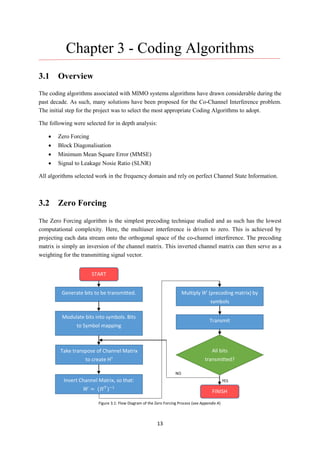
Chapter 5 - Hardware Validation
5.1 Overview
The final part of the project was to implement the coding algorithms into a real-world OFDM
propagation environment. Hardware could be used to create a real MIMO system to transmit real data
to independent receivers that represent the Mobile User. From this, the performance of the algorithms
could be tested upon real Multi User interference (CCI) as the CSI used would be real-life values.
Subsequently, the performance of all algorithms could be compared.
This was achieved using USRPs (Universal Software Radio Peripherals) provided by National
Instruments [26]. National Instruments (NI) is a producer of automated test equipment and virtual
instrumentation software based in Texas. Specifically, the ‘NI USRP-2920’ was used (see Figure 5.1).
The USRPs are a: “Tuneable RF transceiver” that works in a frequency range from “50MHz to 2.2GHz”
[27]. Put simply, they are software defined radios that can be used to recreate real world transmission
scenarios.
The USRPs work in conjunction with LabVIEW Software [28]. LabVIEW is a visual programming
language also designed by National Instruments. Together, using both the USRPs and LabVIEW code
provided by National Instruments, both single-channel and MIMO (multi-channel) wireless
communications systems can be prototyped.
A MIMO configuration could be created by connecting two USRPs together using a MIMO cable. Each
USRP contains one transmitter and one receiver. Therefore, the amount of them connected together
accounts for the size of MIMO configuration. For example, three USRPs connected would create a 3x3
MIMO propagation environment and so on. For the purposes of this project, a 2x2 MISO environment
was created due to the availability of the hardware. Each receiver on each USRP was treated as a
USRP
Transmitter
Receiver
Figure 5.1: Photograph of the USRPs and Laptop Set Up used for Hardware Validation in the Lab

30
separate Mobile User, hence each user had one receive antenna. This single receive antenna creates a
MISO configuration (see MIMO Systems).
The algorithms implemented were:
 Zero Forcing
 Signal to Leakage Noise Ratio
The Signal to Leakage Noise Ratio algorithm was implemented instead of MMSE because it works
better at a packet level. In a real world environment (like LTE), propagation works at a packet level,
where data is combined together for transmission to form a packet. This is transmitted in one go. The
SLNR algorithm performs equivalently at packet level to how MMSE works at a bit level. Therefore
similar results could be expected.
5.2 The Setup
As Figure 5.1 suggests, two USRPs were combined to create a 2x2 MISO propagation environment.
The USRPs communicated through an Ethernet cable and laptop with LabVIEW. The laptop used each
USRPs unique IP address to communicate. The ‘Front Panel’ of the LabVIEW software that works in
conjunction with the USRPs can be seen in Figure 5.2. The left hand side contains the transmitter
configurations, whilst the right contains the receivers. The USRPs work up to a frequency of 2.2GHz
and as such the carrier frequency chosen for transmission was 2.2GHz as this was the closest we could
get to the 2.6GHz frequency band used in 4G LTE (in the UK [29]).
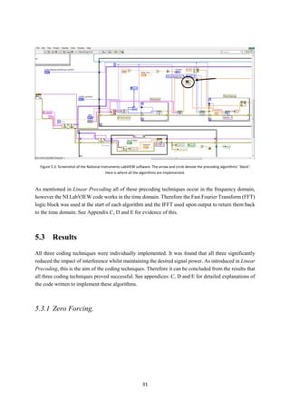
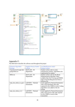
Figure 5.3 shows a screenshot of National Instrument’s ‘usrp_nxn_mimo_tx_que.vi’ transmitter side
code provided alongside the USRPs. The code runs everything required for real-world transmission. It
runs all antenna configurations, bit generation, modulation, OFDM, pulse shaping etc. The objective of
this part of the project was to add the coding techniques to this original code. The coding techniques
were written within the circled block diagram seen in Figure 5.3.
Figure 5.2: Screenshot of the ‘Front Panel’ in the LabVIEW USRP software

31
As mentioned in Linear Precoding all of these precoding techniques occur in the frequency domain,
however the NI LabVIEW code works in the time domain. Therefore the Fast Fourier Transform (FFT)
logic block was used at the start of each algorithm and the IFFT used upon output to return them back
to the time domain. See Appendix C, D and E for evidence of this.
5.3 Results
All three coding techniques were individually implemented. It was found that all three significantly
reduced the impact of interference whilst maintaining the desired signal power. As introduced in Linear
Precoding, this is the aim of the coding techniques. Therefore it can be concluded from the results that
all three coding techniques proved successful. See appendices: C, D and E for detailed explanations of
the code written to implement these algorithms.
5.3.1 Zero Forcing.
Figure 5.3: Screenshot of the National Instruments LabVIEW software. The arrow and circle denote the precoding algorithms’ ‘block’.
Here is where all the algorithms are implemented.

32
The Zero Forcing algorithm was the first to be implemented. As can be seen in Figure 5.4, the algorithm
is originally turned off (hence the interference occurring at an average of approximately 0.11dBm) this
interference signal is mainly Co-Channel Interference.
Once turned on, the interference signal was found to immediately drop very close to zero (see red arrows
in Figure 5.4). This can be seen in Figure 5.5 by the interference values in the Received Signals matrix
(h01 and h10) which have dropped very close to zero. The absolute values for these are combined to
create the interference signal whilst the absolute desired signal values (h00 and h11) are combined to
create the desired signal values. These values are then used to form the graphs. (Note the received
signals are complex values, hence the need to find the absolute values to ensure no power lost).
We can check to see if the Zero Forcing is working ideally by multiplying the precoding matrix (𝑊 =
𝐻−1
) by the channel matrix, 𝐻. In an ideal case, the identity matrix should be formed (see Coding
Algorithms) Figure 5.6 shows an example when the Zero Forcing algorithm is turned ON. The matrix
formed is very close to the identity matrix but not perfect. This is because the USRPs cannot update the
CSI information instantaneously.
Figure 5.4: Screenshot of the Zero Forcing Front Panel Showing Total Signal and Interference Signal graphs
over time. Zero Forcing is initially OFF, then turned ON, and then turned OFF again.
ON
ON
OFF
OFF
Figure 5.5: Screenshot of Received Signals Matrix when Zero Forcing is turned ON
Figure 5.6: A Screenshot of the ‘Check – Identity’ matrix when the Zero Forcing algorithm is turned ON.

33
As previously eluded, the Zero Forcing technique does not account for the AWGN in the channel.
However it can be seen that once Zero Forcing is turned on, the interference signal drops very close to
zero. This implies that there is very little AWGN in the channel. This can be expected due to the setup
of the experiment. The transmitters and receivers are so close to each other and have a line of sight (see
Figure 5.1). If the USRPs were to be moved further apart from each other the amount of AWGN should
increase. This would cause very different results.
5.3.2 Block Diagonalisation
Meanwhile, Figure 5.6 shows that the Block Diagonalisation algorithm also manages to heavily mitigate
the interference signal very close to zero once turned on. Block Diagonalisation achieves this whilst
maintaining a desired signal power level of approximately 2.8dBm. The received signals matrix
(circled) shows that the two interference values (h01 and h10) are pushed very close to zero when the
algorithm is turned ON. Hence it can be concluded that the algorithm works.
Figure 5.8 shows the received signals when the algorithm is OFF. From this it can be seen how well the
Block Diagonalisation technique has mitigated the interference values whilst maintaining the desired
signal values.
The precoding matrix at the time of the screenshot is also shown in Figure 5.7. This precoding matrix,
at the time of the screenshot, is multiplied by the symbols to be transmitted. Then once the signal is
received (and the CSI has interacted with it), the interference signals have been mitigated close to zero.
The code written to achieve these results can be seen in Appendix D.
Figure 5.7: Screenshot of the Block Diagonalisation coding technique. The interference is forced very close to zero once turned ON.
Figure 5.8: Screenshot of the Received Signals matrix when Block Diagonalisation is OFF.

34
5.3.3 Signal to Leakage Noise Ratio
Finally, the SLNR algorithm was implemented (see Appendix E). Unlike the other techniques, the aim
is mitigate the amount of desired signal leaked onto undesired receivers. Figure 5.9 shows that when
the SLNR algorithm is turned ON the interference signal power immediately falls from an average of
approximately 0.13dBm to approximately 0.02dBm whilst maintaining a desired signal average of
approximately 2.75dBm.
Figure 5.10 shows the received signals matrix before the SLNR algorithm is turned ON. The
interference
As SLNR is a probability based algorithm a prior probability is computed for the precoding matrix. As
the CSI is not instantaneous, the SLNR algorithm predicts the precoding matrix, 𝑊. This prediction is
not always completely accurate and hence, the interference signal power is not driven as close to zero
as the Zero Forcing or Block Diagonalisation algorithms. From this, we can conclude that the SLNR
algorithm works optimally when the CSI can be easily predicted so for example in a reliable
communication environment and will work poorly in an environment where CSI has large fluctuations,
so for example in a busy city or if the user is moving quickly (ie in a car).
5.4 Summary
Overall, it is difficult to compare and contrast the three coding techniques studied for this hardware
validation because the algorithms can’t be run simultaneously and as such all algorithms are working
with different CSI values. However, it was found that all three coding techniques mitigate all
interference very well.
Figure 5.9: Screenshot of the Block Diagonalisation coding technique. The interference is forced very close to zero once turned ON.
Figure 5.10: SLNR turned OFF
ON
OFF

35
From the results, we can tell that there is very little AWGN in the channel. This is because the Zero
Forcing and Block Diagonalisation algorithms push the interference so low and we know that neither
of these techniques are able to cancel this AWGN.

37
Chapter 6 - Conclusions
Today, the challenge proposed of the telecoms bottleneck is fast approaching. A huge capacity jump is
required and fast whilst maintaining Quality of Service. Addressing this challenge has revealed some
exciting conclusions. The objective was to analyse coding techniques used to mitigate the Co-Channel
Interference problem present in Multi-User MIMO systems through an initial software model and to
then use hardware to back up theoretical conclusions.
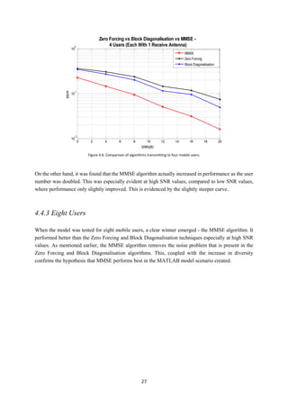
These were tested under different Multi-User scenarios with differing levels of success. Encouragingly,
it was found that all coding techniques employed brought significant reductions in interference.
Mitigation of interference can be successfully achieved and as such MIMO technology is a suitable
solution to the telecoms bottleneck challenge.
The MATLAB software simulation of these algorithms was tested upon increasing user numbers and
hence Multi-User scenarios. It was found that of the three algorithms tested, the Minimum Mean Square
Error (MMSE) algorithm achieves the best bit error rate performance, especially as user number
increases. This is because the MMSE algorithm accounts for the AWGN noise problem present in the
channel, unlike the other two algorithms studied (Zero Forcing and Block Diagonalisation) as discussed
in Comparison of Algorithms. When we also take into account the MMSE’s algorithms use of spatial
diversity (so that more desired signal streams are arriving at the receiver) greater Quality of Service and
Bit Error Rate performance can be achieved.
These theoretical conclusions were successfully verified using the USRP hardware provided by
National Instruments. However, it was found that the MMSE algorithm only performs well at a bit level.
In contrast, the SLNR algorithm employs a similar method but operates effectively at a packet level.
Therefore it was considered to be the more appropriate to use in the hardware validation.
Limitations with the hardware validation design made it difficult to compare the three coding techniques
used in the LabVIEW environment. However, it was revealed that all three mitigated almost all
interference in a simple 2x2 MISO real-world propagation environment. In Hardware Validation
analysis proved that in the specific case tested (2x2, high SNR, instantaneous CSI) the Zero Forcing
and Block Diagonalisation techniques work best. However, as MIMO size increases and SNR drops, it
has been ascertained that the SLNR algorithm will provide more effective results [30]. Again, this is
because the SLNR algorithm (like MMSE) is a probability based algorithm and tries to mitigate the
AWGN present unlike the Zero Forcing and Block Diagonalisation methods. In summary, the hardware
validation successfully endorsed all the theoretical conclusions proposed in Software Simulation.
The broad assumption made throughout the project was that each transmitter knows the Channel State
Information perfectly and instantaneously. In reality this is unlikely to be the case, as the coding
techniques work in the frequency domain, hence use FDD to feedback the CSI (see Channel State
Information & Feedback). Ultimately the project has proved that fundamentally with perfect CSI, these
coding techniques work well. As discussed in Further Work, it has been demonstrated that both the
Minimum Mean Square Error and the Block Diagonalisation algorithms outperform Zero Forcing with
imperfect Channel State Information and as such back up the conclusions made from this project.

38
To summarise, the selection of algorithm depends entirely on the scenario. If low computational
complexity is required with little to zero AWGN present in the channel, Zero Forcing is the optimum
solution. If multiple receive antennas are present for each separate Mobile User, Block Diagonalisation
is the preferred method. If performance is paramount (ie no errors, reliable connection, high QoS) the
MMSE or SLNR solution is more effective to achieve the highest spectral efficiency possible; the
MMSE in preference to SLNR if at a bit level and vice versa if at a packet level.

39
Chapter 7 - Further Work
7.1 Overview
This chapter introduces further work that could be carried out to expand on this project in the future.
Some exciting areas currently receiving a lot of attention are also considered.
7.2 Multiple Receive Antenna’s per User
Each user has more than one receive antenna. As smart antenna technology is progressing it is becoming
more and more common for the Mobile User device to have more than one receive antenna. All of this
has been previously limited to one transmit and one receive antenna systems due to the additional levels
of processing power needed. It has been found that the when the user has more than one receive antenna,
the Block Diagonalisation algorithm performs best [31]. Further work could test this hypothesis using
the MATLAB model created. The proposition of multiple receive antennas could also be tested in the
hardware, however different USRPs would be needed due to limitations of the USRP-2920.
7.3 Test with Better USRPs
For the hardware validation side of the project we have only tested the algorithms in a two transmitter,
two receiver environment. Further work could connect multiple USRPs together to create larger
dimension propagation environments. The National Instruments LabVIEW testbed can accommodate
up to eight USRPs (hence an 8x8 propagation environment). From this, the theoretical results created
in the MATLAB model could be compared to the real world model. This would validate the MATLAB
model whilst also providing valuable conclusions to the LabVIEW hardware model.
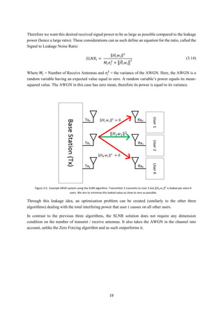
Even better further work could be used to implement these coding algorithms upon more advanced
USRPs. The USRP RIO’s could be used for example [32]. The advantages of using the more advanced
Figure 7.1: The NI USRP Rio’s in action in the Bristol University CSN Laboratory. Here, up to 128 transmit and receive antennas can be tested.

40
USRPs are that we can achieve much larger dimension MIMO configurations (up to 128 transmit and
receive antennas in the Bristol University lab). FPGA algorithms can also be implemented. These
scenarios are closer aligned to future fifth generation wireless communication systems and as such
provide a more rigorous and accurate test of the coding techniques.
7.4 Introduce More Channel Scenarios
As discussed in Conclusions, throughout the whole project a big assumption made is that the transmitter
has perfect, instantaneous Channel State Information. In multiuser scenarios, this is thought to be crucial
for the multiplexing gains offered by interference alignment and the subsequent coding techniques. It
is known that the performance of these techniques are very sensitive to inaccuracies in the CSI [33]. In
reality, perfect instantaneous Channel State Information is very hard to obtain. This is especially true
in Frequency Division Duplex systems used throughout this project (see Channel State Information &
Feedback) where the CSI is obtained via feedback from the receiver. Obviously, the time for the receiver
to relay this channel state matrix back to the transmitter is not instantaneous. If this feedback delay is
very large compared to the channel coherence time, the Channel State Information received will not be
accurate or reliable. This feedback process leads to two types of error: Quantisation Error and Delay
[34].
Further work to this project could study this ‘Outdated CSI’ and how to use it to predict the current state
of the CSI. One method proposed in [34] proposes the communication scheme to be performed in two
phases, taking three time slots for the 2x2 MISO configuration studied in Figure 7.2.
The method studied in [34] for a 2x2 MISO example achieves a Degree of Freedom of 2/3. This is a
remarkable improvement on previous TDMA techniques that can only manage a Degree of Freedom
of 1/3 in an equivalent scenario.
Further work on this could fall two ways. Academically, the Outdated CSI theory could be analysed
and perhaps improved upon. Or, practically, it could be to implement the method proposed in Figure
7.2 into the LabVIEW and USRP model. From this, the LabVIEW model will be even more like a real
world propagation environment.
Figure 7.2: An achievable scheme for computing CSI when it is outdated. The above diagram is a 2x2 MISO case. (From M. Maddah-Ali and
D. Tse, 2010) [34]

41
Bibliography
[1] Mark Cudak – Nokia Networks’ principal research specialist. Taken from an article by Tereza Pultarova in
E&T: “5G Excitement at Mobile World Congress”
[2] Simon Saunders, Director of Technology at Real Wireless, and independent consultancy based in Pulborough,
UK. From a BBC article by Frank Swain: “Will we ever… face a wireless ‘spectrum crunch’?” Available at:
http://www.bbc.com/future/story/20131014-are-we-headed-for-wireless-chaos
[3] Professor. Andrew Nix, University of Bristol, 'Mobile Communications Notes', Electronic & Electrical
Engineering Department, Bristol, 2015.
[4] Wong & Lok: “Theory of Digital Communications”. Ch 4 – ISI & Equalization. pp. 4.2
[5] V. Cadambe, S. Jafar and S. Shamai, 'Interference Alignment on the Deterministic Channel and Application
to Fully Connected Gaussian Interference Networks', IEEE Transactions on Information Theory, vol. 55, no. 1,
pp. 269-274, 2009.
[6] H. Q. Ngo ‘Performance Bounds for Very Large Multiuser MIMO systems’, Linköping: Linköping University
Electronic Press, 2012
[7] Godavarti, M. (n.d.). Diversity and Degrees of Freedom in Wireless Communications. Available at:
http://web.eecs.umich.edu/~hero/Preprints/icassp2002_godv.pdf
[8] Bandemer, B., Haardt, M. and Visuri, S. (2006). Linear MMSE Multi-User MIMO Downlink Precoding for
Users with Multiple Antennas. 2006 IEEE 17th International Symposium on Personal, Indoor and Mobile Radio
Communications.
[9] LTE Quality of Experience. (2013). JDSU, p.7.
[10] Radio-electronics.com, (2015). What is QAM. [online] Available at: http://www.radio-
electronics.com/info/rf-technology-design/quadrature-amplitude-modulation-qam/what-is-qam-tutorial.php
[Accessed 23 Apr. 2015].
[11]S. Sesia, M. Baker and I. Toufik, LTE, the UMTS long term evolution. Chichester, U.K.: Wiley, 2009.
[12] Hagerman, B. (1995). Downlink relative co-channel interference powers in cellular radio systems. 1995 IEEE
45th Vehicular Technology Conference. Countdown to the Wireless Twenty-First Century.
[13] A Medra, T Davidson “Widely Linear Interference Alignment Precoding” IEEE Transactions on Information
Theory. McMaster University, Canada. pp.464-468. June 2014
[14] M. Maddah-Ali, A. Motahari and A. Khandani, 'Communication Over MIMO X Channels: Interference
Alignment, Decomposition, and Performance Analysis', IEEE Transactions on Information Theory, vol. 54, no.
8, pp. 3457-3470, 2008.
[15] V. Cadambe, S. Jafar, ‘Interference alignment and degrees of freedom of the K-user interference channel,’
IEEE Trans. Inf. Theory. Vol 54, pp. 3425-3441, Aug 2008.
[16] F. Kaltenberger, M. Kountouris, L. Cardoso, R. Knopp and D. Gesbert, 'Capacity of linear multi-user MIMO
precoding schemes with measured channel data', 2008 IEEE 9th Workshop on Signal Processing Advances in
Wireless Communications, 2008.

42
[17] Uk.mathworks.com, (2015). Moore-Penrose pseudoinverse of matrix. [online] Available at:
http://uk.mathworks.com/help/matlab/ref/pinv.html [Accessed 23 Apr. 2015].
[18] T. Gou and S. Jafar, 'Degrees of Freedom of the K User M x N MIMO Interference Channel', IEEE
Transactions on Information Theory, vol. 56, no. 12, pp. 6040-6057, 2010.
[19] D. Ben Cheikh, J. Kelif, M. Coupechoux and P. Godlewski, 'Multicellular Zero Forcing Precoding
Performance in Rayleigh and Shadow Fading', 2011 IEEE 73rd Vehicular Technology Conference (VTC Spring),
2011.
Communications.
[21] Mathworld.wolfram.com, (2015). Eigen Decomposition Theorem -- from Wolfram MathWorld. [online]
Available at: http://mathworld.wolfram.com/EigenDecompositionTheorem.html [Accessed 23 Apr. 2015].
[22] N. Chiurtu, B. Rimoldi and E. Telatar, 'On the capacity of multi-antenna Gaussian channels', Proceedings.
2001 IEEE International Symposium on Information Theory (IEEE Cat. No.01CH37252), 2001.
Communications.
[24] M. Sadek, A. Tarighat and A. Sayed, 'A Leakage-Based Precoding Scheme for Downlink Multi-User MIMO
Channels', IEEE Transactions on Wireless Communications, vol. 6, no. 5, pp. 1711-1721, 2007.
[25] LTE Quality of Experience. (2013). JDSU, p.13.
[26] Ni.com, 'USRP - National Instruments', 2015. [Online]. Available: http://www.ni.com/sdr/usrp/. [Accessed:
21- Apr- 2015].
[27] Sine.ni.com, 'NI USRP-2920 - National Instruments', 2015. [Online]. Available:
http://sine.ni.com/nips/cds/view/p/lang/en/nid/212995. [Accessed: 21- Apr- 2015].
[28] Ni.com, (2015). NI LabVIEW. [online] Available at: http://www.ni.com/labview/ [Accessed 23 Apr. 2015].
[29] 4G, '4G frequencies in the UK: What you need to know', 2015. [Online]. Available: http://www.4g.co.uk/4g-
frequencies-uk-need-know/. [Accessed: 21- Apr- 2015].
[30] M. Sadek, A. Tarighat and A. Sayed, 'A Leakage-Based Precoding Scheme for Downlink Multi-User MIMO
Channels', IEEE Transactions on Wireless Communications, vol. 6, no. 5, pp. 1711-1721, 2007.
[31] R. Chen, Z. Shen, J. Andrews and R. Heath, 'Multimode Transmission for Multiuser MIMO Systems With
Block Diagonalization', IEEE Trans. Signal Process., vol. 56, no. 7, pp. 3294-3302, 2008.
[32]Sine.ni.com, (2015). NI USRP RIO - National Instruments. [online] Available at:
http://sine.ni.com/nips/cds/view/p/lang/en/nid/212991 [Accessed 23 Apr. 2015].
[33] M. Maddah-Ali, A. Motahari and A. Khandani, 'Communication Over MIMO X Channels: Interference
Alignment, Decomposition, and Performance Analysis', IEEE Transactions on Information Theory, vol. 54, no.
8, pp. 3457-3470, 2008.
[34] M. Maddah-Ali and D. Tse, 'Completely stale transmitter channel state information is still very useful', 2010
48th Annual Allerton Conference on Communication, Control, and Computing (Allerton), 2010.

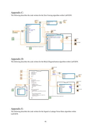
43
Appendix
Appendix A:
The following describes the MATLAB code used for the Software Simulation mentioned throughout
this project.
clear all
Nt=4; Nr=4;
SNR=[0:2:20];
channel_n=100*ones(1,length(SNR));
error_mmselinp=zeros(1,length(SNR));
error_zflinp=zeros(1,length(SNR));
error_bdlinp=zeros(1,length(SNR));
for loop_ebno=1:length(SNR)
snr=10.^(SNR(loop_ebno)/10); % SNR in decimel
ea=1; % Power of one transmitter
es=ea*Nt; % Power of all transmitters
sigma_n2=es/snr; % Power / SNR
num=10;
for loop_channel=1:channel_n(loop_ebno)
% *** Create Channel ***
H=sqrt(1/2)*(randn(Nr,Nt)); %+j*randn(Nr,Nt))
% *** Create Precoding Matrix ***
mmse_F=H'*inv(H*H'+sigma_n2/ea*eye(Nt));
zf_F=H'*inv(H*H');
F = BDFct(Nt,Nr,H);
bd_F = cell2mat(F);
% *** Create Normalisation ***
beta_mmse=sqrt(es/norm(mmse_F,'fro').^2);
beta_zf=sqrt(es/norm(zf_F,'fro').^2);
beta_bd=sqrt(es/norm(bd_F,'fro').^2);
% *** Precode = F*normalisation ***
F_mmse=beta_mmse*mmse_F;
F_zf=beta_zf*zf_F;
F_bd=beta_bd*bd_F;
for loop_num=1:num
% *** Generate symbols - QPSK ***
gen_u=sign(randn(Nt,1))+j*sign(randn(Nt,1));
u=sqrt(1/2)*gen_u;
% *** Precode x Symbols ***
x_mmse=F_mmse*u;
x_zf=F_zf*u;
x_bd=F_bd*u;
% *** Received Signals (with AWGN) ***
y_mmse = H*awgn(x_mmse,SNR(loop_ebno));
y_zf = H*awgn(x_zf,SNR(loop_ebno));
y_bd = H*awgn(x_bd,SNR(loop_ebno));
% BD need decoding process
Deco_bd=inv(H*F_bd);
% *** Normalise again ***
r_mmse=1/beta_mmse*y_mmse;
r_zf=1/beta_zf*y_zf;
r_bd=1/beta_bd*Deco_bd*y_bd;
% *** Round received symbols (Hard Decision Decoder) ***
rev_data_mmse=sign(real(r_mmse))+j*sign(imag(r_mmse)); % QPSK
rev_data_zf=sign(real(r_zf))+j*sign(imag(r_zf));
rev_data_bd=sign(real(r_bd))+j*sign(imag(r_bd));

44
% *** Find Errors - compares gen_u and rev_data returns number of errors***
error_mmselinp(1,loop_ebno)=error_mmselinp(1,loop_ebno)+sum(((abs(rev_data_mmse-
gen_u)).^2)/4);
error_zflinp(1,loop_ebno)=error_zflinp(1,loop_ebno)+sum(((abs(rev_data_zf-
gen_u)).^2)/4);
error_bdlinp(1,loop_ebno)=error_bdlinp(1,loop_ebno)+sum(((abs(rev_data_bd-
gen_u)).^2)/4);
end
end
% *** Create BER **
ber_mmselinp(1,loop_ebno)=error_mmselinp(1,loop_ebno)/(num*Nt*2*channel_n(loop_ebno));
ber_zflinp(1,loop_ebno)=error_zflinp(1,loop_ebno)/(num*Nt*2*channel_n(loop_ebno));
ber_bdlinp(1,loop_ebno)=error_bdlinp(1,loop_ebno)/(num*Nt*2*channel_n(loop_ebno));
end
% *** Plot Graphs ***
semilogy(SNR,ber_mmselinp,'o-r');
hold on
semilogy(SNR,ber_zflinp,'*-k');
hold on
semilogy(SNR,ber_bdlinp,'*-b');
grid on;
xlabel('SNR(dB)');ylabel('BER');
title('Zero Forcing vs MMSE vs BD (QPSK)')
leg1='MMSE';
leg2='ZF';
leg3='BD';
legend(leg1,leg2,leg3);
Appendix B:
The following describes a separate function created to simulate the Block Diagonalisation function
and works in accordance with Appendix A once called.
% *** BD Function ***
function [F] = BDFct(Nt,Nr,H)
for h=1:Nt
H_BD{1,h}=H(h,:);
end
Ht=H_BD';
for aim_user=1:Nr
userant_num = 1;
interf_channel = [];
interf_user = setdiff(1:Nr,aim_user); % Returns values in 1:user_num that are not in
aim_user
% *** Create Interfering Channel Matrix ***
for interf_num=1:Nr-1
interf_channel=[interf_channel;H_BD{interf_user(interf_num)}];
end;
% *** SVD Operation x2 to create F ***
[U, D, V]=svd(interf_channel);
V_j0=V(:,(interf_num*userant_num+1):end); % Find V_k1 (the first left eigenvectors)
Hs=H_BD{aim_user}*V_j0;
[U1, D1, V1]=svd(Hs); % Implement SVD operation on Hj (H{aim_user}) and V_j0
V1_j1=V1(:,1:userant_num); % Find V1_j1 (the first left eigenvectors)
F{aim_user}=V_j0*V1_j1;
end

45
Appendix C:
The following describes the code written for the Zero Forcing algorithm within LabVIEW.
Appendix D:
The following describes the code written for the Block Diagonalisation algorithm within LabVIEW.
Appendix E:
The following describes the code written for the Signal to Leakage Noise Ratio algorithm within
LabVIEW.

46
Appendix F:
The table below describes the software used throughout the project.
Filename/Algorithm/
Package
Supplier/Source/Author/
website
Use/Modifications made/
Student written
TransmissionUsingCodin
gAlgorithms.m
MATLAB – EE
Department
Student written code to create
transmission scenario. Algorithms also
implemented by student/
BDFct.m MATLAB – EE
Department
Student written code for the Block
Diagonalisation algorithm. More
complex than Zero Forcing and MMSE
(due to the decoding process) hence a
different file.
usrp_nxn_mimo_tx_que.v
i
LabVIEW – National
Instruments
Code supplied by National Instruments.
This is the transmitter side code
required for the USRPs to work. Coding
algorithms were added to this for
testing.
usrp_nxn_mimo_rx.vi LabVIEW – National
Instruments
Code supplied by National Instruments.
This is the receiver side code required
for the USRPs to receive data
transmitted.

47
zero_forcing.vi LabVIEW – National
Instruments
Student written code for the Zero
Forcing algorithm
block_diagonalisation.vi LabVIEW – National
Instruments
Student written code for the Block
Diagonalisation algorithm
slnr.vi LabVIEW – National
Instruments
Student written code for the Signal to
Leakage Noise Ratio algorithm
Appendix G:
The CD attached to this report includes all finished working code used throughout the project. It also
includes: Interim Report, Poster and videos of the working algorithms in action.

MartinDickThesis

Recommended

Recommended

More Related Content

What's hot

What's hot (20)

Viewers also liked

Viewers also liked (6)

Similar to MartinDickThesis

Similar to MartinDickThesis (20)

MartinDickThesis