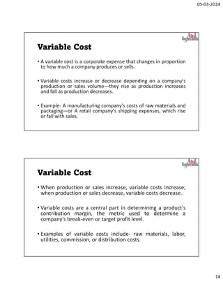
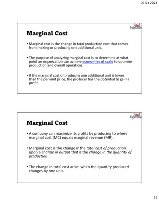
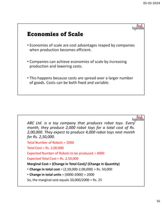
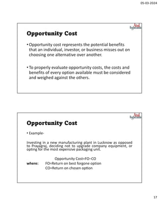
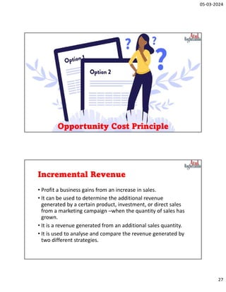
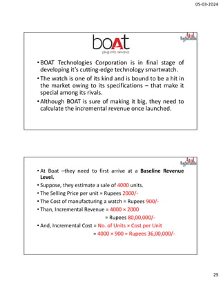
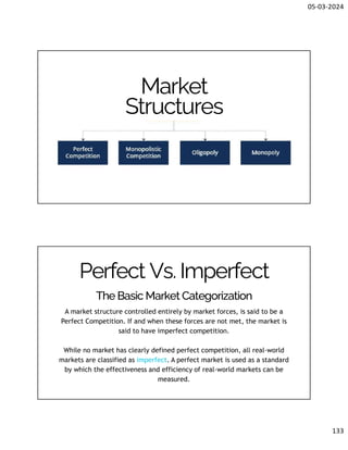
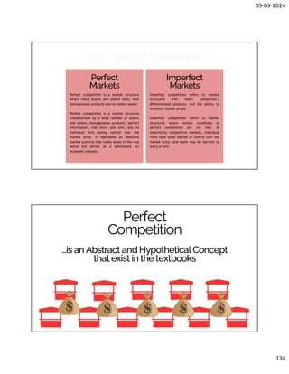
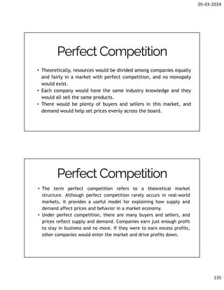
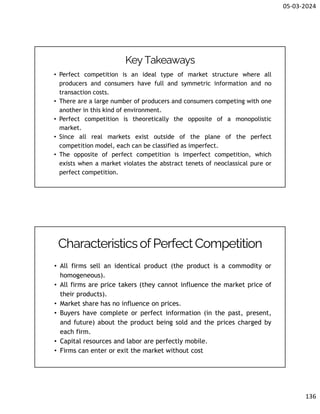
Download to read offline


![05-03-2024
79
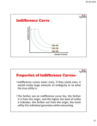
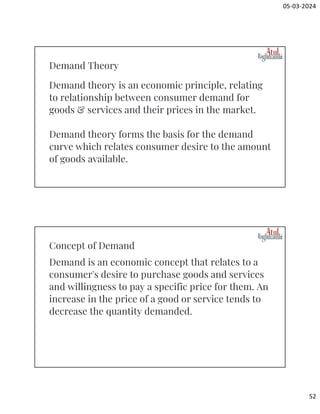
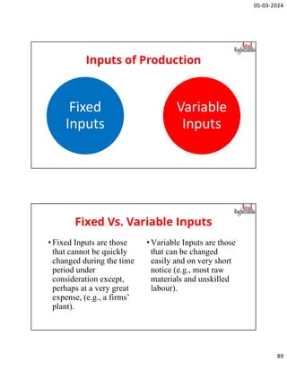
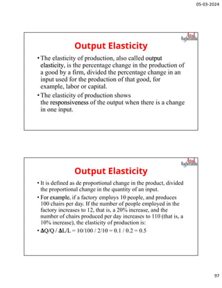
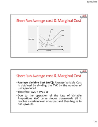
Supply Elasticity
•Es= [(Δq/q)×100] ÷ [(Δp/p)×100] = (Δq/q) ÷ (Δp/p)
•Δq= The change in quantity supplied
•q= The quantity supplied
•Δp= The change in price
•p= The price
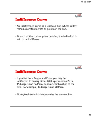
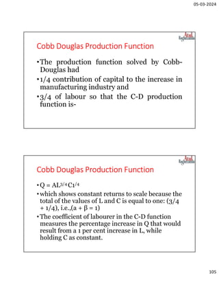
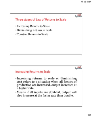
Types of Elasticity of Supply
•Perfectly Elastic Supply: A commodity becomes
perfectly elastic when its elasticity of supply is infinite.
This means that even for a slight increase in price, the
supply becomes infinite. For a perfectly elastic supply,
the percentage change in the price is zero for any
change in the quantity supplied.
•More than Unit Elastic Supply: When the percentage
change in the supply is greater than the percentage
change in price, then the commodity has the price
elasticity of supply greater than 1.](https://image.slidesharecdn.com/managerialeconomicscombinedcompressed-240322034821-bdea5f2c/85/Managerial-Economics-Combined_compressed-pdf-79-320.jpg)


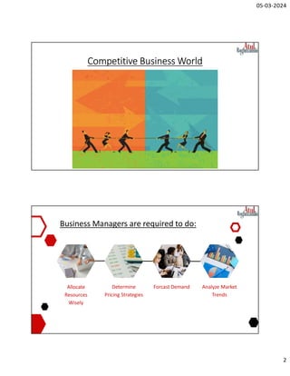
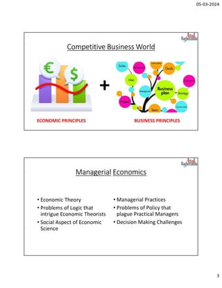
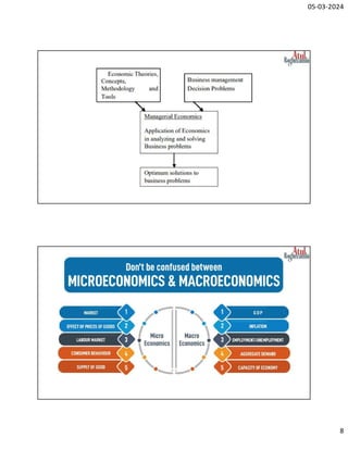
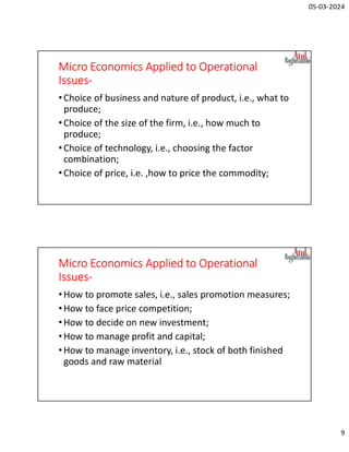
This document provides an overview of managerial economics and key economic concepts for managers. It discusses: 1) The global trend of increasing new businesses starting each year from 2012 to 2022. 2) Key tasks for business managers like allocating resources, determining pricing strategies, and analyzing market trends. 3) Definitions of managerial economics focusing on applying economic theory to managerial decision-making and bridging economic and business practices. 4) Fundamental economic concepts like scarcity of resources, opportunity cost, sunk cost, marginal cost, economies of scale, fixed and variable costs that managers must consider in decision-making.


