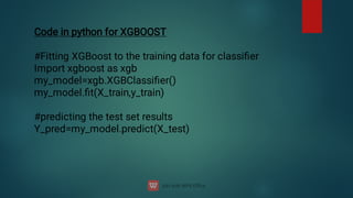
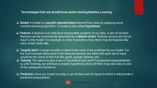
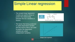
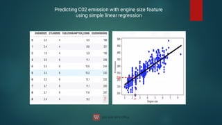
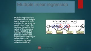
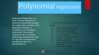
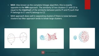
The document discusses the concept of machine learning, which allows computers to learn from data without explicit programming, contrasting it with traditional programming. It covers key terminologies, types of learning (supervised, unsupervised, and semi-supervised), and specific algorithms used in supervised learning like linear regression and decision trees. The document also highlights the importance of regression analysis and provides examples of its application in predicting outcomes.


![from sklearn import linear_model
regr = linear_model.LinearRegression()
train_x = np.asanyarray(train[['ENGINESIZE']])
train_y = np.asanyarray(train[['CO2EMISSIONS']])
regr.fit (train_x, train_y)
# The coefficients
print ('Coefficients: ', regr.coef_)
print ('Intercept: ',regr.intercept_)](https://image.slidesharecdn.com/machinelearning-240622113900-3ccd8cd9/85/Machine-Learning-deep-learning-artificial-15-320.jpg)

![from sklearn import linear_model
regr = linear_model.LinearRegression()
train_x = np.asanyarray(train[['ENGINESIZE','CYLINDERS']])
train_y = np.asanyarray(train[['CO2EMISSIONS']])
regr.fit (train_x, train_y)
# The coefficients
print ('Coefficients: ', regr.coef_)
print ('Intercept: ',regr.intercept_)](https://image.slidesharecdn.com/machinelearning-240622113900-3ccd8cd9/85/Machine-Learning-deep-learning-artificial-18-320.jpg)
![from sklearn.preprocessing import PolynomialFeatures
from sklearn import linear_model
train_x = np.asanyarray(train[['ENGINESIZE','CYLINDERS']])
train_y = np.asanyarray(train[['CO2EMISSIONS']])
test_x = np.asanyarray(test[['ENGINESIZE']])
test_y = np.asanyarray(test[['CO2EMISSIONS']])
poly = PolynomialFeatures(degree=2)
train_x_poly = poly.fit_transform(train_x)
train_x_poly.shape](https://image.slidesharecdn.com/machinelearning-240622113900-3ccd8cd9/85/Machine-Learning-deep-learning-artificial-21-320.jpg)


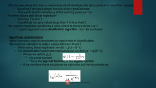
![•
•
•
How does the sigmoid function look like
Crosses 0.5 at the origin, then flattens out]
Asymptotes at 0 and 1](https://image.slidesharecdn.com/machinelearning-240622113900-3ccd8cd9/85/Machine-Learning-deep-learning-artificial-33-320.jpg)


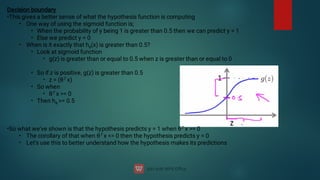
![Consider,
hθ
(x) = g(θ0
+ θ1
x1
+ θ2
x2
)
•
•
•
•
•
•
•
•
•
•
•
•
•
•
•
So, for example
θ0
= -3
θ1
= 1
θ2
= 1
So our parameter vector is a column vector with the above values
So, θT is a row vector = [-3,1,1]
What does this mean?
The z here becomes θT x
We predict y = 1 if
-3x0
+ 1x1
+ 1x2
= 0
-3 + x1
+ x2
= 0
We can also re-write this as
If (x1
+ x2
= 3) then we predict y = 1
If we plot
x1
+ x2
= 3 we graphically plot our decision boundary](https://image.slidesharecdn.com/machinelearning-240622113900-3ccd8cd9/85/Machine-Learning-deep-learning-artificial-37-320.jpg)
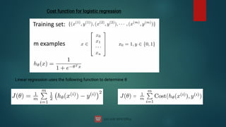
![hθ(x) = g(θ0 + θ1x1+ θ3x1
2 + θ4x2
2)
•
•
•
•
•
Say θT was [-1,0,0,1,1] then we say;
Predict that y = 1 if
-1 + x1
2 + x2
2 = 0
or
x1
2 + x2
2 = 1
If we plot x1
2 + x2
2 = 1](https://image.slidesharecdn.com/machinelearning-240622113900-3ccd8cd9/85/Machine-Learning-deep-learning-artificial-38-320.jpg)


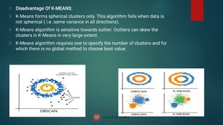


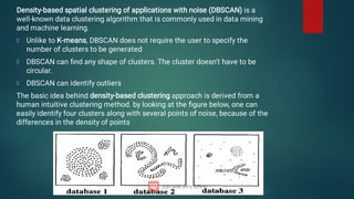
![DBSCAN algorithm has two parameters:
ɛ: The radius of our neighborhoods around a data point p.
minPts: The minimum number of data points we want in a neighborhood to define a cluster.
Using these two parameters, DBSCAN categories the data points into three categories:
Core Points: A data point p is a core point if Nbhd(p,ɛ) [ɛ-neighborhood of p] contains at least
minPts ; |Nbhd(p,ɛ)| = minPts.
Border Points: A data point *q is a border point if Nbhd(q, ɛ) contains less than minPts data
points, but q is reachable from some core point p.
Outlier: A data point o is an outlier if it is neither a core point nor a border point. Essentially,
this is the “other” class.](https://image.slidesharecdn.com/machinelearning-240622113900-3ccd8cd9/85/Machine-Learning-deep-learning-artificial-103-320.jpg)


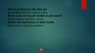
![Code in python for getting optimal hyperparameter using
gridsearch for support vector machine:
#importing svm from svc library
from sklearn.svm import SVC
Classifier=SVC()
#To import gridsearcv class from sklearn library
from sklearn.model_selection import GridSearchCV
#creating a list of dictonarties that need to be inputed for grid search
parameters=[{'C':[1,10,100,1000],'kernel':['linear']},{'C':[1,10,100,1000],'kernel':['rbf'
],'gamma':[0.5,0.1,0.01,0.001]}]
#creating grid search object
gridsearch=GridSearchCV(estimator=classifier,param_grid=parameters,
scoring='accuracy',cv=10,n_jobs=-1)
#fitting gridsearch with data set
gd=gridsearch.fit(X_train,y_train)](https://image.slidesharecdn.com/machinelearning-240622113900-3ccd8cd9/85/Machine-Learning-deep-learning-artificial-111-320.jpg)