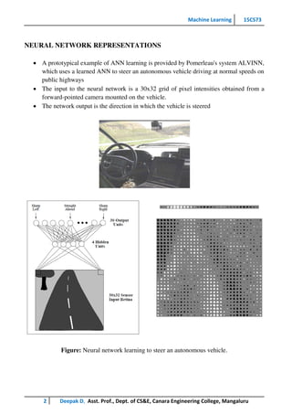
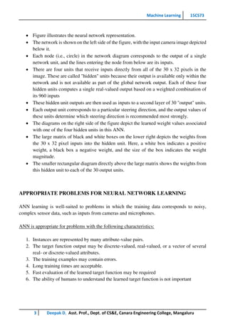
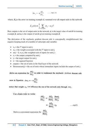
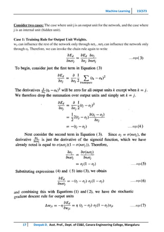
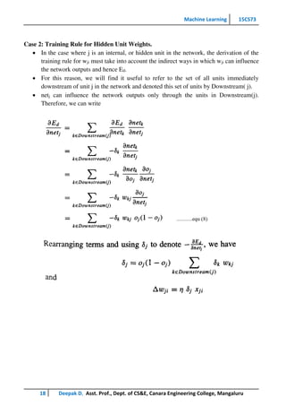
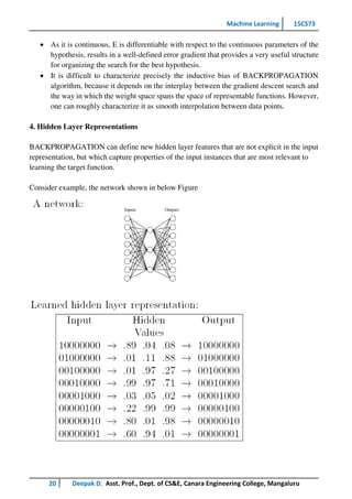
SlideShare a Scribd company logo
Machine Learning 15CS73
1 Deepak D, Asst. Prof., Dept. of CS&E, Canara Engineering College, Mangaluru
MODULE 3
ARTIFICIAL NEURAL NETWORKS
INTRODUCTION
Artificial neural networks (ANNs) provide a general, practical method for learning real-valued,
discrete-valued, and vector-valued target functions.
Biological Motivation
 The study of artificial neural networks (ANNs) has been inspired by the observation that
biological learning systems are built of very complex webs of interconnected Neurons
 Human information processing system consists of brain neuron: basic building block
cell that communicates information to and from various parts of body
Facts of Human Neurobiology
 Number of neurons ~ 1011
 Connection per neuron ~ 10 4 – 5
 Neuron switching time ~ 0.001 second or 10 -3
 Scene recognition time ~ 0.1 second
 100 inference steps doesn’t seem like enough
 Highly parallel computation based on distributed representation
Properties of Neural Networks
 Many neuron-like threshold switching units
 Many weighted interconnections among units
 Highly parallel, distributed process
 Emphasis on tuning weights automatically
 Input is a high-dimensional discrete or real-valued (e.g, sensor input )
Machine Learning 15CS73
2 Deepak D, Asst. Prof., Dept. of CS&E, Canara Engineering College, Mangaluru
NEURAL NETWORK REPRESENTATIONS
 A prototypical example of ANN learning is provided by Pomerleau's system ALVINN,
which uses a learned ANN to steer an autonomous vehicle driving at normal speeds on
public highways
 The input to the neural network is a 30x32 grid of pixel intensities obtained from a
forward-pointed camera mounted on the vehicle.
 The network output is the direction in which the vehicle is steered
Figure: Neural network learning to steer an autonomous vehicle.
Machine Learning 15CS73
3 Deepak D, Asst. Prof., Dept. of CS&E, Canara Engineering College, Mangaluru
 Figure illustrates the neural network representation.
 The network is shown on the left side of the figure, with the input camera image depicted
below it.
 Each node (i.e., circle) in the network diagram corresponds to the output of a single
network unit, and the lines entering the node from below are its inputs.
 There are four units that receive inputs directly from all of the 30 x 32 pixels in the
image. These are called "hidden" units because their output is available only within the
network and is not available as part of the global network output. Each of these four
hidden units computes a single real-valued output based on a weighted combination of
its 960 inputs
 These hidden unit outputs are then used as inputs to a second layer of 30 "output" units.
 Each output unit corresponds to a particular steering direction, and the output values of
these units determine which steering direction is recommended most strongly.
 The diagrams on the right side of the figure depict the learned weight values associated
with one of the four hidden units in this ANN.
 The large matrix of black and white boxes on the lower right depicts the weights from
the 30 x 32 pixel inputs into the hidden unit. Here, a white box indicates a positive
weight, a black box a negative weight, and the size of the box indicates the weight
magnitude.
 The smaller rectangular diagram directly above the large matrix shows the weights from
this hidden unit to each of the 30 output units.
APPROPRIATE PROBLEMS FOR NEURAL NETWORK LEARNING
ANN learning is well-suited to problems in which the training data corresponds to noisy,
complex sensor data, such as inputs from cameras and microphones.
ANN is appropriate for problems with the following characteristics:
1. Instances are represented by many attribute-value pairs.
2. The target function output may be discrete-valued, real-valued, or a vector of several
real- or discrete-valued attributes.
3. The training examples may contain errors.
4. Long training times are acceptable.
5. Fast evaluation of the learned target function may be required
6. The ability of humans to understand the learned target function is not important
Machine Learning 15CS73
4 Deepak D, Asst. Prof., Dept. of CS&E, Canara Engineering College, Mangaluru
PERCEPTRON
 One type of ANN system is based on a unit called a perceptron. Perceptron is a single
layer neural network.
Figure: A perceptron
 A perceptron takes a vector of real-valued inputs, calculates a linear combination of
these inputs, then outputs a 1 if the result is greater than some threshold and -1 otherwise.
 Given inputs x through x, the output O(x1, . . . , xn) computed by the perceptron is
 Where, each wi is a real-valued constant, or weight, that determines the contribution of
input xi to the perceptron output.
 -w0 is a threshold that the weighted combination of inputs w1x1 + . . . + wnxn must surpass
in order for the perceptron to output a 1.
Sometimes, the perceptron function is written as,
Learning a perceptron involves choosing values for the weights w0 , . . . , wn . Therefore, the
space H of candidate hypotheses considered in perceptron learning is the set of all possible
real-valued weight vectors
Machine Learning 15CS73
5 Deepak D, Asst. Prof., Dept. of CS&E, Canara Engineering College, Mangaluru
Representational Power of Perceptrons
 The perceptron can be viewed as representing a hyperplane decision surface in the n-
dimensional space of instances (i.e., points)
 The perceptron outputs a 1 for instances lying on one side of the hyperplane and outputs
a -1 for instances lying on the other side, as illustrated in below figure
Perceptrons can represent all of the primitive Boolean functions AND, OR, NAND (~ AND),
and NOR (~OR)
Some Boolean functions cannot be represented by a single perceptron, such as the XOR
function whose value is 1 if and only if x1 ≠ x2
Example: Representation of AND functions
If A=0 & B=0 → 0*0.6 + 0*0.6 = 0.
This is not greater than the threshold of 1, so the output = 0.
If A=0 & B=1 → 0*0.6 + 1*0.6 = 0.6.
This is not greater than the threshold, so the output = 0.
If A=1 & B=0 → 1*0.6 + 0*0.6 = 0.6.
This is not greater than the threshold, so the output = 0.
If A=1 & B=1 → 1*0.6 + 1*0.6 = 1.2.
This exceeds the threshold, so the output = 1.
Machine Learning 15CS73
6 Deepak D, Asst. Prof., Dept. of CS&E, Canara Engineering College, Mangaluru
Drawback of perceptron
 The perceptron rule finds a successful weight vector when the training examples are
linearly separable, it can fail to converge if the examples are not linearly separable
The Perceptron Training Rule
The learning problem is to determine a weight vector that causes the perceptron to produce the
correct + 1 or - 1 output for each of the given training examples.
To learn an acceptable weight vector
 Begin with random weights, then iteratively apply the perceptron to each training
example, modifying the perceptron weights whenever it misclassifies an example.
 This process is repeated, iterating through the training examples as many times as
needed until the perceptron classifies all training examples correctly.
 Weights are modified at each step according to the perceptron training rule, which
revises the weight wi associated with input xi according to the rule.
 The role of the learning rate is to moderate the degree to which weights are changed at
each step. It is usually set to some small value (e.g., 0.1) and is sometimes made to decay
as the number of weight-tuning iterations increases
Drawback:
The perceptron rule finds a successful weight vector when the training examples are linearly
separable, it can fail to converge if the examples are not linearly separable.
Machine Learning 15CS73
7 Deepak D, Asst. Prof., Dept. of CS&E, Canara Engineering College, Mangaluru
Gradient Descent and the Delta Rule
 If the training examples are not linearly separable, the delta rule converges toward a
best-fit approximation to the target concept.
 The key idea behind the delta rule is to use gradient descent to search the hypothesis
space of possible weight vectors to find the weights that best fit the training examples.
To understand the delta training rule, consider the task of training an unthresholded perceptron.
That is, a linear unit for which the output O is given by
To derive a weight learning rule for linear units, specify a measure for the training error of a
hypothesis (weight vector), relative to the training examples.
Where,
 D is the set of training examples,
 td is the target output for training example d,
 od is the output of the linear unit for training example d
 E ( w
⃗⃗⃗⃗ ) is simply half the squared difference between the target output td and the linear
unit output od, summed over all training examples.
Visualizing the Hypothesis Space
 To understand the gradient descent algorithm, it is helpful to visualize the entire
hypothesis space of possible weight vectors and their associated E values as shown in
below figure.
 Here the axes w0 and wl represent possible values for the two weights of a simple linear
unit. The w0, wl plane therefore represents the entire hypothesis space.
 The vertical axis indicates the error E relative to some fixed set of training examples.
 The arrow shows the negated gradient at one particular point, indicating the direction in
the w0, wl plane producing steepest descent along the error surface.
 The error surface shown in the figure thus summarizes the desirability of every weight
vector in the hypothesis space
Machine Learning 15CS73
8 Deepak D, Asst. Prof., Dept. of CS&E, Canara Engineering College, Mangaluru
 Given the way in which we chose to define E, for linear units this error surface must
always be parabolic with a single global minimum.
Gradient descent search determines a weight vector that minimizes E by starting with an
arbitrary initial weight vector, then repeatedly modifying it in small steps.
At each step, the weight vector is altered in the direction that produces the steepest descent
along the error surface depicted in above figure. This process continues until the global
minimum error is reached.
Derivation of the Gradient Descent Rule
How to calculate the direction of steepest descent along the error surface?
The direction of steepest can be found by computing the derivative of E with respect to each
component of the vector w
⃗⃗⃗⃗ . This vector derivative is called the gradient of E with respect to
w
⃗⃗⃗⃗ , written as
Machine Learning 15CS73
9 Deepak D, Asst. Prof., Dept. of CS&E, Canara Engineering College, Mangaluru
The gradient specifies the direction of steepest increase of E, the training rule for
gradient descent is
 Here η is a positive constant called the learning rate, which determines the step
size in the gradient descent search.
 The negative sign is present because we want to move the weight vector in the
direction that decreases E.
This training rule can also be written in its component form
Calculate the gradient at each step. The vector of
𝜕𝐸
𝜕𝑤𝑖
derivatives that form the
gradient can be obtained by differentiating E from Equation (2), as
Machine Learning 15CS73
10 Deepak D, Asst. Prof., Dept. of CS&E, Canara Engineering College, Mangaluru
GRADIENT DESCENT algorithm for training a linear unit
To summarize, the gradient descent algorithm for training linear units is as follows:
 Pick an initial random weight vector.
 Apply the linear unit to all training examples, then compute Δwi for each weight
according to Equation (7).
 Update each weight wi by adding Δwi, then repeat this process
Issues in Gradient Descent Algorithm
Gradient descent is an important general paradigm for learning. It is a strategy for searching
through a large or infinite hypothesis space that can be applied whenever
1. The hypothesis space contains continuously parameterized hypotheses
2. The error can be differentiated with respect to these hypothesis parameters
The key practical difficulties in applying gradient descent are
1. Converging to a local minimum can sometimes be quite slow
2. If there are multiple local minima in the error surface, then there is no guarantee that
the procedure will find the global minimum
Machine Learning 15CS73
11 Deepak D, Asst. Prof., Dept. of CS&E, Canara Engineering College, Mangaluru
Stochastic Approximation to Gradient Descent
 The gradient descent training rule presented in Equation (7) computes weight updates
after summing over all the training examples in D
 The idea behind stochastic gradient descent is to approximate this gradient descent
search by updating weights incrementally, following the calculation of the error for
each individual example
∆wi = η (t – o) xi
 where t, o, and xi are the target value, unit output, and ith
input for the training example
in question
One way to view this stochastic gradient descent is to consider a distinct error function
Ed( w
⃗⃗⃗⃗ ) for each individual training example d as follows
 Where, td and od are the target value and the unit output value for training example d.
 Stochastic gradient descent iterates over the training examples d in D, at each iteration
altering the weights according to the gradient with respect to Ed( w
⃗⃗⃗⃗ )
 The sequence of these weight updates, when iterated over all training examples,
provides a reasonable approximation to descending the gradient with respect to our
original error function Ed( w
⃗⃗⃗⃗ )
 By making the value of η sufficiently small, stochastic gradient descent can be made to
approximate true gradient descent arbitrarily closely
Machine Learning 15CS73
12 Deepak D, Asst. Prof., Dept. of CS&E, Canara Engineering College, Mangaluru
The key differences between standard gradient descent and stochastic gradient descent are
 In standard gradient descent, the error is summed over all examples before updating
weights, whereas in stochastic gradient descent weights are updated upon examining
each training example.
 Summing over multiple examples in standard gradient descent requires more
computation per weight update step. On the other hand, because it uses the true gradient,
standard gradient descent is often used with a larger step size per weight update than
stochastic gradient descent.
 In cases where there are multiple local minima with respect to stochastic gradient
descent can sometimes avoid falling into these local minima because it uses the various
∇E
d
( w
⃗⃗⃗⃗ ) rather than ∇ E( w
⃗⃗⃗⃗ ) to guide its search
MULTILAYER NETWORKS AND THE BACKPROPAGATION ALGORITHM
Multilayer networks learned by the BACKPROPAGATION algorithm are capable of
expressing a rich variety of nonlinear decision surfaces.
Consider the example:
 Here the speech recognition task involves distinguishing among 10 possible vowels, all
spoken in the context of "h_d" (i.e., "hid," "had," "head," "hood," etc.).
 The network input consists of two parameters, F1 and F2, obtained from a spectral
analysis of the sound. The 10 network outputs correspond to the 10 possible vowel
sounds. The network prediction is the output whose value is highest.
 The plot on the right illustrates the highly nonlinear decision surface represented by the
learned network. Points shown on the plot are test examples distinct from the examples
used to train the network.
Machine Learning 15CS73
13 Deepak D, Asst. Prof., Dept. of CS&E, Canara Engineering College, Mangaluru
A Differentiable Threshold Unit (Sigmoid unit)
 Sigmoid unit-a unit very much like a perceptron, but based on a smoothed, differentiable
threshold function.
 The sigmoid unit first computes a linear combination of its inputs, then applies a
threshold to the result and the threshold output is a continuous function of its input.
 More precisely, the sigmoid unit computes its output O as
σ is the sigmoid function
The BACKPROPAGATION Algorithm
 The BACKPROPAGATION Algorithm learns the weights for a multilayer network,
given a network with a fixed set of units and interconnections. It employs gradient
descent to attempt to minimize the squared error between the network output values and
the target values for these outputs.
 In BACKPROPAGATION algorithm, we consider networks with multiple output units
rather than single units as before, so we redefine E to sum the errors over all of the
network output units.
Machine Learning 15CS73
14 Deepak D, Asst. Prof., Dept. of CS&E, Canara Engineering College, Mangaluru
where,
 outputs - is the set of output units in the network
 tkd and Okd - the target and output values associated with the kth output unit
 d - training example
Algorithm:
BACKPROPAGATION (training_example, ƞ, nin, nout, nhidden )
Each training example is a pair of the form (𝑥,
⃗⃗⃗ 𝑡 ), where (𝑥 ) is the vector of network
input values, (𝑡 ) and is the vector of target network output values.
ƞ is the learning rate (e.g., .05). ni, is the number of network inputs, nhidden the number
of units in the hidden layer, and nout the number of output units.
The input from unit i into unit j is denoted xji, and the weight from unit i to unit j is
denoted wji
 Create a feed-forward network with ni inputs, nhidden hidden units, and nout output
units.
 Initialize all network weights to small random numbers
 Until the termination condition is met, Do
 For each (𝑥,
⃗⃗⃗ 𝑡 ), in training examples, Do
Propagate the input forward through the network:
1. Input the instance 𝑥,
⃗⃗⃗ to the network and compute the output ou of every
unit u in the network.
Propagate the errors backward through the network:
Machine Learning 15CS73
15 Deepak D, Asst. Prof., Dept. of CS&E, Canara Engineering College, Mangaluru
Adding Momentum
Because BACKPROPAGATION is such a widely used algorithm, many variations have been
developed. The most common is to alter the weight-update rule the equation below
by making the weight update on the nth iteration depend partially on the update that occurred
during the (n - 1)th
iteration, as follows:
Learning in arbitrary acyclic networks
 BACKPROPAGATION algorithm given there easily generalizes to feedforward
networks of arbitrary depth. The weight update rule is retained, and the only change is
to the procedure for computing δ values.
 In general, the δ, value for a unit r in layer m is computed from the δ values at the next
deeper layer m + 1 according to
 The rule for calculating δ for any internal unit
Where, Downstream(r) is the set of units immediately downstream from unit r in the network:
that is, all units whose inputs include the output of unit r
Derivation of the BACKPROPAGATION Rule
 Deriving the stochastic gradient descent rule: Stochastic gradient descent involves
iterating through the training examples one at a time, for each training example d
descending the gradient of the error Ed with respect to this single example
 For each training example d every weight wji is updated by adding to it Δwji
Machine Learning 15CS73
16 Deepak D, Asst. Prof., Dept. of CS&E, Canara Engineering College, Mangaluru
Here outputs is the set of output units in the network, tk is the target value of unit k for training
example d, and ok is the output of unit k given training example d.
The derivation of the stochastic gradient descent rule is conceptually straightforward, but
requires keeping track of a number of subscripts and variables
 xji = the ith
input to unit j
 wji = the weight associated with the ith
input to unit j
 netj = Σi wjixji (the weighted sum of inputs for unit j )
 oj = the output computed by unit j
 tj = the target output for unit j
 σ = the sigmoid function
 outputs = the set of units in the final layer of the network
 Downstream(j) = the set of units whose immediate inputs include the output of unit j
Machine Learning 15CS73
17 Deepak D, Asst. Prof., Dept. of CS&E, Canara Engineering College, Mangaluru
Consider two cases: The case where unit j is an output unit for the network, and the case where
j is an internal unit (hidden unit).
Case 1: Training Rule for Output Unit Weights.
wji can influence the rest of the network only through netj , netj can influence the network only
through oj. Therefore, we can invoke the chain rule again to write
Machine Learning 15CS73
18 Deepak D, Asst. Prof., Dept. of CS&E, Canara Engineering College, Mangaluru
Case 2: Training Rule for Hidden Unit Weights.
 In the case where j is an internal, or hidden unit in the network, the derivation of the
training rule for wji must take into account the indirect ways in which wji can influence
the network outputs and hence Ed.
 For this reason, we will find it useful to refer to the set of all units immediately
downstream of unit j in the network and denoted this set of units by Downstream( j).
 netj can influence the network outputs only through the units in Downstream(j).
Therefore, we can write
Machine Learning 15CS73
19 Deepak D, Asst. Prof., Dept. of CS&E, Canara Engineering College, Mangaluru
REMARKS ON THE BACKPROPAGATION ALGORITHM
1. Convergence and Local Minima
 The BACKPROPAGATION multilayer networks is only guaranteed to converge
toward some local minimum in E and not necessarily to the global minimum error.
 Despite the lack of assured convergence to the global minimum error,
BACKPROPAGATION is a highly effective function approximation method in
practice.
 Local minima can be gained by considering the manner in which network weights
evolve as the number of training iterations increases.
Common heuristics to attempt to alleviate the problem of local minima include:
1. Add a momentum term to the weight-update rule. Momentum can sometimes carry the
gradient descent procedure through narrow local minima
2. Use stochastic gradient descent rather than true gradient descent
3. Train multiple networks using the same data, but initializing each network with different
random weights
2. Representational Power of Feedforward Networks
What set of functions can be represented by feed-forward networks?
The answer depends on the width and depth of the networks. There are three quite general
results are known about which function classes can be described by which types of
Networks
1. Boolean functions – Every boolean function can be represented exactly by some
network with two layers of units, although the number of hidden units required grows
exponentially in the worst case with the number of network inputs
2. Continuous functions – Every bounded continuous function can be approximated with
arbitrarily small error by a network with two layers of units
3. Arbitrary functions – Any function can be approximated to arbitrary accuracy by a
network with three layers of units.
3. Hypothesis Space Search and Inductive Bias
 Hypothesis space is the n-dimensional Euclidean space of the n network weights and
hypothesis space is continuous.
Machine Learning 15CS73
20 Deepak D, Asst. Prof., Dept. of CS&E, Canara Engineering College, Mangaluru
 As it is continuous, E is differentiable with respect to the continuous parameters of the
hypothesis, results in a well-defined error gradient that provides a very useful structure
for organizing the search for the best hypothesis.
 It is difficult to characterize precisely the inductive bias of BACKPROPAGATION
algorithm, because it depends on the interplay between the gradient descent search and
the way in which the weight space spans the space of representable functions. However,
one can roughly characterize it as smooth interpolation between data points.
4. Hidden Layer Representations
BACKPROPAGATION can define new hidden layer features that are not explicit in the input
representation, but which capture properties of the input instances that are most relevant to
learning the target function.
Consider example, the network shown in below Figure
Machine Learning 15CS73
21 Deepak D, Asst. Prof., Dept. of CS&E, Canara Engineering College, Mangaluru
 Consider training the network shown in Figure to learn the simple target function f (x)
= x, where x is a vector containing seven 0's and a single 1.
 The network must learn to reproduce the eight inputs at the corresponding eight output
units. Although this is a simple function, the network in this case is constrained to use
only three hidden units. Therefore, the essential information from all eight input units
must be captured by the three learned hidden units.
 When BACKPROPAGATION applied to this task, using each of the eight possible
vectors as training examples, it successfully learns the target function. By examining
the hidden unit values generated by the learned network for each of the eight possible
input vectors, it is easy to see that the learned encoding is similar to the familiar standard
binary encoding of eight values using three bits (e.g., 000,001,010,. . . , 111). The exact
values of the hidden units for one typical run of shown in Figure.
 This ability of multilayer networks to automatically discover useful representations at
the hidden layers is a key feature of ANN learning
5. Generalization, Overfitting, and Stopping Criterion
What is an appropriate condition for terminating the weight update loop? One choice is to
continue training until the error E on the training examples falls below some predetermined
threshold.
To see the dangers of minimizing the error over the training data, consider how the error E
varies with the number of weight iterations
Machine Learning 15CS73
22 Deepak D, Asst. Prof., Dept. of CS&E, Canara Engineering College, Mangaluru
 Consider first the top plot in this figure. The lower of the two lines shows the
monotonically decreasing error E over the training set, as the number of gradient descent
iterations grows. The upper line shows the error E measured over a different validation
set of examples, distinct from the training examples. This line measures the
generalization accuracy of the network-the accuracy with which it fits examples beyond
the training data.
 The generalization accuracy measured over the validation examples first decreases, then
increases, even as the error over the training examples continues to decrease. How can
this occur? This occurs because the weights are being tuned to fit idiosyncrasies of the
training examples that are not representative of the general distribution of examples.
The large number of weight parameters in ANNs provides many degrees of freedom for
fitting such idiosyncrasies
 Why does overfitting tend to occur during later iterations, but not during earlier
iterations?
By giving enough weight-tuning iterations, BACKPROPAGATION will often be able
to create overly complex decision surfaces that fit noise in the training data or
unrepresentative characteristics of the particular training sample.

More Related Content

Similar to m3 (2).pdf

DESIGN AND IMPLEMENTATION OF BINARY NEURAL NETWORK LEARNING WITH FUZZY CLUSTE...
DESIGN AND IMPLEMENTATION OF BINARY NEURAL NETWORK LEARNING WITH FUZZY CLUSTE...DESIGN AND IMPLEMENTATION OF BINARY NEURAL NETWORK LEARNING WITH FUZZY CLUSTE...
DESIGN AND IMPLEMENTATION OF BINARY NEURAL NETWORK LEARNING WITH FUZZY CLUSTE...
cscpconf
 
Best data science course in pune. converted
Best data science course in pune. convertedBest data science course in pune. converted
Best data science course in pune. converted
sripadojwarumavilas
 
Perceptron Study Material with XOR example
Perceptron Study Material with XOR examplePerceptron Study Material with XOR example
Perceptron Study Material with XOR example
GSURESHKUMAR11
 
Best data science courses
Best data science coursesBest data science courses
Best data science courses
prathyusha1234
 
Data science institute in kolkata
Data science institute in kolkataData science institute in kolkata
Data science institute in kolkata
Bharath S
 
Python data science course
Python data science coursePython data science course
Python data science course
bhuvan8999
 
Machine learning
Machine learning Machine learning
Machine learning
mamatha08
 
Data science course in pune
Data science course in puneData science course in pune
Data science course in pune
Data Analytics Courses in Pune
 
Data science course in pune
Data science course in puneData science course in pune
Data science course in pune
prathyusha1234
 
Data science certification in pune
Data science certification in puneData science certification in pune
Data science certification in pune
prathyusha1234
 
Data science courses in bangalore
Data science courses in bangaloreData science courses in bangalore
Data science courses in bangalore
prathyusha1234
 
Data science certification
Data science certificationData science certification
Data science certification
prathyusha1234
 
Machine learning certification in gurgaon
Machine learning certification in gurgaon Machine learning certification in gurgaon
Machine learning certification in gurgaon
TejaspathiLV
 
Data science training ang placements
Data science training ang placementsData science training ang placements
Data science training ang placements
bhuvan8999
 
Data science course
Data science courseData science course
Data science course
prathyusha1234
 
Data science certification course
Data science certification courseData science certification course
Data science certification course
bhuvan8999
 
Data science certification in bangalore
Data science certification in bangaloreData science certification in bangalore
Data science certification in bangalore
prathyusha1234
 
Data science training in mumbai
Data science training in mumbaiData science training in mumbai
Data science training in mumbai
prathyusha1234
 
data science course
data science coursedata science course
data science course
marketer1234
 
machine learning training in bangalore
machine learning training in bangalore machine learning training in bangalore
machine learning training in bangalore
kalojambhu
 

Similar to m3 (2).pdf (20)

DESIGN AND IMPLEMENTATION OF BINARY NEURAL NETWORK LEARNING WITH FUZZY CLUSTE...
DESIGN AND IMPLEMENTATION OF BINARY NEURAL NETWORK LEARNING WITH FUZZY CLUSTE...DESIGN AND IMPLEMENTATION OF BINARY NEURAL NETWORK LEARNING WITH FUZZY CLUSTE...
DESIGN AND IMPLEMENTATION OF BINARY NEURAL NETWORK LEARNING WITH FUZZY CLUSTE...
 
Best data science course in pune. converted
Best data science course in pune. convertedBest data science course in pune. converted
Best data science course in pune. converted
 
Perceptron Study Material with XOR example
Perceptron Study Material with XOR examplePerceptron Study Material with XOR example
Perceptron Study Material with XOR example
 
Best data science courses
Best data science coursesBest data science courses
Best data science courses
 
Data science institute in kolkata
Data science institute in kolkataData science institute in kolkata
Data science institute in kolkata
 
Python data science course
Python data science coursePython data science course
Python data science course
 
Machine learning
Machine learning Machine learning
Machine learning
 
Data science course in pune
Data science course in puneData science course in pune
Data science course in pune
 
Data science course in pune
Data science course in puneData science course in pune
Data science course in pune
 
Data science certification in pune
Data science certification in puneData science certification in pune
Data science certification in pune
 
Data science courses in bangalore
Data science courses in bangaloreData science courses in bangalore
Data science courses in bangalore
 
Data science certification
Data science certificationData science certification
Data science certification
 
Machine learning certification in gurgaon
Machine learning certification in gurgaon Machine learning certification in gurgaon
Machine learning certification in gurgaon
 
Data science training ang placements
Data science training ang placementsData science training ang placements
Data science training ang placements
 
Data science course
Data science courseData science course
Data science course
 
Data science certification course
Data science certification courseData science certification course
Data science certification course
 
Data science certification in bangalore
Data science certification in bangaloreData science certification in bangalore
Data science certification in bangalore
 
Data science training in mumbai
Data science training in mumbaiData science training in mumbai
Data science training in mumbai
 
data science course
data science coursedata science course
data science course
 
machine learning training in bangalore
machine learning training in bangalore machine learning training in bangalore
machine learning training in bangalore
 

Recently uploaded

Natural birth techniques - Mrs.Akanksha Trivedi Rama University
Natural birth techniques - Mrs.Akanksha Trivedi Rama UniversityNatural birth techniques - Mrs.Akanksha Trivedi Rama University
Natural birth techniques - Mrs.Akanksha Trivedi Rama University
Akanksha trivedi rama nursing college kanpur.
 
MARY JANE WILSON, A “BOA MÃE” .
MARY JANE WILSON, A “BOA MÃE”           .MARY JANE WILSON, A “BOA MÃE”           .
MARY JANE WILSON, A “BOA MÃE” .
Colégio Santa Teresinha
 
clinical examination of hip joint (1).pdf
clinical examination of hip joint (1).pdfclinical examination of hip joint (1).pdf
clinical examination of hip joint (1).pdf
Priyankaranawat4
 
Advanced Java[Extra Concepts, Not Difficult].docx
Advanced Java[Extra Concepts, Not Difficult].docxAdvanced Java[Extra Concepts, Not Difficult].docx
Advanced Java[Extra Concepts, Not Difficult].docx
adhitya5119
 
Main Java[All of the Base Concepts}.docx
Main Java[All of the Base Concepts}.docxMain Java[All of the Base Concepts}.docx
Main Java[All of the Base Concepts}.docx
adhitya5119
 
CACJapan - GROUP Presentation 1- Wk 4.pdf
CACJapan - GROUP Presentation 1- Wk 4.pdfCACJapan - GROUP Presentation 1- Wk 4.pdf
CACJapan - GROUP Presentation 1- Wk 4.pdf
camakaiclarkmusic
 
Types of Herbal Cosmetics its standardization.
Types of Herbal Cosmetics its standardization.Types of Herbal Cosmetics its standardization.
Types of Herbal Cosmetics its standardization.
Ashokrao Mane college of Pharmacy Peth-Vadgaon
 
A Independência da América Espanhola LAPBOOK.pdf
A Independência da América Espanhola LAPBOOK.pdfA Independência da América Espanhola LAPBOOK.pdf
A Independência da América Espanhola LAPBOOK.pdf
Jean Carlos Nunes Paixão
 
Lapbook sobre os Regimes Totalitários.pdf
Lapbook sobre os Regimes Totalitários.pdfLapbook sobre os Regimes Totalitários.pdf
Lapbook sobre os Regimes Totalitários.pdf
Jean Carlos Nunes Paixão
 
South African Journal of Science: Writing with integrity workshop (2024)
South African Journal of Science: Writing with integrity workshop (2024)South African Journal of Science: Writing with integrity workshop (2024)
South African Journal of Science: Writing with integrity workshop (2024)
Academy of Science of South Africa
 
Assessment and Planning in Educational technology.pptx
Assessment and Planning in Educational technology.pptxAssessment and Planning in Educational technology.pptx
Assessment and Planning in Educational technology.pptx
Kavitha Krishnan
 
The basics of sentences session 5pptx.pptx
The basics of sentences session 5pptx.pptxThe basics of sentences session 5pptx.pptx
The basics of sentences session 5pptx.pptx
heathfieldcps1
 
A Survey of Techniques for Maximizing LLM Performance.pptx
A Survey of Techniques for Maximizing LLM Performance.pptxA Survey of Techniques for Maximizing LLM Performance.pptx
A Survey of Techniques for Maximizing LLM Performance.pptx
thanhdowork
 
Pollock and Snow "DEIA in the Scholarly Landscape, Session One: Setting Expec...
Pollock and Snow "DEIA in the Scholarly Landscape, Session One: Setting Expec...Pollock and Snow "DEIA in the Scholarly Landscape, Session One: Setting Expec...
Pollock and Snow "DEIA in the Scholarly Landscape, Session One: Setting Expec...
National Information Standards Organization (NISO)
 
Executive Directors Chat Leveraging AI for Diversity, Equity, and Inclusion
Executive Directors Chat  Leveraging AI for Diversity, Equity, and InclusionExecutive Directors Chat  Leveraging AI for Diversity, Equity, and Inclusion
Executive Directors Chat Leveraging AI for Diversity, Equity, and Inclusion
TechSoup
 
How to Build a Module in Odoo 17 Using the Scaffold Method
How to Build a Module in Odoo 17 Using the Scaffold MethodHow to Build a Module in Odoo 17 Using the Scaffold Method
How to Build a Module in Odoo 17 Using the Scaffold Method
Celine George
 
বাংলাদেশ অর্থনৈতিক সমীক্ষা (Economic Review) ২০২৪ UJS App.pdf
বাংলাদেশ অর্থনৈতিক সমীক্ষা (Economic Review) ২০২৪ UJS App.pdfবাংলাদেশ অর্থনৈতিক সমীক্ষা (Economic Review) ২০২৪ UJS App.pdf
বাংলাদেশ অর্থনৈতিক সমীক্ষা (Economic Review) ২০২৪ UJS App.pdf
eBook.com.bd (প্রয়োজনীয় বাংলা বই)
 
PCOS corelations and management through Ayurveda.
PCOS corelations and management through Ayurveda.PCOS corelations and management through Ayurveda.
PCOS corelations and management through Ayurveda.
Dr. Shivangi Singh Parihar
 
Pride Month Slides 2024 David Douglas School District
Pride Month Slides 2024 David Douglas School DistrictPride Month Slides 2024 David Douglas School District
Pride Month Slides 2024 David Douglas School District
David Douglas School District
 
Introduction to AI for Nonprofits with Tapp Network
Introduction to AI for Nonprofits with Tapp NetworkIntroduction to AI for Nonprofits with Tapp Network
Introduction to AI for Nonprofits with Tapp Network
TechSoup
 

Recently uploaded (20)

Natural birth techniques - Mrs.Akanksha Trivedi Rama University
Natural birth techniques - Mrs.Akanksha Trivedi Rama UniversityNatural birth techniques - Mrs.Akanksha Trivedi Rama University
Natural birth techniques - Mrs.Akanksha Trivedi Rama University
 
MARY JANE WILSON, A “BOA MÃE” .
MARY JANE WILSON, A “BOA MÃE”           .MARY JANE WILSON, A “BOA MÃE”           .
MARY JANE WILSON, A “BOA MÃE” .
 
clinical examination of hip joint (1).pdf
clinical examination of hip joint (1).pdfclinical examination of hip joint (1).pdf
clinical examination of hip joint (1).pdf
 
Advanced Java[Extra Concepts, Not Difficult].docx
Advanced Java[Extra Concepts, Not Difficult].docxAdvanced Java[Extra Concepts, Not Difficult].docx
Advanced Java[Extra Concepts, Not Difficult].docx
 
Main Java[All of the Base Concepts}.docx
Main Java[All of the Base Concepts}.docxMain Java[All of the Base Concepts}.docx
Main Java[All of the Base Concepts}.docx
 
CACJapan - GROUP Presentation 1- Wk 4.pdf
CACJapan - GROUP Presentation 1- Wk 4.pdfCACJapan - GROUP Presentation 1- Wk 4.pdf
CACJapan - GROUP Presentation 1- Wk 4.pdf
 
Types of Herbal Cosmetics its standardization.
Types of Herbal Cosmetics its standardization.Types of Herbal Cosmetics its standardization.
Types of Herbal Cosmetics its standardization.
 
A Independência da América Espanhola LAPBOOK.pdf
A Independência da América Espanhola LAPBOOK.pdfA Independência da América Espanhola LAPBOOK.pdf
A Independência da América Espanhola LAPBOOK.pdf
 
Lapbook sobre os Regimes Totalitários.pdf
Lapbook sobre os Regimes Totalitários.pdfLapbook sobre os Regimes Totalitários.pdf
Lapbook sobre os Regimes Totalitários.pdf
 
South African Journal of Science: Writing with integrity workshop (2024)
South African Journal of Science: Writing with integrity workshop (2024)South African Journal of Science: Writing with integrity workshop (2024)
South African Journal of Science: Writing with integrity workshop (2024)
 
Assessment and Planning in Educational technology.pptx
Assessment and Planning in Educational technology.pptxAssessment and Planning in Educational technology.pptx
Assessment and Planning in Educational technology.pptx
 
The basics of sentences session 5pptx.pptx
The basics of sentences session 5pptx.pptxThe basics of sentences session 5pptx.pptx
The basics of sentences session 5pptx.pptx
 
A Survey of Techniques for Maximizing LLM Performance.pptx
A Survey of Techniques for Maximizing LLM Performance.pptxA Survey of Techniques for Maximizing LLM Performance.pptx
A Survey of Techniques for Maximizing LLM Performance.pptx
 
Pollock and Snow "DEIA in the Scholarly Landscape, Session One: Setting Expec...
Pollock and Snow "DEIA in the Scholarly Landscape, Session One: Setting Expec...Pollock and Snow "DEIA in the Scholarly Landscape, Session One: Setting Expec...
Pollock and Snow "DEIA in the Scholarly Landscape, Session One: Setting Expec...
 
Executive Directors Chat Leveraging AI for Diversity, Equity, and Inclusion
Executive Directors Chat  Leveraging AI for Diversity, Equity, and InclusionExecutive Directors Chat  Leveraging AI for Diversity, Equity, and Inclusion
Executive Directors Chat Leveraging AI for Diversity, Equity, and Inclusion
 
How to Build a Module in Odoo 17 Using the Scaffold Method
How to Build a Module in Odoo 17 Using the Scaffold MethodHow to Build a Module in Odoo 17 Using the Scaffold Method
How to Build a Module in Odoo 17 Using the Scaffold Method
 
বাংলাদেশ অর্থনৈতিক সমীক্ষা (Economic Review) ২০২৪ UJS App.pdf
বাংলাদেশ অর্থনৈতিক সমীক্ষা (Economic Review) ২০২৪ UJS App.pdfবাংলাদেশ অর্থনৈতিক সমীক্ষা (Economic Review) ২০২৪ UJS App.pdf
বাংলাদেশ অর্থনৈতিক সমীক্ষা (Economic Review) ২০২৪ UJS App.pdf
 
PCOS corelations and management through Ayurveda.
PCOS corelations and management through Ayurveda.PCOS corelations and management through Ayurveda.
PCOS corelations and management through Ayurveda.
 
Pride Month Slides 2024 David Douglas School District
Pride Month Slides 2024 David Douglas School DistrictPride Month Slides 2024 David Douglas School District
Pride Month Slides 2024 David Douglas School District
 
Introduction to AI for Nonprofits with Tapp Network
Introduction to AI for Nonprofits with Tapp NetworkIntroduction to AI for Nonprofits with Tapp Network
Introduction to AI for Nonprofits with Tapp Network
 

m3 (2).pdf

  • 1. Machine Learning 15CS73 1 Deepak D, Asst. Prof., Dept. of CS&E, Canara Engineering College, Mangaluru MODULE 3 ARTIFICIAL NEURAL NETWORKS INTRODUCTION Artificial neural networks (ANNs) provide a general, practical method for learning real-valued, discrete-valued, and vector-valued target functions. Biological Motivation  The study of artificial neural networks (ANNs) has been inspired by the observation that biological learning systems are built of very complex webs of interconnected Neurons  Human information processing system consists of brain neuron: basic building block cell that communicates information to and from various parts of body Facts of Human Neurobiology  Number of neurons ~ 1011  Connection per neuron ~ 10 4 – 5  Neuron switching time ~ 0.001 second or 10 -3  Scene recognition time ~ 0.1 second  100 inference steps doesn’t seem like enough  Highly parallel computation based on distributed representation Properties of Neural Networks  Many neuron-like threshold switching units  Many weighted interconnections among units  Highly parallel, distributed process  Emphasis on tuning weights automatically  Input is a high-dimensional discrete or real-valued (e.g, sensor input )
  • 2. Machine Learning 15CS73 2 Deepak D, Asst. Prof., Dept. of CS&E, Canara Engineering College, Mangaluru NEURAL NETWORK REPRESENTATIONS  A prototypical example of ANN learning is provided by Pomerleau's system ALVINN, which uses a learned ANN to steer an autonomous vehicle driving at normal speeds on public highways  The input to the neural network is a 30x32 grid of pixel intensities obtained from a forward-pointed camera mounted on the vehicle.  The network output is the direction in which the vehicle is steered Figure: Neural network learning to steer an autonomous vehicle.
  • 3. Machine Learning 15CS73 3 Deepak D, Asst. Prof., Dept. of CS&E, Canara Engineering College, Mangaluru  Figure illustrates the neural network representation.  The network is shown on the left side of the figure, with the input camera image depicted below it.  Each node (i.e., circle) in the network diagram corresponds to the output of a single network unit, and the lines entering the node from below are its inputs.  There are four units that receive inputs directly from all of the 30 x 32 pixels in the image. These are called "hidden" units because their output is available only within the network and is not available as part of the global network output. Each of these four hidden units computes a single real-valued output based on a weighted combination of its 960 inputs  These hidden unit outputs are then used as inputs to a second layer of 30 "output" units.  Each output unit corresponds to a particular steering direction, and the output values of these units determine which steering direction is recommended most strongly.  The diagrams on the right side of the figure depict the learned weight values associated with one of the four hidden units in this ANN.  The large matrix of black and white boxes on the lower right depicts the weights from the 30 x 32 pixel inputs into the hidden unit. Here, a white box indicates a positive weight, a black box a negative weight, and the size of the box indicates the weight magnitude.  The smaller rectangular diagram directly above the large matrix shows the weights from this hidden unit to each of the 30 output units. APPROPRIATE PROBLEMS FOR NEURAL NETWORK LEARNING ANN learning is well-suited to problems in which the training data corresponds to noisy, complex sensor data, such as inputs from cameras and microphones. ANN is appropriate for problems with the following characteristics: 1. Instances are represented by many attribute-value pairs. 2. The target function output may be discrete-valued, real-valued, or a vector of several real- or discrete-valued attributes. 3. The training examples may contain errors. 4. Long training times are acceptable. 5. Fast evaluation of the learned target function may be required 6. The ability of humans to understand the learned target function is not important
  • 4. Machine Learning 15CS73 4 Deepak D, Asst. Prof., Dept. of CS&E, Canara Engineering College, Mangaluru PERCEPTRON  One type of ANN system is based on a unit called a perceptron. Perceptron is a single layer neural network. Figure: A perceptron  A perceptron takes a vector of real-valued inputs, calculates a linear combination of these inputs, then outputs a 1 if the result is greater than some threshold and -1 otherwise.  Given inputs x through x, the output O(x1, . . . , xn) computed by the perceptron is  Where, each wi is a real-valued constant, or weight, that determines the contribution of input xi to the perceptron output.  -w0 is a threshold that the weighted combination of inputs w1x1 + . . . + wnxn must surpass in order for the perceptron to output a 1. Sometimes, the perceptron function is written as, Learning a perceptron involves choosing values for the weights w0 , . . . , wn . Therefore, the space H of candidate hypotheses considered in perceptron learning is the set of all possible real-valued weight vectors
  • 5. Machine Learning 15CS73 5 Deepak D, Asst. Prof., Dept. of CS&E, Canara Engineering College, Mangaluru Representational Power of Perceptrons  The perceptron can be viewed as representing a hyperplane decision surface in the n- dimensional space of instances (i.e., points)  The perceptron outputs a 1 for instances lying on one side of the hyperplane and outputs a -1 for instances lying on the other side, as illustrated in below figure Perceptrons can represent all of the primitive Boolean functions AND, OR, NAND (~ AND), and NOR (~OR) Some Boolean functions cannot be represented by a single perceptron, such as the XOR function whose value is 1 if and only if x1 ≠ x2 Example: Representation of AND functions If A=0 & B=0 → 0*0.6 + 0*0.6 = 0. This is not greater than the threshold of 1, so the output = 0. If A=0 & B=1 → 0*0.6 + 1*0.6 = 0.6. This is not greater than the threshold, so the output = 0. If A=1 & B=0 → 1*0.6 + 0*0.6 = 0.6. This is not greater than the threshold, so the output = 0. If A=1 & B=1 → 1*0.6 + 1*0.6 = 1.2. This exceeds the threshold, so the output = 1.
  • 6. Machine Learning 15CS73 6 Deepak D, Asst. Prof., Dept. of CS&E, Canara Engineering College, Mangaluru Drawback of perceptron  The perceptron rule finds a successful weight vector when the training examples are linearly separable, it can fail to converge if the examples are not linearly separable The Perceptron Training Rule The learning problem is to determine a weight vector that causes the perceptron to produce the correct + 1 or - 1 output for each of the given training examples. To learn an acceptable weight vector  Begin with random weights, then iteratively apply the perceptron to each training example, modifying the perceptron weights whenever it misclassifies an example.  This process is repeated, iterating through the training examples as many times as needed until the perceptron classifies all training examples correctly.  Weights are modified at each step according to the perceptron training rule, which revises the weight wi associated with input xi according to the rule.  The role of the learning rate is to moderate the degree to which weights are changed at each step. It is usually set to some small value (e.g., 0.1) and is sometimes made to decay as the number of weight-tuning iterations increases Drawback: The perceptron rule finds a successful weight vector when the training examples are linearly separable, it can fail to converge if the examples are not linearly separable.
  • 7. Machine Learning 15CS73 7 Deepak D, Asst. Prof., Dept. of CS&E, Canara Engineering College, Mangaluru Gradient Descent and the Delta Rule  If the training examples are not linearly separable, the delta rule converges toward a best-fit approximation to the target concept.  The key idea behind the delta rule is to use gradient descent to search the hypothesis space of possible weight vectors to find the weights that best fit the training examples. To understand the delta training rule, consider the task of training an unthresholded perceptron. That is, a linear unit for which the output O is given by To derive a weight learning rule for linear units, specify a measure for the training error of a hypothesis (weight vector), relative to the training examples. Where,  D is the set of training examples,  td is the target output for training example d,  od is the output of the linear unit for training example d  E ( w ⃗⃗⃗⃗ ) is simply half the squared difference between the target output td and the linear unit output od, summed over all training examples. Visualizing the Hypothesis Space  To understand the gradient descent algorithm, it is helpful to visualize the entire hypothesis space of possible weight vectors and their associated E values as shown in below figure.  Here the axes w0 and wl represent possible values for the two weights of a simple linear unit. The w0, wl plane therefore represents the entire hypothesis space.  The vertical axis indicates the error E relative to some fixed set of training examples.  The arrow shows the negated gradient at one particular point, indicating the direction in the w0, wl plane producing steepest descent along the error surface.  The error surface shown in the figure thus summarizes the desirability of every weight vector in the hypothesis space
  • 8. Machine Learning 15CS73 8 Deepak D, Asst. Prof., Dept. of CS&E, Canara Engineering College, Mangaluru  Given the way in which we chose to define E, for linear units this error surface must always be parabolic with a single global minimum. Gradient descent search determines a weight vector that minimizes E by starting with an arbitrary initial weight vector, then repeatedly modifying it in small steps. At each step, the weight vector is altered in the direction that produces the steepest descent along the error surface depicted in above figure. This process continues until the global minimum error is reached. Derivation of the Gradient Descent Rule How to calculate the direction of steepest descent along the error surface? The direction of steepest can be found by computing the derivative of E with respect to each component of the vector w ⃗⃗⃗⃗ . This vector derivative is called the gradient of E with respect to w ⃗⃗⃗⃗ , written as
  • 9. Machine Learning 15CS73 9 Deepak D, Asst. Prof., Dept. of CS&E, Canara Engineering College, Mangaluru The gradient specifies the direction of steepest increase of E, the training rule for gradient descent is  Here η is a positive constant called the learning rate, which determines the step size in the gradient descent search.  The negative sign is present because we want to move the weight vector in the direction that decreases E. This training rule can also be written in its component form Calculate the gradient at each step. The vector of 𝜕𝐸 𝜕𝑤𝑖 derivatives that form the gradient can be obtained by differentiating E from Equation (2), as
  • 10. Machine Learning 15CS73 10 Deepak D, Asst. Prof., Dept. of CS&E, Canara Engineering College, Mangaluru GRADIENT DESCENT algorithm for training a linear unit To summarize, the gradient descent algorithm for training linear units is as follows:  Pick an initial random weight vector.  Apply the linear unit to all training examples, then compute Δwi for each weight according to Equation (7).  Update each weight wi by adding Δwi, then repeat this process Issues in Gradient Descent Algorithm Gradient descent is an important general paradigm for learning. It is a strategy for searching through a large or infinite hypothesis space that can be applied whenever 1. The hypothesis space contains continuously parameterized hypotheses 2. The error can be differentiated with respect to these hypothesis parameters The key practical difficulties in applying gradient descent are 1. Converging to a local minimum can sometimes be quite slow 2. If there are multiple local minima in the error surface, then there is no guarantee that the procedure will find the global minimum
  • 11. Machine Learning 15CS73 11 Deepak D, Asst. Prof., Dept. of CS&E, Canara Engineering College, Mangaluru Stochastic Approximation to Gradient Descent  The gradient descent training rule presented in Equation (7) computes weight updates after summing over all the training examples in D  The idea behind stochastic gradient descent is to approximate this gradient descent search by updating weights incrementally, following the calculation of the error for each individual example ∆wi = η (t – o) xi  where t, o, and xi are the target value, unit output, and ith input for the training example in question One way to view this stochastic gradient descent is to consider a distinct error function Ed( w ⃗⃗⃗⃗ ) for each individual training example d as follows  Where, td and od are the target value and the unit output value for training example d.  Stochastic gradient descent iterates over the training examples d in D, at each iteration altering the weights according to the gradient with respect to Ed( w ⃗⃗⃗⃗ )  The sequence of these weight updates, when iterated over all training examples, provides a reasonable approximation to descending the gradient with respect to our original error function Ed( w ⃗⃗⃗⃗ )  By making the value of η sufficiently small, stochastic gradient descent can be made to approximate true gradient descent arbitrarily closely
  • 12. Machine Learning 15CS73 12 Deepak D, Asst. Prof., Dept. of CS&E, Canara Engineering College, Mangaluru The key differences between standard gradient descent and stochastic gradient descent are  In standard gradient descent, the error is summed over all examples before updating weights, whereas in stochastic gradient descent weights are updated upon examining each training example.  Summing over multiple examples in standard gradient descent requires more computation per weight update step. On the other hand, because it uses the true gradient, standard gradient descent is often used with a larger step size per weight update than stochastic gradient descent.  In cases where there are multiple local minima with respect to stochastic gradient descent can sometimes avoid falling into these local minima because it uses the various ∇E d ( w ⃗⃗⃗⃗ ) rather than ∇ E( w ⃗⃗⃗⃗ ) to guide its search MULTILAYER NETWORKS AND THE BACKPROPAGATION ALGORITHM Multilayer networks learned by the BACKPROPAGATION algorithm are capable of expressing a rich variety of nonlinear decision surfaces. Consider the example:  Here the speech recognition task involves distinguishing among 10 possible vowels, all spoken in the context of "h_d" (i.e., "hid," "had," "head," "hood," etc.).  The network input consists of two parameters, F1 and F2, obtained from a spectral analysis of the sound. The 10 network outputs correspond to the 10 possible vowel sounds. The network prediction is the output whose value is highest.  The plot on the right illustrates the highly nonlinear decision surface represented by the learned network. Points shown on the plot are test examples distinct from the examples used to train the network.
  • 13. Machine Learning 15CS73 13 Deepak D, Asst. Prof., Dept. of CS&E, Canara Engineering College, Mangaluru A Differentiable Threshold Unit (Sigmoid unit)  Sigmoid unit-a unit very much like a perceptron, but based on a smoothed, differentiable threshold function.  The sigmoid unit first computes a linear combination of its inputs, then applies a threshold to the result and the threshold output is a continuous function of its input.  More precisely, the sigmoid unit computes its output O as σ is the sigmoid function The BACKPROPAGATION Algorithm  The BACKPROPAGATION Algorithm learns the weights for a multilayer network, given a network with a fixed set of units and interconnections. It employs gradient descent to attempt to minimize the squared error between the network output values and the target values for these outputs.  In BACKPROPAGATION algorithm, we consider networks with multiple output units rather than single units as before, so we redefine E to sum the errors over all of the network output units.
  • 14. Machine Learning 15CS73 14 Deepak D, Asst. Prof., Dept. of CS&E, Canara Engineering College, Mangaluru where,  outputs - is the set of output units in the network  tkd and Okd - the target and output values associated with the kth output unit  d - training example Algorithm: BACKPROPAGATION (training_example, ƞ, nin, nout, nhidden ) Each training example is a pair of the form (𝑥, ⃗⃗⃗ 𝑡 ), where (𝑥 ) is the vector of network input values, (𝑡 ) and is the vector of target network output values. ƞ is the learning rate (e.g., .05). ni, is the number of network inputs, nhidden the number of units in the hidden layer, and nout the number of output units. The input from unit i into unit j is denoted xji, and the weight from unit i to unit j is denoted wji  Create a feed-forward network with ni inputs, nhidden hidden units, and nout output units.  Initialize all network weights to small random numbers  Until the termination condition is met, Do  For each (𝑥, ⃗⃗⃗ 𝑡 ), in training examples, Do Propagate the input forward through the network: 1. Input the instance 𝑥, ⃗⃗⃗ to the network and compute the output ou of every unit u in the network. Propagate the errors backward through the network:
  • 15. Machine Learning 15CS73 15 Deepak D, Asst. Prof., Dept. of CS&E, Canara Engineering College, Mangaluru Adding Momentum Because BACKPROPAGATION is such a widely used algorithm, many variations have been developed. The most common is to alter the weight-update rule the equation below by making the weight update on the nth iteration depend partially on the update that occurred during the (n - 1)th iteration, as follows: Learning in arbitrary acyclic networks  BACKPROPAGATION algorithm given there easily generalizes to feedforward networks of arbitrary depth. The weight update rule is retained, and the only change is to the procedure for computing δ values.  In general, the δ, value for a unit r in layer m is computed from the δ values at the next deeper layer m + 1 according to  The rule for calculating δ for any internal unit Where, Downstream(r) is the set of units immediately downstream from unit r in the network: that is, all units whose inputs include the output of unit r Derivation of the BACKPROPAGATION Rule  Deriving the stochastic gradient descent rule: Stochastic gradient descent involves iterating through the training examples one at a time, for each training example d descending the gradient of the error Ed with respect to this single example  For each training example d every weight wji is updated by adding to it Δwji
  • 16. Machine Learning 15CS73 16 Deepak D, Asst. Prof., Dept. of CS&E, Canara Engineering College, Mangaluru Here outputs is the set of output units in the network, tk is the target value of unit k for training example d, and ok is the output of unit k given training example d. The derivation of the stochastic gradient descent rule is conceptually straightforward, but requires keeping track of a number of subscripts and variables  xji = the ith input to unit j  wji = the weight associated with the ith input to unit j  netj = Σi wjixji (the weighted sum of inputs for unit j )  oj = the output computed by unit j  tj = the target output for unit j  σ = the sigmoid function  outputs = the set of units in the final layer of the network  Downstream(j) = the set of units whose immediate inputs include the output of unit j
  • 17. Machine Learning 15CS73 17 Deepak D, Asst. Prof., Dept. of CS&E, Canara Engineering College, Mangaluru Consider two cases: The case where unit j is an output unit for the network, and the case where j is an internal unit (hidden unit). Case 1: Training Rule for Output Unit Weights. wji can influence the rest of the network only through netj , netj can influence the network only through oj. Therefore, we can invoke the chain rule again to write
  • 18. Machine Learning 15CS73 18 Deepak D, Asst. Prof., Dept. of CS&E, Canara Engineering College, Mangaluru Case 2: Training Rule for Hidden Unit Weights.  In the case where j is an internal, or hidden unit in the network, the derivation of the training rule for wji must take into account the indirect ways in which wji can influence the network outputs and hence Ed.  For this reason, we will find it useful to refer to the set of all units immediately downstream of unit j in the network and denoted this set of units by Downstream( j).  netj can influence the network outputs only through the units in Downstream(j). Therefore, we can write
  • 19. Machine Learning 15CS73 19 Deepak D, Asst. Prof., Dept. of CS&E, Canara Engineering College, Mangaluru REMARKS ON THE BACKPROPAGATION ALGORITHM 1. Convergence and Local Minima  The BACKPROPAGATION multilayer networks is only guaranteed to converge toward some local minimum in E and not necessarily to the global minimum error.  Despite the lack of assured convergence to the global minimum error, BACKPROPAGATION is a highly effective function approximation method in practice.  Local minima can be gained by considering the manner in which network weights evolve as the number of training iterations increases. Common heuristics to attempt to alleviate the problem of local minima include: 1. Add a momentum term to the weight-update rule. Momentum can sometimes carry the gradient descent procedure through narrow local minima 2. Use stochastic gradient descent rather than true gradient descent 3. Train multiple networks using the same data, but initializing each network with different random weights 2. Representational Power of Feedforward Networks What set of functions can be represented by feed-forward networks? The answer depends on the width and depth of the networks. There are three quite general results are known about which function classes can be described by which types of Networks 1. Boolean functions – Every boolean function can be represented exactly by some network with two layers of units, although the number of hidden units required grows exponentially in the worst case with the number of network inputs 2. Continuous functions – Every bounded continuous function can be approximated with arbitrarily small error by a network with two layers of units 3. Arbitrary functions – Any function can be approximated to arbitrary accuracy by a network with three layers of units. 3. Hypothesis Space Search and Inductive Bias  Hypothesis space is the n-dimensional Euclidean space of the n network weights and hypothesis space is continuous.
  • 20. Machine Learning 15CS73 20 Deepak D, Asst. Prof., Dept. of CS&E, Canara Engineering College, Mangaluru  As it is continuous, E is differentiable with respect to the continuous parameters of the hypothesis, results in a well-defined error gradient that provides a very useful structure for organizing the search for the best hypothesis.  It is difficult to characterize precisely the inductive bias of BACKPROPAGATION algorithm, because it depends on the interplay between the gradient descent search and the way in which the weight space spans the space of representable functions. However, one can roughly characterize it as smooth interpolation between data points. 4. Hidden Layer Representations BACKPROPAGATION can define new hidden layer features that are not explicit in the input representation, but which capture properties of the input instances that are most relevant to learning the target function. Consider example, the network shown in below Figure
  • 21. Machine Learning 15CS73 21 Deepak D, Asst. Prof., Dept. of CS&E, Canara Engineering College, Mangaluru  Consider training the network shown in Figure to learn the simple target function f (x) = x, where x is a vector containing seven 0's and a single 1.  The network must learn to reproduce the eight inputs at the corresponding eight output units. Although this is a simple function, the network in this case is constrained to use only three hidden units. Therefore, the essential information from all eight input units must be captured by the three learned hidden units.  When BACKPROPAGATION applied to this task, using each of the eight possible vectors as training examples, it successfully learns the target function. By examining the hidden unit values generated by the learned network for each of the eight possible input vectors, it is easy to see that the learned encoding is similar to the familiar standard binary encoding of eight values using three bits (e.g., 000,001,010,. . . , 111). The exact values of the hidden units for one typical run of shown in Figure.  This ability of multilayer networks to automatically discover useful representations at the hidden layers is a key feature of ANN learning 5. Generalization, Overfitting, and Stopping Criterion What is an appropriate condition for terminating the weight update loop? One choice is to continue training until the error E on the training examples falls below some predetermined threshold. To see the dangers of minimizing the error over the training data, consider how the error E varies with the number of weight iterations
  • 22. Machine Learning 15CS73 22 Deepak D, Asst. Prof., Dept. of CS&E, Canara Engineering College, Mangaluru  Consider first the top plot in this figure. The lower of the two lines shows the monotonically decreasing error E over the training set, as the number of gradient descent iterations grows. The upper line shows the error E measured over a different validation set of examples, distinct from the training examples. This line measures the generalization accuracy of the network-the accuracy with which it fits examples beyond the training data.  The generalization accuracy measured over the validation examples first decreases, then increases, even as the error over the training examples continues to decrease. How can this occur? This occurs because the weights are being tuned to fit idiosyncrasies of the training examples that are not representative of the general distribution of examples. The large number of weight parameters in ANNs provides many degrees of freedom for fitting such idiosyncrasies  Why does overfitting tend to occur during later iterations, but not during earlier iterations? By giving enough weight-tuning iterations, BACKPROPAGATION will often be able to create overly complex decision surfaces that fit noise in the training data or unrepresentative characteristics of the particular training sample.