� Linear programming models find the optimal solution to problems with a linear objective function and constraints.
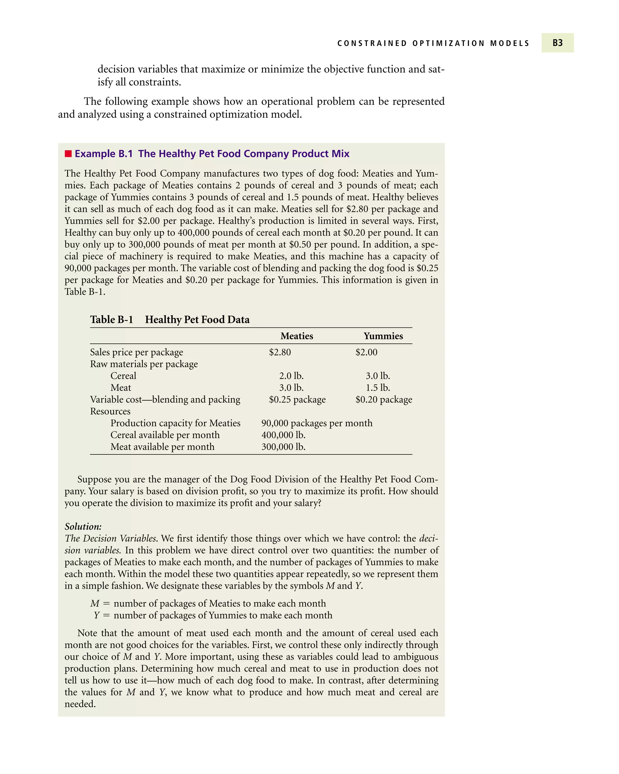
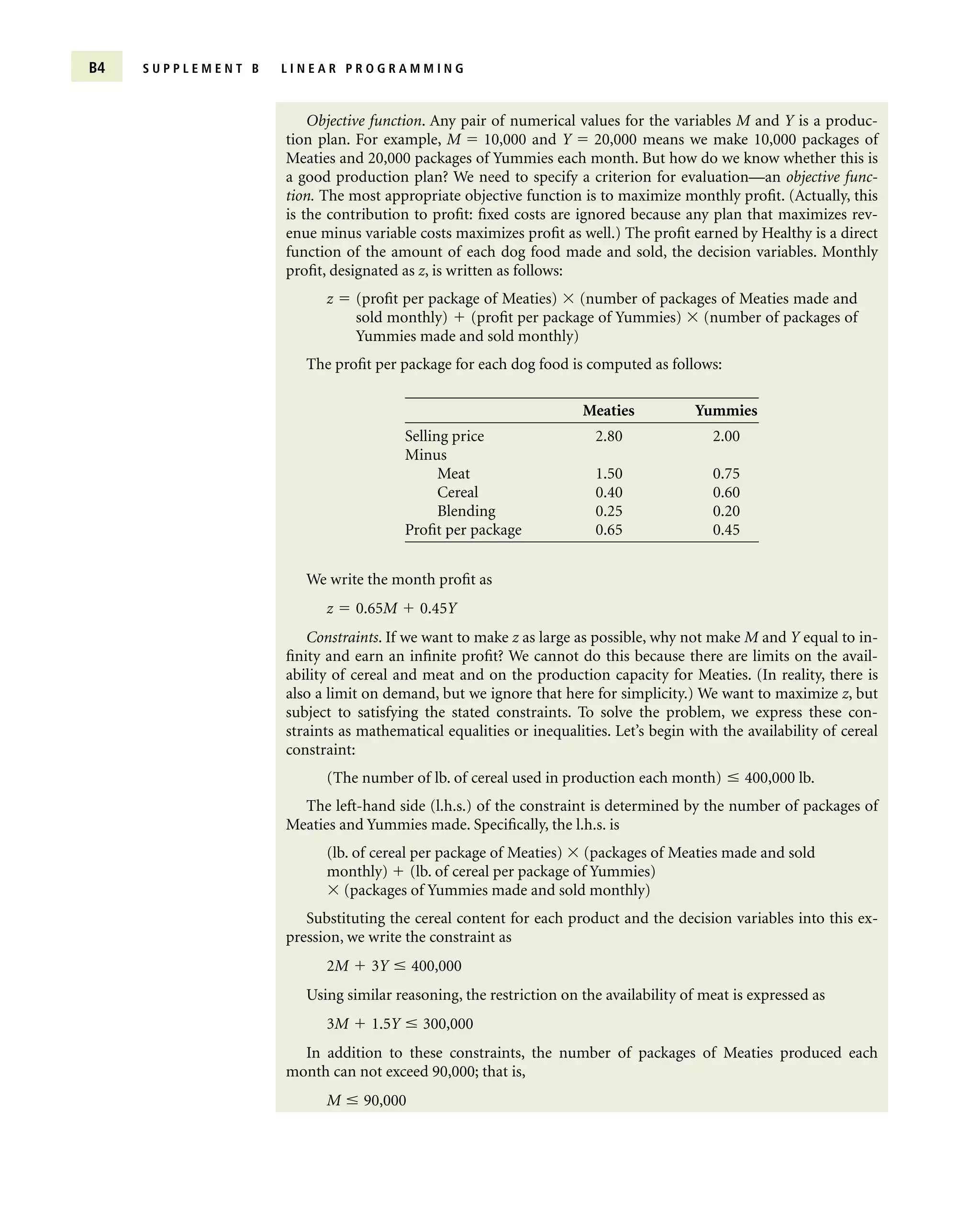
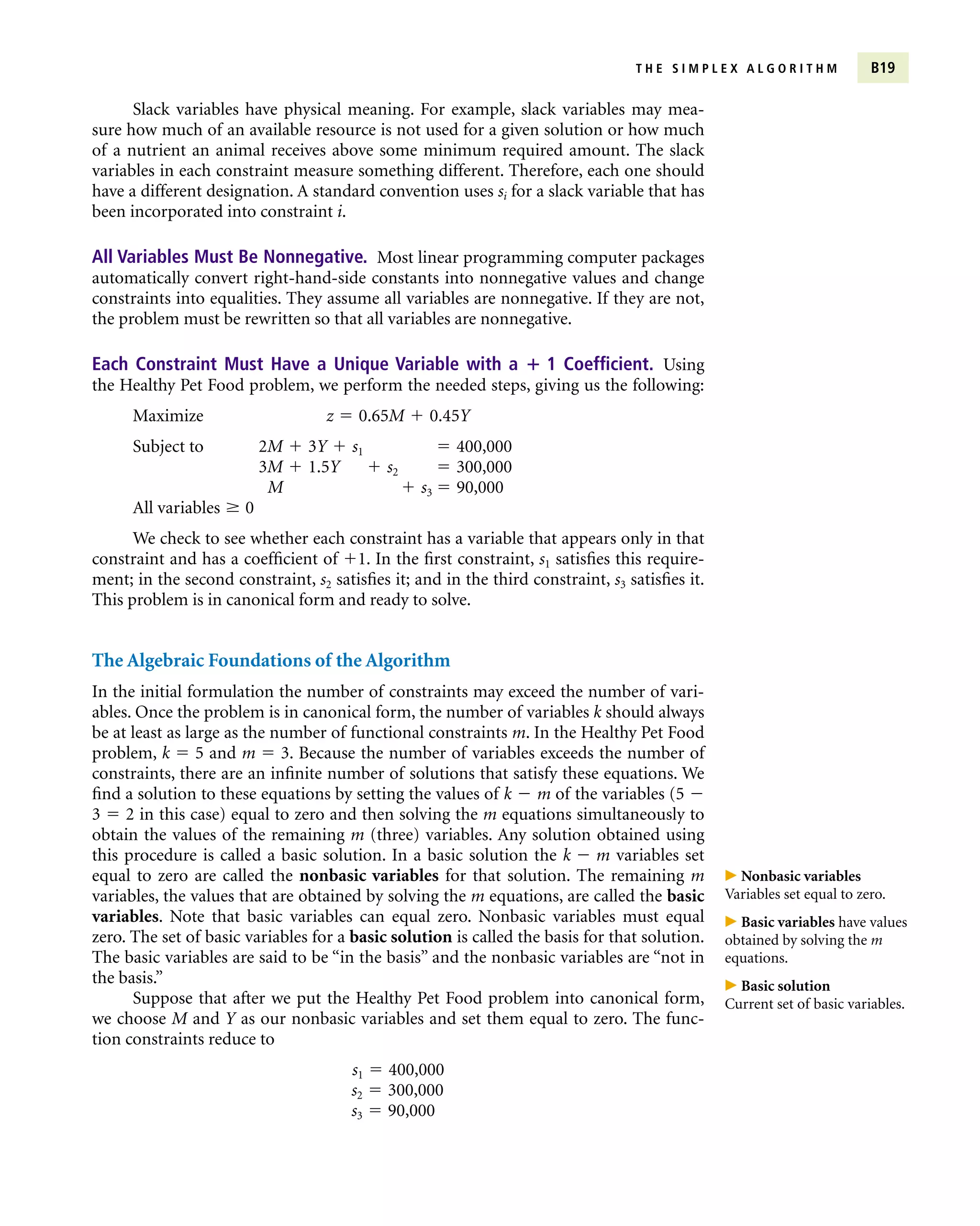
� The Healthy Pet Food Company example models their product mix problem to maximize profit with decision variables for Meaties and Yummies production. The objective is to maximize total profit and constraints include limits on cereal, meat, and Meaties production capacity.
� Optimization models provide benefits like evaluating solutions quickly, structuring the problem, increasing objectivity, and enabling complex problems and "what if" analysis to be addressed. Potential disadvantages include mismodeling the real problem and not considering qualitative factors.
![F O R M U L A T I N G L I N E A R P R O G R A M S B11
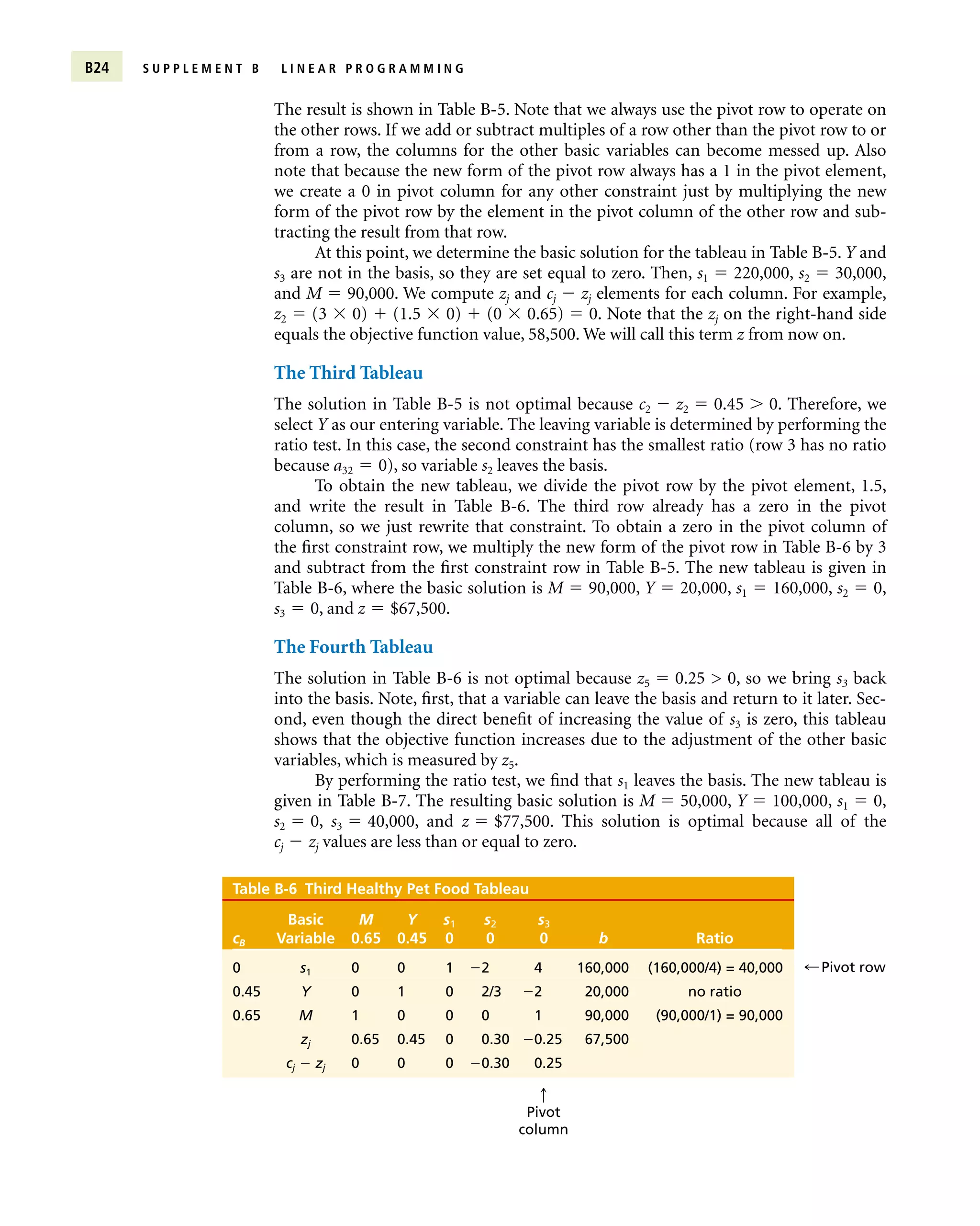
Note that the coefficients for some variables are negative. For example, Solar loses $1.00
on each barrel of raw gas 4 that is blended into premium. Does this imply that the optimal
value for these variables must be zero and that they can be dropped from the problem? No!
In blending operations, it is common for some low-cost materials to be combined with
high-cost materials. Although it appears that we are losing money on the high-cost materi-
als, they make the low-cost materials more valuable, and often the final product cannot be
made without them. For example, tungsten steel combines low-cost iron ore or scrap (worth
$100/ton) with tungsten (costing thousands of dollars per ton) to make steel that might sell
for $500 per ton. The manufacturer loses money on the tungsten (on a per ton basis) but is
more than compensated by the enhanced value of the iron ore. Therefore, we do not omit
variables from the problem unless we can prove that their optimum value is zero.
The next step is to identify the constraints. The availability constraint for each raw gaso-
line is
barrels of raw gas i used per day barrels of gas i available per day
The number of barrels of raw gas i used each day is the amount used to make regular
gasoline xiR plus the amount used each day to make premium gasoline xiP. The availability
constraints can be written as
x1R x1P 20,000
x2R x2P 15,000
x3R x3P 15,000
x4R x4P 10,000
The demand constraints put an upper limit on how much regular and premium gasoline
can be sold. The total amount made of each is the sum of the raw gasolines allocated to
making each gasoline each day. In other words,
x1R x2R x3R x4R 35,000
x1P x2P x3P x4P 23,000
If the model formulation is left at this stage, the optimal solution is to mix the lowest-
cost gasolines into the final products, regardless of octane. Therefore, we need to include
constraints that guarantee the variables will take on values that produce final gasolines with
at least the minimum specified octane ratings. The octane rating of the regular gasoline that
is produced will be a weighted average of the octanes of the raw gasolines used; that is,
octane of regular [86 (barrels of raw gas 1 used/day to make regular)
88 (barrels of raw gas 2 used/day to make regular) 96 (barrels of raw
gas 4 used/day to make regular)]/[total barrels of raw gases blended into regular
gasoline]
which should be at least 89. Substituting the appropriate variable names for these quantities
produces the constraint
[86x1R 88x2R 92x3R 96x4R]/[x1R x2R x3R x4R] 89
Multiplying both sides by (x1R x2R x3R x4R) and then gathering terms so that
variables appear only once and all are on the left-hand side yields
3x1R x2R x3R 7x4R 0
Using the same approach to guarantee an octane of 93 for premium gas produces the
constraint
7x1R 5x2R x3R 3x4R 0
Finally, all variables should be nonnegative in value. The optimal solution to this linear
program is x1R 11,428.57, x2R 9107.14, x3R 14,464.29, x4R 0, x1P 0, x2P
5892.86, x3P 535.71, x4P 10,000, and z $42,142.86 daily.](https://image.slidesharecdn.com/lpexamples-230929221427-aff5f728/75/LP-examples-pdf-11-2048.jpg)
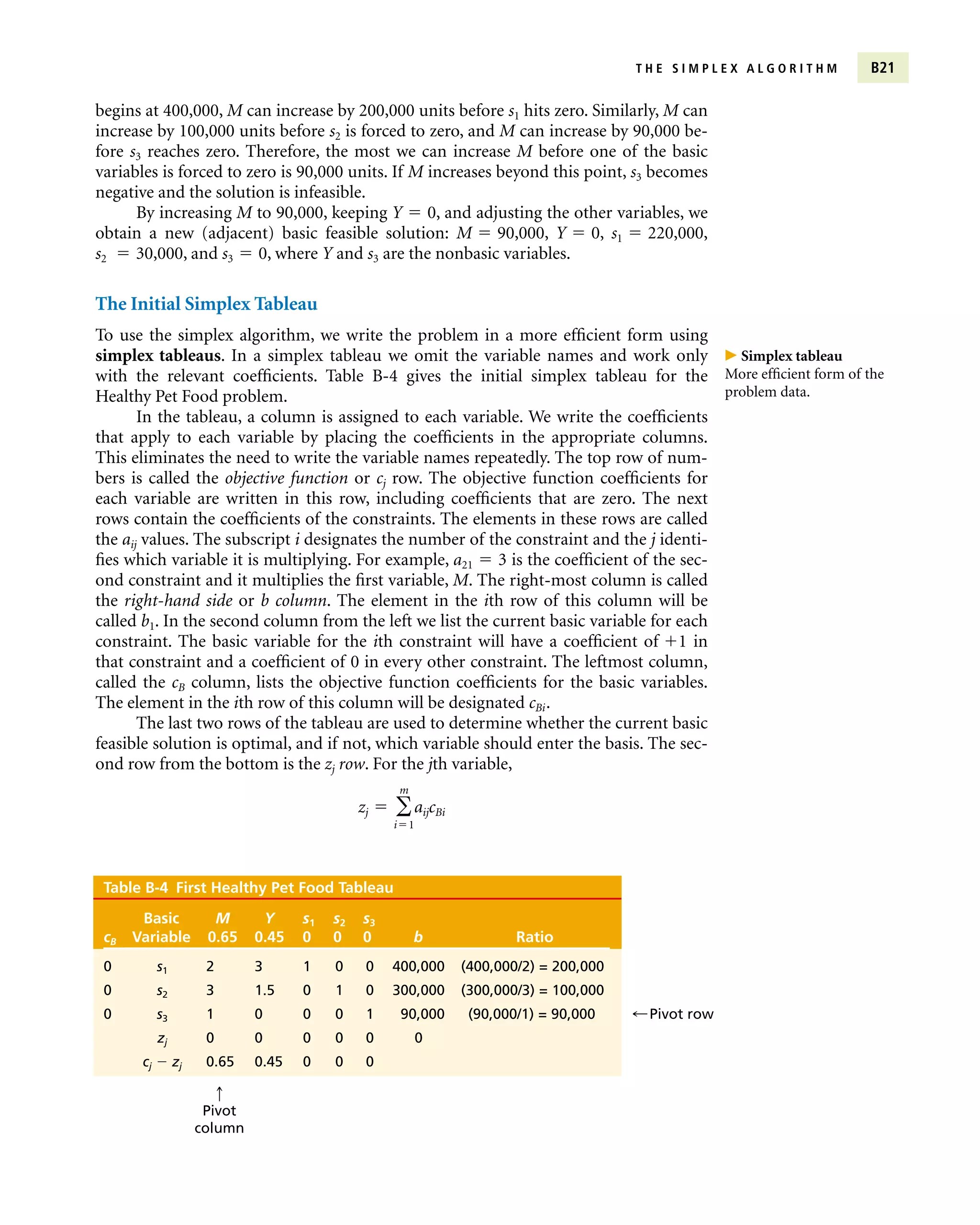
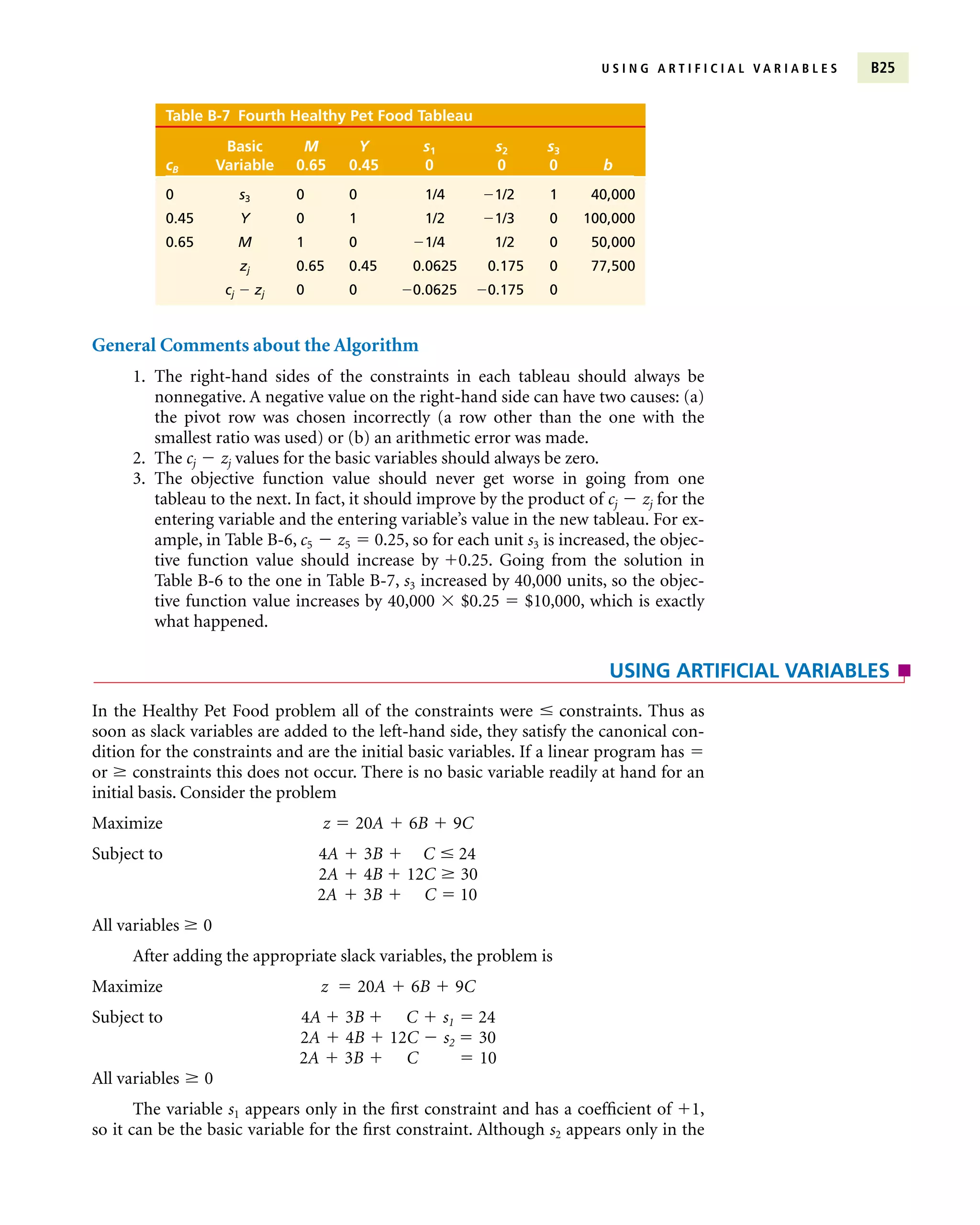
![determined by using a ratio test. For every constraint row i we compute the
ratio bi/ais, if ais 0, where column s is the pivot column. That is, we divide
the right-hand side of each constraint by the element in the pivot column of
the same row, but only if the denominator ais is strictly positive in value. This
ratio computes how much the entering variable can increase in value before
the basic variable in that constraint is forced down to zero. That leaves the
basic variable in the row with the smallest ratio. This row is called the pivot
row. In Table B-4 the ratios for the three constraints are [400,000/2]
200,000, [300,000/3] 100,000, and [90,000/1] 90,000. The smallest ratio
is for the third constraint, so M enters the basis as the variable for the third
constraint and forces s3 out of the basis.
4. Perform pivot operations to obtain the new canonical form. The intersection of
the pivot row and pivot column is called the pivot element. We need to
rewrite the constraints so that they are mathematically equivalent and make
sure that the new basic variable, M, appears in only the third constraint and
has a coefficient of 1. In other words, we want the M column to contain
1 in the pivot element and 0 in every other constraint row. We do this with
row operations. The problem does not change if we multiply any equation by
a nonzero constant, or add or subtract a multiple of any equation to or from
any other equation. We divide the entire pivot row by the value of the pivot
element. In Table B-4, the pivot element is already equal to 1, so the pivot
row does not change. It is just rewritten in Table B-5. If the pivot element
had been 4, we would divide the entire pivot row (except the two leftmost
columns) by 4. The new form of the pivot row is always a multiple of the
current pivot row, so a multiple of this new form of the pivot row can be
added to or subtracted from the other rows.
To obtain a zero in the M column of the first constraint, we multiply the pivot
row (third row) by 2 and subtract from the first constraint row:
[2 3 1 0 0 400,000]
2 [1 0 0 0 1 90,000] [0 3 1 0 2 220,000]
The new form of the first constraint in shown in Table B-5. To obtain a zero in the M
column of the second constraint, multiply the pivot row by 3 and subtract from the
second constraint row:
[3 1.5 0 1 0 300,000]
3 [1 0 0 0 1 90,000] [0 1.5 0 1 3 30,000]
T H E S I M P L E X A L G O R I T H M B23
The ratio test is used to
determine the leaving vari-
able.
Pivot row
The row with smallest ratio.
Pivot element
Intersection of the pivot row
and the pivot column.
Table B-5 Second Healthy Pet Food Tableau
Basic M Y s1 s2 s3
cB Variable 0.65 0.45 0 0 0 b Ratio
0 s1 0 3 1 0 2 220,000 (220,000/3) 73,333
0 s2 0 1.5 0 1 3 30,000 (30,000/1.5) 20,000
0.65 M 1 0 0 0 1 90,000 no ratio
zj 0.65 0 0 0 0.65 58,500
cj zj 0 0.45 0 0 0.65
;Pivot row
q
Pivot
column](https://image.slidesharecdn.com/lpexamples-230929221427-aff5f728/75/LP-examples-pdf-23-2048.jpg)