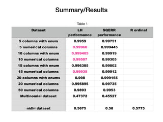
The document discusses logistic ordinal regression, focusing on its application in predicting ordinal variables significant for preference modeling in social sciences. It outlines the methodology for building linear models, updating model parameters, and making predictions, as well as implementing these models using H2O. The results demonstrate the performance of various datasets under different configurations, highlighting the effectiveness of the models.

1. Logistic Ordinal Regression
Wendy C Wong
Michal K and Nidhi M

2. Table of Content
• Ordinal Regression
• Building Linear Models Ordinal Regression
• Linear Models used;
• model parameters updates;
• model predictions
• H2O implementations
• Example and results

3. What is Ordinal Regression?
• Ordinal regression/classification or ranking learning is a
regression analysis used to predict an ordinal variable (a
variable where the relative ordering between different
values is significant);
• Ordinal regression are used most often in social sciences
to model human levels of preference/satisfaction (levels
1-5 for very poor, poor, average, good, excellent)

4. Linear Models used for Ordinal Regression
• Let be our predictor of size p and be the associated
ordinal response. Note: takes value from 1 to K.
• A GLM is used to fit ONE coefficient vector for all classes of
the ordinal variable response and a set of thresholds to a data
set.
• model the CUMULATIVE PROBABILITY as the logistic function
• Note that the separating hyperplanes are parallel for all
classes. The non-decreasing vector is
used to separate all the classes.
• Ordered Probit-standard normal distribution and Proportional
Hazards:
xi
1 + exp(−exp(βT
xi + θj))
yj
θ1 < θ2 < . . . < θK−1
P(y < = j |xi) = σ(βT
xi + θj) = 1/(1 + exp(−βT
xi − θj)) = γij
yi

6. Model Parameters Updates
• The likelihood function:
• The log-likelihood function is
• The pdfs are:
• for j = 1
• for j = K
• To find the model parameters, maximize the log-likelihood
function minus your favorite regularization penalties. Take
the derivatives and update each model parameter with a
learning rate*the derivative for that model parameter…..
N−1
∏
i=0
pd f (yi = yrespi)
N−1
∑
n=0
log(σ(βT
xi + θyj
) − σ(βT
xi + θyj−1))
pd f (yi = 1) = σ(βT
xi + θ1)
pd f (yi = K ) = 1 − pd f (yi = K − 1)

7. Model Predictions
• The log proportional odds is:
• When the proportional odds > 1 (log(.) > 0), it implies that
it is more probable that the data point belongs to class
j or lower than belonging to classes j+1 and beyond.
• This implies that a data point is classified as:
• class K:
• class j (>=1 and <= K-1): and
log(
γij
1 − γij
) =
1
1 + exp(−βT xi − θj)
1 −
1
1 + exp(−βT xi − θj))
= βT
xi + θj
xi
xi
βT
xi + θK−1 > 0
βT
xi + θj > 0 βT
xi + θj+1 < = 0

8. Alternate Model Parameters Optimization
• I decided to modify the model parameters to directly
increase the probability of correct predictions.
• Hence, I will optimize the error function
where
• for correct prediction
• for incorrect prediction
L(β, θ, xi, yrespi) = (βT
xi + θj)2
N−1
∑
i=0
L(β, θ, xi, yrespi)
L(β, θ, xi, yrespi) = 0
βT
xi + θj < = 0
j < yrespiβT
xi + θj > 0
j > = yrespi
βT
xi + θj > 0
j < yrespi
βT
xi + θj < = 0
j > = yrespi

9. H2O Implementation
• To use ordinal regression, set family=“ordinal”;
• To change model parameters using the likelihood function, do not set solver or
set solver to “GRADIENT_DESCENT_LH”
• To change model parameters using the other loss function, set solver to
“GRADIENT_DESCENT_SQERR”
• Gradient descent: first-order method, use gridsearch to find good learning rate,
regularization values (beta, alpha)….
• In R: ordinal.fit <- h2o.glm(y=Y, x=X, training_frame=
Dtrain, family="ordinal",
solver="GRADIENT_DESCENT_SQERR")
• In Python:
ordinal_fit = H2OGeneralizedLinearEstimator(family="ordinal",
solver=“GRADIENT_DESCENT_LH”)
ordinal_fit.train(y=Y, x=X, training_frame=Dtrain)

10. Summary/Results
Table 1
Dataset LH
performance
SQERR
performance
R ordinal
5 columns with enum 0.9959 0.99751
5 numerical columns 0.99968 0.999445
10 columns with enum 0.999405 0.99919
10 numerical columns 0.99507 0.99305
15 columns with enum 0.996385 0.99802
15 numerical columns 0.99938 0.99912
20 columns with enums 0.998 0.999155
20 numerical columns 0.995895 0.99735
50 numerical columns 0.9893 0.9953
Multinomial dataset 0.47372 0.45527
nidhi dataset 0.5675 0.58 0.5775

11. Reference
• Peter McCullagh, Regression Models for Ordinal Data, J.
R. Statist, Soc. B(1980), 42, No 2, pp.109-142
• Wikipedia, Ordinal Regression
• Alan Agresti, “Analysis of Ordinal Categorical data”, John
Wiley & Sons, Inc. July, 2012