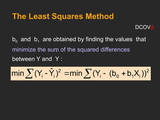
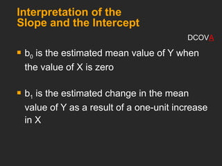
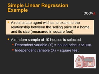
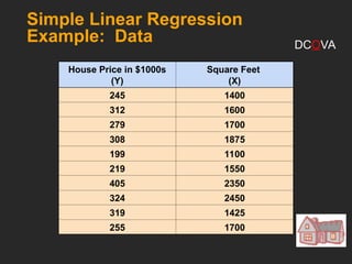
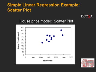
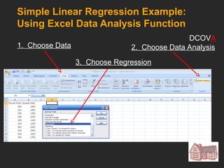
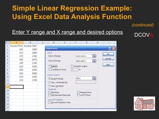
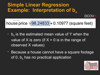
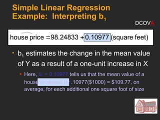
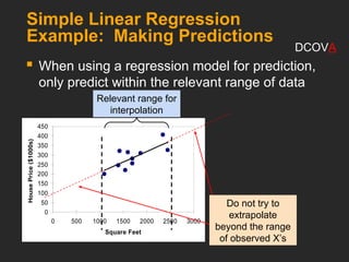
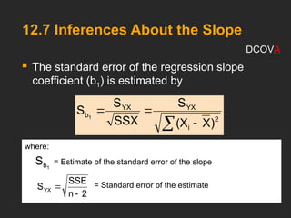
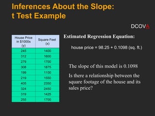
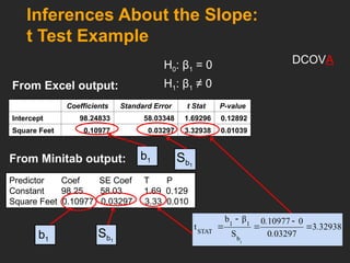
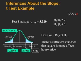
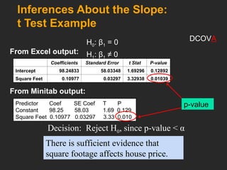
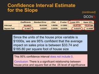
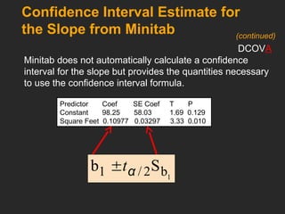
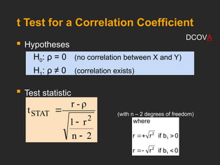
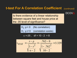
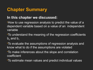
Simple Linear
Regression
Objectives
In this chapter, you learn:
How to use regression analysis to predict the value of a
dependent variable based on a value of an independent
variable
To understand the meaning of the regression coefficients
b0 and b1
To evaluate the assumptions of regression analysis and
know what to do if the assumptions are violated
To make inferences about the slope and correlation
coefficient
To estimate mean values and predict individual values
Correlation vs. Regression
 A scatter plot can be used to show the
relationship between two variables
 Correlation analysis is used to measure the
strength of the association (linear relationship)
between two variables
 Correlation is only concerned with strength of the
relationship
 No causal effect is implied with correlation
 Scatter plots were first presented in Ch. 2
 Correlation was first presented in Ch. 3
DCOVA
12.1 Regression Models
Y
X
Y
X
Y
Y
X
X
Linear relationships Curvilinear relationships
DCOVA
Types of Relationships
Y
X
Y
X
Y
Y
X
X
Strong relationships Weak relationships
(continued)
DCOVA
Types of Relationships
Y
X
Y
X
No relationship
DCOVA
(continued)
12.2 Introduction to
Regression Analysis
 Regression analysis is used to:
 Predict the value of a dependent variable based on
the value of at least one independent variable
 Explain the impact of changes in an independent
variable on the dependent variable
 Dependent variable: the variable we wish to
predict or explain
 Independent variable: the variable used to
predict or explain the
dependent variable
DCOVA
Simple Linear Regression Model
 Only one independent variable, X
 Relationship between X and Y is described by
a linear function
 Changes in Y are assumed to be related to
changes in X
DCOVA
i
i
1
0
i ε
X
β
β
Y 


Linear component
Simple Linear Regression Model
Population
Y intercept
Population
Slope
Coefficient
Random
Error
term
Dependent
Variable
Independent
Variable
Random Error
component
DCOVA
Random Error
for this Xi value
Y
X
Observed Value
of Y for Xi
Predicted Value
of Y for Xi
i
i
1
0
i ε
X
β
β
Y 


Xi
Slope = β1
Intercept = β0
εi
Simple Linear Regression
Model DCOVA
(continued)
Simple Linear Regression Equation
(Prediction Line)
i
1
0
i X
b
b
Ŷ 

The simple linear regression equation provides an
estimate of the population regression line
Estimate of
the regression
intercept
Estimate of the
regression slope
Estimated
(or predicted)
Y value for
observation i
Value of X for
observation i
DCOVA
The Least Squares Method
b0 and b1 are obtained by finding the values that
minimize the sum of the squared differences
between Y and Y :
2
i
1
0
i
2
i
i ))
X
b
(b
(Y
min
)
Ŷ
(Y
min 


 

DCOVA

Finding the Least Squares
Equation
 The coefficients b0 and b1, and other
regression results in this chapter, will be
found using Excel or Minitab
Formulas are shown in the text for those
who are interested
DCOVA
Interpretation of the
Slope and the Intercept
 b0 is the estimated mean value of Y when
the value of X is zero
 b1 is the estimated change in the mean
value of Y as a result of a one-unit increase
in X
DCOVA
Simple Linear Regression
Example
 A real estate agent wishes to examine the
relationship between the selling price of a home
and its size (measured in square feet)
 A random sample of 10 houses is selected
 Dependent variable (Y) = house price in $1000s
 Independent variable (X) = square feet
DCOVA
Simple Linear Regression
Example: Data
House Price in $1000s
(Y)
Square Feet
(X)
245 1400
312 1600
279 1700
308 1875
199 1100
219 1550
405 2350
324 2450
319 1425
255 1700
DCOVA
0
50
100
150
200
250
300
350
400
450
0 500 1000 1500 2000 2500 3000
House
Price
($1000s)
Square Feet
Simple Linear Regression Example:
Scatter Plot
House price model: Scatter Plot
DCOVA
Simple Linear Regression Example:
Using Excel Data Analysis Function
1. Choose Data 2. Choose Data Analysis
3. Choose Regression
DCOVA
Simple Linear Regression Example:
Using Excel Data Analysis Function
Enter Y range and X range and desired options
DCOVA
(continued)
Simple Linear Regression
Example: Using PHStat
Add-Ins: PHStat: Regression: Simple Linear Regression
Simple Linear Regression Example:
Excel Output
Regression Statistics
Multiple R 0.76211
R Square 0.58082
Adjusted R Square 0.52842
Standard Error 41.33032
Observations 10
ANOVA
df SS MS F Significance F
Regression 1 18934.9348 18934.9348 11.0848 0.01039
Residual 8 13665.5652 1708.1957
Total 9 32600.5000
Coefficients Standard Error t Stat P-value Lower 95% Upper 95%
Intercept 98.24833 58.03348 1.69296 0.12892 -35.57720 232.07386
Square Feet 0.10977 0.03297 3.32938 0.01039 0.03374 0.18580
The regression equation is:
feet)
(square
0.10977
98.24833
price
house 

DCOVA
Simple Linear Regression Example:
Minitab Output
The regression equation is
Price = 98.2 + 0.110 Square Feet
Predictor Coef SE Coef T P
Constant 98.25 58.03 1.69 0.129
Square Feet 0.10977 0.03297 3.33 0.010
S = 41.3303 R-Sq = 58.1% R-Sq(adj) = 52.8%
Analysis of Variance
Source DF SS MS F P
Regression 1 18935 18935 11.08 0.010
Residual Error 8 13666 1708
Total 9 32600
The regression
equation is:
house price = 98.24833 +
0.10977 (square feet)
DCOVA
0
50
100
150
200
250
300
350
400
450
0 500 1000 1500 2000 2500 3000
Square Feet
House
Price
($1000s)
Simple Linear Regression Example:
Graphical Representation
House price model: Scatter Plot and Prediction Line
feet)
(square
0.10977
98.24833
price
house 

Slope
= 0.10977
Intercept
= 98.248
DCOVA
Simple Linear Regression
Example: Interpretation of bo
 b0 is the estimated mean value of Y when the
value of X is zero (if X = 0 is in the range of
observed X values)
 Because a house cannot have a square footage
of 0, b0 has no practical application
feet)
(square
0.10977
98.24833
price
house 

DCOVA
Simple Linear Regression
Example: Interpreting b1
 b1 estimates the change in the mean value
of Y as a result of a one-unit increase in X
 Here, b1 = 0.10977 tells us that the mean value of a
house increases by .10977($1000) = $109.77, on
average, for each additional one square foot of size
feet)
(square
0.10977
98.24833
price
house 

DCOVA
317.85
0)
0.1098(200
98.25
(sq.ft.)
0.1098
98.25
price
house





Predict the price for a house
with 2000 square feet:
The predicted price for a house with 2000
square feet is 317.85($1,000s) = $317,850
Simple Linear Regression
Example: Making Predictions
DCOVA
0
50
100
150
200
250
300
350
400
450
0 500 1000 1500 2000 2500 3000
Square Feet
House
Price
($1000s)
Simple Linear Regression
Example: Making Predictions
 When using a regression model for prediction,
only predict within the relevant range of data
Relevant range for
interpolation
Do not try to
extrapolate
beyond the range
of observed X’s
DCOVA
12.4 Assumptions of Regression
L.I.N.E
 Linearity
 The relationship between X and Y is linear
 Independence of Errors
 Error values are statistically independent
 Particularly important when data are collected over a period
of time
 Normality of Error
 Error values are normally distributed for any given value of X
 Equal Variance (also called homoscedasticity)
 The probability distribution of the errors has constant
variance
DCOVA
12.7 Inferences About the Slope
 The standard error of the regression slope
coefficient (b1) is estimated by
 


2
i
YX
YX
b
)
X
(X
S
SSX
S
S 1
where:
= Estimate of the standard error of the slope
= Standard error of the estimate
1
b
S
2
n
SSE
SYX


DCOVA
Inferences About the Slope:
t Test
 t test for a population slope
 Is there a linear relationship between X and Y?
 Null and alternative hypotheses

H0: β1 = 0 (no linear relationship)

H1: β1 ≠ 0 (linear relationship does exist)
 Test statistic
1
b
1
1
STAT
S
β
b
t


2
n
d.f. 

where:
b1 = regression slope
coefficient
β1 = hypothesized slope
Sb1 = standard
error of the slope
DCOVA
Inferences About the Slope:
t Test Example
House Price
in $1000s
(y)
Square Feet
(x)
245 1400
312 1600
279 1700
308 1875
199 1100
219 1550
405 2350
324 2450
319 1425
255 1700
Estimated Regression Equation:
The slope of this model is 0.1098
Is there a relationship between the
square footage of the house and its
sales price?
DCOVA
house price = 98.25 + 0.1098 (sq. ft.)
Inferences About the Slope:
t Test Example
1
b
S
H0: β1 = 0
H1: β1 ≠ 0
From Excel output:
Coefficients Standard Error t Stat P-value
Intercept 98.24833 58.03348 1.69296 0.12892
Square Feet 0.10977 0.03297 3.32938 0.01039
1
b
S
b1
32938
3
03297
0
0
10977
0
S
β
b
t
1
b
1
1
STAT
.
.
.





Predictor Coef SE Coef T P
Constant 98.25 58.03 1.69 0.129
Square Feet 0.10977 0.03297 3.33 0.010
From Minitab output:
b1
DCOVA
Inferences About the Slope:
t Test Example
H0: β1 = 0
H1: β1 ≠ 0
Test Statistic: tSTAT = 3.329
There is sufficient evidence
that square footage affects
house price
Decision: Reject H0
Reject H0
Reject H0
/2=.025
-tα/2
Do not reject H0
0
tα/2
/2=.025
-2.3060 2.3060 3.329
d.f. = 10- 2 = 8
DCOVA
Inferences About the Slope:
t Test Example
H0: β1 = 0
H1: β1 ≠ 0
From Excel output:
Coefficients Standard Error t Stat P-value
Intercept 98.24833 58.03348 1.69296 0.12892
Square Feet 0.10977 0.03297 3.32938 0.01039
p-value
There is sufficient evidence that
square footage affects house price.
Decision: Reject H0, since p-value < α
Predictor Coef SE Coef T P
Constant 98.25 58.03 1.69 0.129
Square Feet 0.10977 0.03297 3.33 0.010
From Minitab output:
DCOVA
F Test for Significance
 F Test statistic:
where
MSE
MSR
FSTAT 
1
k
n
SSE
MSE
k
SSR
MSR




where FSTAT follows an F distribution with k numerator and (n – k - 1)
denominator degrees of freedom
(k = the number of independent variables in the regression model)
DCOVA
Regression Statistics
Multiple R 0.76211
R Square 0.58082
Adjusted R Square 0.52842
Standard Error 41.33032
Observations 10
ANOVA
df SS MS F Significance F
Regression 1 18934.9348 18934.9348 11.0848 0.01039
Residual 8 13665.5652 1708.1957
Total 9 32600.5000
F-Test for Significance
Excel Output
11.0848
1708.1957
18934.9348
MSE
MSR
FSTAT 


With 1 and 8 degrees
of freedom
p-value for
the F-Test
DCOVA
F-Test for Significance
Minitab Output
11.0848
1708.1957
18934.9348
MSE
MSR
FSTAT 


Analysis of Variance
Source DF SS MS F P
Regression 1 18935 18935 11.08 0.010
Residual Error 8 13666 1708
Total 9 32600
With 1 and 8 degrees
of freedom
p-value for
the F-Test
DCOVA
F Test for Significance
H0: β1 = 0
H1: β1 ≠ 0
 = .05
df1= 1 df2 = 8
Test Statistic:
Decision:
Conclusion:
Reject H0 at  = 0.05
There is sufficient evidence that
house size affects selling price
0
 = .05
F.05 = 5.32
Reject H0
Do not
reject H0
11.08
FSTAT 

MSE
MSR
Critical
Value:
F = 5.32
F
DCOVA
(continued)
Confidence Interval Estimate
for the Slope
Confidence Interval Estimate of the Slope:
Excel Printout for House Prices:
At 95% level of confidence, the confidence interval for
the slope is (0.0337, 0.1858)
1
b
2
/
1 S
b α
t

Coefficients Standard Error t Stat P-value Lower 95% Upper 95%
Intercept 98.24833 58.03348 1.69296 0.12892 -35.57720 232.07386
Square Feet 0.10977 0.03297 3.32938 0.01039 0.03374 0.18580
d.f. = n - 2
DCOVA
Since the units of the house price variable is
$1000s, we are 95% confident that the average
impact on sales price is between $33.74 and
$185.80 per square foot of house size
Coefficients Standard Error t Stat P-value Lower 95% Upper 95%
Intercept 98.24833 58.03348 1.69296 0.12892 -35.57720 232.07386
Square Feet 0.10977 0.03297 3.32938 0.01039 0.03374 0.18580
This 95% confidence interval does not include 0.
Conclusion: There is a significant relationship between
house price and square feet at the .05 level of significance
Confidence Interval Estimate
for the Slope
DCOVA
(continued)
Confidence Interval Estimate for
the Slope from Minitab
DCOVA
Predictor Coef SE Coef T P
Constant 98.25 58.03 1.69 0.129
Square Feet 0.10977 0.03297 3.33 0.010
Minitab does not automatically calculate a confidence
interval for the slope but provides the quantities necessary
to use the confidence interval formula.
1
b
2
/
1 S
b α
t

(continued)
t Test for a Correlation Coefficient
 Hypotheses
H0: ρ = 0 (no correlation between X and Y)
H1: ρ ≠ 0 (correlation exists)

Test statistic
(with n – 2 degrees of freedom)
2
n
r
1
ρ
-
r
t
2
STAT



0
b
if
r
r
0
b
if
r
r
where
1
2
1
2






DCOVA
t-test For A Correlation Coefficient
Is there evidence of a linear relationship
between square feet and house price at
the .05 level of significance?
H0: ρ = 0 (No correlation)
H1: ρ ≠ 0 (correlation exists)
 =.05 , df = 10 - 2 = 8
3.329
2
10
.762
1
0
.762
2
n
r
1
ρ
r
t
2
2
STAT 








DCOVA
(continued)
t-test For A Correlation Coefficient
Conclusion:
There is
evidence of a
linear association
at the 5% level of
significance
Decision:
Reject H0
Reject H0
Reject H0
/2=.025
-tα/2
Do not reject H0
0
tα/2
/2=.025
-2.3060 2.3060
3.329
d.f. = 10-2 = 8
3.329
2
10
.762
1
0
.762
2
n
r
1
ρ
r
t
2
2
STAT 








DCOVA
(continued)
Chapter Summary
In this chapter we discussed:
How to use regression analysis to predict the value of a
dependent variable based on a value of an independent
variable
To understand the meaning of the regression coefficients
b0 and b1
To evaluate the assumptions of regression analysis and
know what to do if the assumptions are violated
To make inferences about the slope and correlation
coefficient
To estimate mean values and predict individual values

Linear Regression statistical analysis s

  • 1.
  • 2.
    Objectives In this chapter,you learn: How to use regression analysis to predict the value of a dependent variable based on a value of an independent variable To understand the meaning of the regression coefficients b0 and b1 To evaluate the assumptions of regression analysis and know what to do if the assumptions are violated To make inferences about the slope and correlation coefficient To estimate mean values and predict individual values
  • 3.
    Correlation vs. Regression A scatter plot can be used to show the relationship between two variables  Correlation analysis is used to measure the strength of the association (linear relationship) between two variables  Correlation is only concerned with strength of the relationship  No causal effect is implied with correlation  Scatter plots were first presented in Ch. 2  Correlation was first presented in Ch. 3 DCOVA
  • 4.
    12.1 Regression Models Y X Y X Y Y X X Linearrelationships Curvilinear relationships DCOVA
  • 5.
    Types of Relationships Y X Y X Y Y X X Strongrelationships Weak relationships (continued) DCOVA
  • 6.
    Types of Relationships Y X Y X Norelationship DCOVA (continued)
  • 7.
    12.2 Introduction to RegressionAnalysis  Regression analysis is used to:  Predict the value of a dependent variable based on the value of at least one independent variable  Explain the impact of changes in an independent variable on the dependent variable  Dependent variable: the variable we wish to predict or explain  Independent variable: the variable used to predict or explain the dependent variable DCOVA
  • 8.
    Simple Linear RegressionModel  Only one independent variable, X  Relationship between X and Y is described by a linear function  Changes in Y are assumed to be related to changes in X DCOVA
  • 9.
    i i 1 0 i ε X β β Y    Linearcomponent Simple Linear Regression Model Population Y intercept Population Slope Coefficient Random Error term Dependent Variable Independent Variable Random Error component DCOVA
  • 10.
    Random Error for thisXi value Y X Observed Value of Y for Xi Predicted Value of Y for Xi i i 1 0 i ε X β β Y    Xi Slope = β1 Intercept = β0 εi Simple Linear Regression Model DCOVA (continued)
  • 11.
    Simple Linear RegressionEquation (Prediction Line) i 1 0 i X b b Ŷ   The simple linear regression equation provides an estimate of the population regression line Estimate of the regression intercept Estimate of the regression slope Estimated (or predicted) Y value for observation i Value of X for observation i DCOVA
  • 12.
    The Least SquaresMethod b0 and b1 are obtained by finding the values that minimize the sum of the squared differences between Y and Y : 2 i 1 0 i 2 i i )) X b (b (Y min ) Ŷ (Y min       DCOVA 
  • 13.
    Finding the LeastSquares Equation  The coefficients b0 and b1, and other regression results in this chapter, will be found using Excel or Minitab Formulas are shown in the text for those who are interested DCOVA
  • 14.
    Interpretation of the Slopeand the Intercept  b0 is the estimated mean value of Y when the value of X is zero  b1 is the estimated change in the mean value of Y as a result of a one-unit increase in X DCOVA
  • 15.
    Simple Linear Regression Example A real estate agent wishes to examine the relationship between the selling price of a home and its size (measured in square feet)  A random sample of 10 houses is selected  Dependent variable (Y) = house price in $1000s  Independent variable (X) = square feet DCOVA
  • 16.
    Simple Linear Regression Example:Data House Price in $1000s (Y) Square Feet (X) 245 1400 312 1600 279 1700 308 1875 199 1100 219 1550 405 2350 324 2450 319 1425 255 1700 DCOVA
  • 17.
    0 50 100 150 200 250 300 350 400 450 0 500 10001500 2000 2500 3000 House Price ($1000s) Square Feet Simple Linear Regression Example: Scatter Plot House price model: Scatter Plot DCOVA
  • 18.
    Simple Linear RegressionExample: Using Excel Data Analysis Function 1. Choose Data 2. Choose Data Analysis 3. Choose Regression DCOVA
  • 19.
    Simple Linear RegressionExample: Using Excel Data Analysis Function Enter Y range and X range and desired options DCOVA (continued)
  • 20.
    Simple Linear Regression Example:Using PHStat Add-Ins: PHStat: Regression: Simple Linear Regression
  • 21.
    Simple Linear RegressionExample: Excel Output Regression Statistics Multiple R 0.76211 R Square 0.58082 Adjusted R Square 0.52842 Standard Error 41.33032 Observations 10 ANOVA df SS MS F Significance F Regression 1 18934.9348 18934.9348 11.0848 0.01039 Residual 8 13665.5652 1708.1957 Total 9 32600.5000 Coefficients Standard Error t Stat P-value Lower 95% Upper 95% Intercept 98.24833 58.03348 1.69296 0.12892 -35.57720 232.07386 Square Feet 0.10977 0.03297 3.32938 0.01039 0.03374 0.18580 The regression equation is: feet) (square 0.10977 98.24833 price house   DCOVA
  • 22.
    Simple Linear RegressionExample: Minitab Output The regression equation is Price = 98.2 + 0.110 Square Feet Predictor Coef SE Coef T P Constant 98.25 58.03 1.69 0.129 Square Feet 0.10977 0.03297 3.33 0.010 S = 41.3303 R-Sq = 58.1% R-Sq(adj) = 52.8% Analysis of Variance Source DF SS MS F P Regression 1 18935 18935 11.08 0.010 Residual Error 8 13666 1708 Total 9 32600 The regression equation is: house price = 98.24833 + 0.10977 (square feet) DCOVA
  • 23.
    0 50 100 150 200 250 300 350 400 450 0 500 10001500 2000 2500 3000 Square Feet House Price ($1000s) Simple Linear Regression Example: Graphical Representation House price model: Scatter Plot and Prediction Line feet) (square 0.10977 98.24833 price house   Slope = 0.10977 Intercept = 98.248 DCOVA
  • 24.
    Simple Linear Regression Example:Interpretation of bo  b0 is the estimated mean value of Y when the value of X is zero (if X = 0 is in the range of observed X values)  Because a house cannot have a square footage of 0, b0 has no practical application feet) (square 0.10977 98.24833 price house   DCOVA
  • 25.
    Simple Linear Regression Example:Interpreting b1  b1 estimates the change in the mean value of Y as a result of a one-unit increase in X  Here, b1 = 0.10977 tells us that the mean value of a house increases by .10977($1000) = $109.77, on average, for each additional one square foot of size feet) (square 0.10977 98.24833 price house   DCOVA
  • 26.
    317.85 0) 0.1098(200 98.25 (sq.ft.) 0.1098 98.25 price house      Predict the pricefor a house with 2000 square feet: The predicted price for a house with 2000 square feet is 317.85($1,000s) = $317,850 Simple Linear Regression Example: Making Predictions DCOVA
  • 27.
    0 50 100 150 200 250 300 350 400 450 0 500 10001500 2000 2500 3000 Square Feet House Price ($1000s) Simple Linear Regression Example: Making Predictions  When using a regression model for prediction, only predict within the relevant range of data Relevant range for interpolation Do not try to extrapolate beyond the range of observed X’s DCOVA
  • 28.
    12.4 Assumptions ofRegression L.I.N.E  Linearity  The relationship between X and Y is linear  Independence of Errors  Error values are statistically independent  Particularly important when data are collected over a period of time  Normality of Error  Error values are normally distributed for any given value of X  Equal Variance (also called homoscedasticity)  The probability distribution of the errors has constant variance DCOVA
  • 29.
    12.7 Inferences Aboutthe Slope  The standard error of the regression slope coefficient (b1) is estimated by     2 i YX YX b ) X (X S SSX S S 1 where: = Estimate of the standard error of the slope = Standard error of the estimate 1 b S 2 n SSE SYX   DCOVA
  • 30.
    Inferences About theSlope: t Test  t test for a population slope  Is there a linear relationship between X and Y?  Null and alternative hypotheses  H0: β1 = 0 (no linear relationship)  H1: β1 ≠ 0 (linear relationship does exist)  Test statistic 1 b 1 1 STAT S β b t   2 n d.f.   where: b1 = regression slope coefficient β1 = hypothesized slope Sb1 = standard error of the slope DCOVA
  • 31.
    Inferences About theSlope: t Test Example House Price in $1000s (y) Square Feet (x) 245 1400 312 1600 279 1700 308 1875 199 1100 219 1550 405 2350 324 2450 319 1425 255 1700 Estimated Regression Equation: The slope of this model is 0.1098 Is there a relationship between the square footage of the house and its sales price? DCOVA house price = 98.25 + 0.1098 (sq. ft.)
  • 32.
    Inferences About theSlope: t Test Example 1 b S H0: β1 = 0 H1: β1 ≠ 0 From Excel output: Coefficients Standard Error t Stat P-value Intercept 98.24833 58.03348 1.69296 0.12892 Square Feet 0.10977 0.03297 3.32938 0.01039 1 b S b1 32938 3 03297 0 0 10977 0 S β b t 1 b 1 1 STAT . . .      Predictor Coef SE Coef T P Constant 98.25 58.03 1.69 0.129 Square Feet 0.10977 0.03297 3.33 0.010 From Minitab output: b1 DCOVA
  • 33.
    Inferences About theSlope: t Test Example H0: β1 = 0 H1: β1 ≠ 0 Test Statistic: tSTAT = 3.329 There is sufficient evidence that square footage affects house price Decision: Reject H0 Reject H0 Reject H0 /2=.025 -tα/2 Do not reject H0 0 tα/2 /2=.025 -2.3060 2.3060 3.329 d.f. = 10- 2 = 8 DCOVA
  • 34.
    Inferences About theSlope: t Test Example H0: β1 = 0 H1: β1 ≠ 0 From Excel output: Coefficients Standard Error t Stat P-value Intercept 98.24833 58.03348 1.69296 0.12892 Square Feet 0.10977 0.03297 3.32938 0.01039 p-value There is sufficient evidence that square footage affects house price. Decision: Reject H0, since p-value < α Predictor Coef SE Coef T P Constant 98.25 58.03 1.69 0.129 Square Feet 0.10977 0.03297 3.33 0.010 From Minitab output: DCOVA
  • 35.
    F Test forSignificance  F Test statistic: where MSE MSR FSTAT  1 k n SSE MSE k SSR MSR     where FSTAT follows an F distribution with k numerator and (n – k - 1) denominator degrees of freedom (k = the number of independent variables in the regression model) DCOVA
  • 36.
    Regression Statistics Multiple R0.76211 R Square 0.58082 Adjusted R Square 0.52842 Standard Error 41.33032 Observations 10 ANOVA df SS MS F Significance F Regression 1 18934.9348 18934.9348 11.0848 0.01039 Residual 8 13665.5652 1708.1957 Total 9 32600.5000 F-Test for Significance Excel Output 11.0848 1708.1957 18934.9348 MSE MSR FSTAT    With 1 and 8 degrees of freedom p-value for the F-Test DCOVA
  • 37.
    F-Test for Significance MinitabOutput 11.0848 1708.1957 18934.9348 MSE MSR FSTAT    Analysis of Variance Source DF SS MS F P Regression 1 18935 18935 11.08 0.010 Residual Error 8 13666 1708 Total 9 32600 With 1 and 8 degrees of freedom p-value for the F-Test DCOVA
  • 38.
    F Test forSignificance H0: β1 = 0 H1: β1 ≠ 0  = .05 df1= 1 df2 = 8 Test Statistic: Decision: Conclusion: Reject H0 at  = 0.05 There is sufficient evidence that house size affects selling price 0  = .05 F.05 = 5.32 Reject H0 Do not reject H0 11.08 FSTAT   MSE MSR Critical Value: F = 5.32 F DCOVA (continued)
  • 39.
    Confidence Interval Estimate forthe Slope Confidence Interval Estimate of the Slope: Excel Printout for House Prices: At 95% level of confidence, the confidence interval for the slope is (0.0337, 0.1858) 1 b 2 / 1 S b α t  Coefficients Standard Error t Stat P-value Lower 95% Upper 95% Intercept 98.24833 58.03348 1.69296 0.12892 -35.57720 232.07386 Square Feet 0.10977 0.03297 3.32938 0.01039 0.03374 0.18580 d.f. = n - 2 DCOVA
  • 40.
    Since the unitsof the house price variable is $1000s, we are 95% confident that the average impact on sales price is between $33.74 and $185.80 per square foot of house size Coefficients Standard Error t Stat P-value Lower 95% Upper 95% Intercept 98.24833 58.03348 1.69296 0.12892 -35.57720 232.07386 Square Feet 0.10977 0.03297 3.32938 0.01039 0.03374 0.18580 This 95% confidence interval does not include 0. Conclusion: There is a significant relationship between house price and square feet at the .05 level of significance Confidence Interval Estimate for the Slope DCOVA (continued)
  • 41.
    Confidence Interval Estimatefor the Slope from Minitab DCOVA Predictor Coef SE Coef T P Constant 98.25 58.03 1.69 0.129 Square Feet 0.10977 0.03297 3.33 0.010 Minitab does not automatically calculate a confidence interval for the slope but provides the quantities necessary to use the confidence interval formula. 1 b 2 / 1 S b α t  (continued)
  • 42.
    t Test fora Correlation Coefficient  Hypotheses H0: ρ = 0 (no correlation between X and Y) H1: ρ ≠ 0 (correlation exists)  Test statistic (with n – 2 degrees of freedom) 2 n r 1 ρ - r t 2 STAT    0 b if r r 0 b if r r where 1 2 1 2       DCOVA
  • 43.
    t-test For ACorrelation Coefficient Is there evidence of a linear relationship between square feet and house price at the .05 level of significance? H0: ρ = 0 (No correlation) H1: ρ ≠ 0 (correlation exists)  =.05 , df = 10 - 2 = 8 3.329 2 10 .762 1 0 .762 2 n r 1 ρ r t 2 2 STAT          DCOVA (continued)
  • 44.
    t-test For ACorrelation Coefficient Conclusion: There is evidence of a linear association at the 5% level of significance Decision: Reject H0 Reject H0 Reject H0 /2=.025 -tα/2 Do not reject H0 0 tα/2 /2=.025 -2.3060 2.3060 3.329 d.f. = 10-2 = 8 3.329 2 10 .762 1 0 .762 2 n r 1 ρ r t 2 2 STAT          DCOVA (continued)
  • 45.
    Chapter Summary In thischapter we discussed: How to use regression analysis to predict the value of a dependent variable based on a value of an independent variable To understand the meaning of the regression coefficients b0 and b1 To evaluate the assumptions of regression analysis and know what to do if the assumptions are violated To make inferences about the slope and correlation coefficient To estimate mean values and predict individual values