Linear Programming - Model formulation and Graphical Solution
1.
Chapter 2 -Linear Programming: Model Formulation and Graphical Solution 1
Chapter 2
Linear Programming: Model
Formulation and Graphical Solution
Introduction to Management Science
8th Edition
by
Bernard W. Taylor III
2.
Chapter 2 -Linear Programming: Model Formulation and Graphical Solution 2
Chapter Topics
Overview of Linear Programming
Model Formulation
A Maximization Model Example
Graphical Solutions of Linear Programming Models
A Minimization Model Example
Special Cases of Linear Programming Models
Characteristics of Linear Programming Problems
3.
Chapter 2 -Linear Programming: Model Formulation and Graphical Solution 3
Objectives of business firms frequently include maximizing
profit or minimizing costs.
Linear programming is an analysis technique in which linear
algebraic relationships represent a firm’s decisions given a
business objective and resource constraints.
Steps in application:
Identify problem as solvable by linear programming.
Formulate a mathematical model of the unstructured
problem.
Solve the model.
Linear Programming
An Overview
4.
Chapter 2 -Linear Programming: Model Formulation and Graphical Solution 4
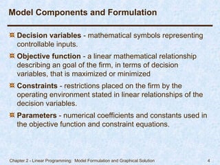
Decision variables - mathematical symbols representing
controllable inputs.
Objective function - a linear mathematical relationship
describing an goal of the firm, in terms of decision
variables, that is maximized or minimized
Constraints - restrictions placed on the firm by the
operating environment stated in linear relationships of the
decision variables.
Parameters - numerical coefficients and constants used in
the objective function and constraint equations.
Model Components and Formulation
5.
Chapter 2 -Linear Programming: Model Formulation and Graphical Solution 5
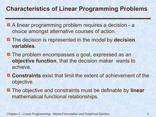
Characteristics of Linear Programming Problems
A linear programming problem requires a decision - a
choice amongst alternative courses of action.
The decision is represented in the model by decision
variables.
The problem encompasses a goal, expressed as an
objective function, that the decision maker wants to
achieve.
Constraints exist that limit the extent of achievement of the
objective.
The objective and constraints must be definable by linear
mathematical functional relationships.
6.
Chapter 2 -Linear Programming: Model Formulation and Graphical Solution 6
Objectiv
Objectiv
e
e
Function
Function
“
“Subject to”
Subject to”
Constraint
Constraint
s
s
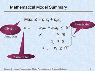
Mathematical Model Summary
Max: Z = p1x1 + p2x2
s.t. a1x1 + a2x2 < b
x1 > m
x2 < u
x1 , x2 > 0
7.
Chapter 2 -Linear Programming: Model Formulation and Graphical Solution 7
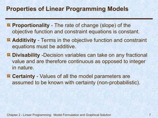
Proportionality - The rate of change (slope) of the
objective function and constraint equations is constant.
Additivity - Terms in the objective function and constraint
equations must be additive.
Divisability -Decision variables can take on any fractional
value and are therefore continuous as opposed to integer
in nature.
Certainty - Values of all the model parameters are
assumed to be known with certainty (non-probabilistic).
Properties of Linear Programming Models
8.
Chapter 2 -Linear Programming: Model Formulation and Graphical Solution 8
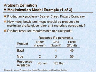
Resource Requirements
Product
Labor
(hr/unit)
Clay
(lb/unit)
Profit
($/unit)
Bowl 1 4 40
Mug 2 3 50
Resources
Available
40 hrs 120 lbs
Problem Definition
A Maximization Model Example (1 of 3)
Product mix problem - Beaver Creek Pottery Company
How many bowls and mugs should be produced to
maximize profits given labor and materials constraints?
Product resource requirements and unit profit:
9.
Chapter 2 -Linear Programming: Model Formulation and Graphical Solution 9
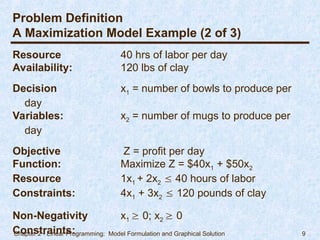
Problem Definition
A Maximization Model Example (2 of 3)
Resource 40 hrs of labor per day
Availability: 120 lbs of clay
Decision x1 = number of bowls to produce per
day
Variables: x2 = number of mugs to produce per
day
Objective Z = profit per day
Function: Maximize Z = $40x1 + $50x2
Resource 1x1 + 2x2 40 hours of labor
Constraints: 4x1 + 3x2 120 pounds of clay
Non-Negativity x1 0; x2 0
Constraints:
10.
Chapter 2 -Linear Programming: Model Formulation and Graphical Solution 10
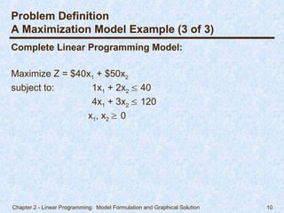
Problem Definition
A Maximization Model Example (3 of 3)
Complete Linear Programming Model:
Maximize Z = $40x1 + $50x2
subject to: 1x1 + 2x2 40
4x1 + 3x2 120
x1, x2 0
11.
Chapter 2 -Linear Programming: Model Formulation and Graphical Solution 11
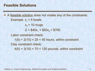
A feasible solution does not violate any of the constraints:
Example x1 = 5 bowls
x2 = 10 mugs
Z = $40x1 + $50x2 = $700
Labor constraint check:
1(5) + 2(10) = 25 < 40 hours, within constraint
Clay constraint check:
4(5) + 3(10) = 70 < 120 pounds, within constraint
Feasible Solutions
12.
Chapter 2 -Linear Programming: Model Formulation and Graphical Solution 12
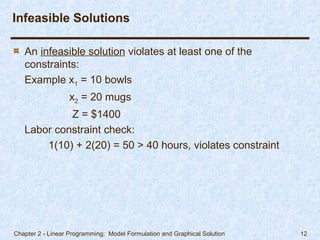
An infeasible solution violates at least one of the
constraints:
Example x1 = 10 bowls
x2 = 20 mugs
Z = $1400
Labor constraint check:
1(10) + 2(20) = 50 > 40 hours, violates constraint
Infeasible Solutions
13.
Chapter 2 -Linear Programming: Model Formulation and Graphical Solution 13
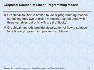
Graphical solution is limited to linear programming models
containing only two decision variables (can be used with
three variables but only with great difficulty).
Graphical methods provide visualization of how a solution
for a linear programming problem is obtained.
Graphical Solution of Linear Programming Models
14.
Chapter 2 -Linear Programming: Model Formulation and Graphical Solution 14
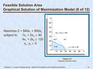
Feasible Solution Area
Graphical Solution of Maximization Model (6 of 12)
Maximize Z = $40x1 + $50x2
subject to: 1x1 + 2x2 40
4x1 + 3x2 120
x1, x2 0
Figure 2.6
Feasible Solution Area
15.
Chapter 2 -Linear Programming: Model Formulation and Graphical Solution 15
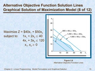
Alternative Objective Function Solution Lines
Graphical Solution of Maximization Model (8 of 12)
Maximize Z = $40x1 + $50x2
subject to: 1x1 + 2x2 40
4x1 + 3x2 120
x1, x2 0
Figure 2.8
Alternative Objective Function Lines
16.
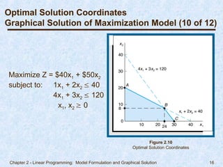
Chapter 2 -Linear Programming: Model Formulation and Graphical Solution 16
Optimal Solution Coordinates
Graphical Solution of Maximization Model (10 of 12)
Maximize Z = $40x1 + $50x2
subject to: 1x1 + 2x2 40
4x1 + 3x2 120
x1, x2 0
Figure 2.10
Optimal Solution Coordinates
17.
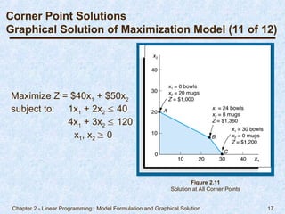
Chapter 2 -Linear Programming: Model Formulation and Graphical Solution 17
Corner Point Solutions
Graphical Solution of Maximization Model (11 of 12)
Maximize Z = $40x1 + $50x2
subject to: 1x1 + 2x2 40
4x1 + 3x2 120
x1, x2 0
Figure 2.11
Solution at All Corner Points
18.
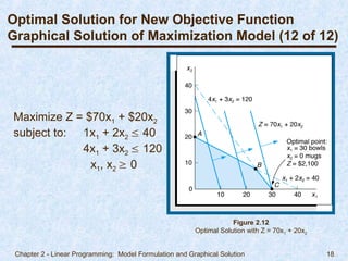
Chapter 2 -Linear Programming: Model Formulation and Graphical Solution 18
Optimal Solution for New Objective Function
Graphical Solution of Maximization Model (12 of 12)
Maximize Z = $70x1 + $20x2
subject to: 1x1 + 2x2 40
4x1 + 3x2 120
x1, x2 0
Figure 2.12
Optimal Solution with Z = 70x1 + 20x2
19.
Chapter 2 -Linear Programming: Model Formulation and Graphical Solution 19
Standard form requires that all constraints be in the form of
equations.
A slack variable is added to a constraint to convert it to
an equation (=).
A slack variable represents unused resources.
A slack variable contributes nothing to the objective function
value.
Slack Variables
20.
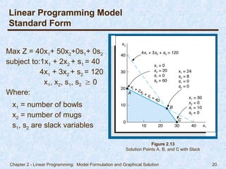
Chapter 2 -Linear Programming: Model Formulation and Graphical Solution 20
Linear Programming Model
Standard Form
Max Z = 40x1+ 50x2+0s1+ 0s2
subject to:1x1 + 2x2 + s1 = 40
4x1 + 3x2 + s2 = 120
x1, x2, s1, s2 0
Where:
x1 = number of bowls
x2 = number of mugs
s1, s2 are slack variables
Figure 2.13
Solution Points A, B, and C with Slack
21.
Chapter 2 -Linear Programming: Model Formulation and Graphical Solution 21
Problem Definition
A Minimization Model Example (1 of 7)
Chemical Contribution
Brand
Nitrogen
(lb/bag)
Phosphate
(lb/bag)
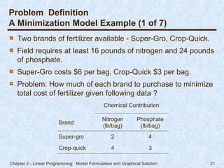
Super-gro 2 4
Crop-quick 4 3
Two brands of fertilizer available - Super-Gro, Crop-Quick.
Field requires at least 16 pounds of nitrogen and 24 pounds
of phosphate.
Super-Gro costs $6 per bag, Crop-Quick $3 per bag.
Problem: How much of each brand to purchase to minimize
total cost of fertilizer given following data ?
22.
Chapter 2 -Linear Programming: Model Formulation and Graphical Solution 22
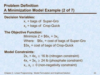
Problem Definition
A Minimization Model Example (2 of 7)
Decision Variables:
x1 = bags of Super-Gro
x2 = bags of Crop-Quick
The Objective Function:
Minimize Z = $6x1 + 3x2
Where: $6x1 = cost of bags of Super-Gro
$3x2 = cost of bags of Crop-Quick
Model Constraints:
2x1 + 4x2 16 lb (nitrogen constraint)
4x1 + 3x2 24 lb (phosphate constraint)
x1, x2 0 (non-negativity constraint)
23.
Chapter 2 -Linear Programming: Model Formulation and Graphical Solution 23
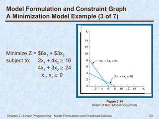
Model Formulation and Constraint Graph
A Minimization Model Example (3 of 7)
Minimize Z = $6x1 + $3x2
subject to: 2x1 + 4x2 16
4x1 + 3x2 24
x1, x2 0
Figure 2.14
Graph of Both Model Constraints
24.
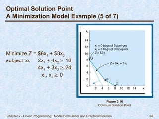
Chapter 2 -Linear Programming: Model Formulation and Graphical Solution 24
Optimal Solution Point
A Minimization Model Example (5 of 7)
Minimize Z = $6x1 + $3x2
subject to: 2x1 + 4x2 16
4x1 + 3x2 24
x1, x2 0
Figure 2.16
Optimum Solution Point
25.
Chapter 2 -Linear Programming: Model Formulation and Graphical Solution 25
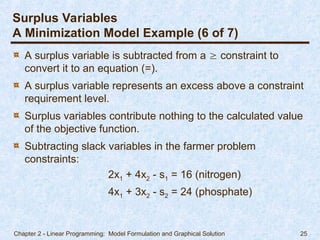
Surplus Variables
A Minimization Model Example (6 of 7)
A surplus variable is subtracted from a constraint to
convert it to an equation (=).
A surplus variable represents an excess above a constraint
requirement level.
Surplus variables contribute nothing to the calculated value
of the objective function.
Subtracting slack variables in the farmer problem
constraints:
2x1 + 4x2 - s1 = 16 (nitrogen)
4x1 + 3x2 - s2 = 24 (phosphate)
26.
Chapter 2 -Linear Programming: Model Formulation and Graphical Solution 26
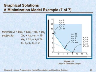
Minimize Z = $6x1 + $3x2 + 0s1 + 0s2
subject to: 2x1 + 4x2 – s1 = 16
4x2 + 3x2 – s2 = 24
x1, x2, s1, s2 0
Figure 2.17
Graph of Fertilizer Example
Graphical Solutions
A Minimization Model Example (7 of 7)
27.
Chapter 2 -Linear Programming: Model Formulation and Graphical Solution 27
For some linear programming models, the general rules do
not apply.
Special types of problems include those with:
Multiple optimal solutions
Infeasible solutions
Unbounded solutions
Special Cases of Linear Programming Problems
28.
Chapter 2 -Linear Programming: Model Formulation and Graphical Solution 28
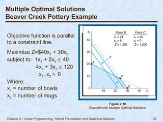
Objective function is parallel
to a constraint line.
Maximize Z=$40x1 + 30x2
subject to: 1x1 + 2x2 40
4x2 + 3x2 120
x1, x2 0
Where:
x1 = number of bowls
x2 = number of mugs
Figure 2.18
Example with Multiple Optimal Solutions
Multiple Optimal Solutions
Beaver Creek Pottery Example
29.
Chapter 2 -Linear Programming: Model Formulation and Graphical Solution 29
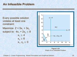
An Infeasible Problem
Every possible solution
violates at least one
constraint:
Maximize Z = 5x1 + 3x2
subject to: 4x1 + 2x2 8
x1 4
x2 6
x1, x2 0
Figure 2.19
Graph of an Infeasible Problem
30.
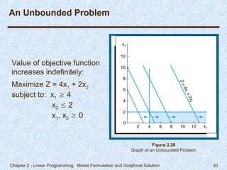
Chapter 2 -Linear Programming: Model Formulation and Graphical Solution 30
Value of objective function
increases indefinitely:
Maximize Z = 4x1 + 2x2
subject to: x1 4
x2 2
x1, x2 0
An Unbounded Problem
Figure 2.20
Graph of an Unbounded Problem
31.
Chapter 2 -Linear Programming: Model Formulation and Graphical Solution 31
Problem Statement
Example Problem No. 1 (1 of 3)
Hot dog mixture in 1000-pound batches.
Two ingredients, chicken ($3/lb) and beef ($5/lb).
Recipe requirements:
at least 500 pounds of chicken
at least 200 pounds of beef
Ratio of chicken to beef must be at least 2 to 1.
Determine optimal mixture of ingredients that will minimize
costs.
32.
Chapter 2 -Linear Programming: Model Formulation and Graphical Solution 32
Step 1:
Identify decision variables.
x1 = lb of chicken
x2 = lb of beef
Step 2:
Formulate the objective function.
Minimize Z = $3x1 + $5x2
where Z = cost per 1,000-lb batch
$3x1 = cost of chicken
$5x2 = cost of beef
Solution
Example Problem No. 1 (2 of 3)
33.
Chapter 2 -Linear Programming: Model Formulation and Graphical Solution 33
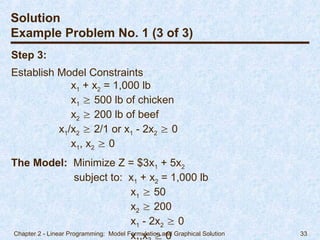
Solution
Example Problem No. 1 (3 of 3)
Step 3:
Establish Model Constraints
x1 + x2 = 1,000 lb
x1 500 lb of chicken
x2 200 lb of beef
x1/x2 2/1 or x1 - 2x2 0
x1, x2 0
The Model: Minimize Z = $3x1 + 5x2
subject to: x1 + x2 = 1,000 lb
x1 50
x2 200
x1 - 2x2 0
x ,x 0
34.
Chapter 2 -Linear Programming: Model Formulation and Graphical Solution 34
Solve the following model
graphically:
Maximize Z = 4x1 + 5x2
subject to: x1 + 2x2 10
6x1 + 6x2 36
x1 4
x1, x2 0
Step 1: Plot the constraints
as equations
Example Problem No. 2 (1 of 3)
Figure 2.21
Constraint Equations
35.
Chapter 2 -Linear Programming: Model Formulation and Graphical Solution 35
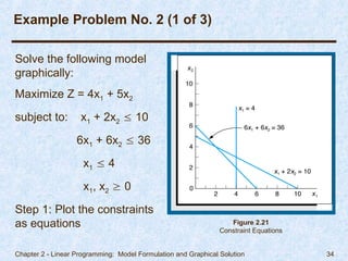
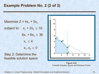
Example Problem No. 2 (2 of 3)
Maximize Z = 4x1 + 5x2
subject to: x1 + 2x2 10
6x1 + 6x2 36
x1 4
x1, x2 0
Step 2: Determine the
feasible solution space
Figure 2.22
Feasible Solution Space and Extreme Points
36.
Chapter 2 -Linear Programming: Model Formulation and Graphical Solution 36
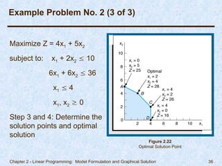
Example Problem No. 2 (3 of 3)
Maximize Z = 4x1 + 5x2
subject to: x1 + 2x2 10
6x1 + 6x2 36
x1 4
x1, x2 0
Step 3 and 4: Determine the
solution points and optimal
solution
Figure 2.22
Optimal Solution Point