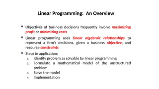
Objectives ofbusiness decisions frequently involve maximizing
profit or minimizing costs
Linear programming uses linear algebraic relationships to
represent a firm’s decisions, given a business objective, and
resource constraints
Steps in application:
1. Identify problem as solvable by linear programming
2. Formulate a mathematical model of the unstructured
problem
3. Solve the model
4. Implementation
Linear Programming: An Overview
4.
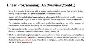
Linear Programming: AnOverview(Contd..)
• Linear Programming is the most widely applied mathematical technique that helps in decision
making and planning for the optimal allocation of limited resources.
• It deals with the optimization (maximization or minimization) of a function of variables known as
objective function, subject to a set of linear equations and/or inequalities known as constraints.
• The objective function may be profit, cost, production capacity or any other measure of
effectiveness, which is to be obtained in the best possible or optimal manner.
• The constraints may be imposed by different resources such as raw material availability, market
demand, production process and equipment, storage capacity etc.
• It helps in attaining the optimum use of productive factors. Linear programming indicates how a
manager can utilize his productive factors most effectively by a better selection and distribution of
these elements. For example, more efficient use of manpower and machines can be obtained by
the use of linear programming.
5.
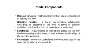
• Decision variables- mathematical symbols representing levels
of activity of a firm
• Objective function - a linear mathematical relationship
describing an objective of the firm, in terms of decision
variables - this function is to be maximized or minimized
• Constraints – requirements or restrictions placed on the firm
by the operating environment, stated in linear relationships of
the decision variables
• Parameters - numerical coefficients and constants used in the
objective function and constraints
Model Components
6.
Summary of ModelFormulation Steps
Step 1 : Clearly define the decision variables
Step 2 : Construct the objective function
Step 3 : Formulate the constraints
7.
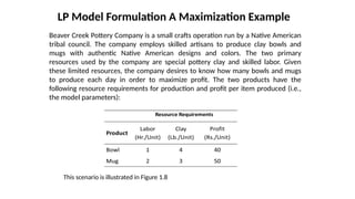
LP Model FormulationA Maximization Example
Beaver Creek Pottery Company is a small crafts operation run by a Native American
tribal council. The company employs skilled artisans to produce clay bowls and
mugs with authentic Native American designs and colors. The two primary
resources used by the company are special pottery clay and skilled labor. Given
these limited resources, the company desires to know how many bowls and mugs
to produce each day in order to maximize profit. The two products have the
following resource requirements for production and profit per item produced (i.e.,
the model parameters):
This scenario is illustrated in Figure 1.8
8.
LP Model Formulation
AMaximization Example (1 of 4)
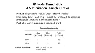
• Product mix problem - Beaver Creek Pottery Company
• How many bowls and mugs should be produced to maximize
profits given labor and materials constraints?
• Product resource requirements and unit profit:
Resource Requirements
Product
Labor
(Hr./Unit)
Clay
(Lb./Unit)
Profit
(Rs./Unit)
Bowl 1 4 40
Mug 2 3 50
Resource Availability: 40 hrs of labor per day
120 lbs of clay
9.
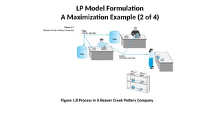
LP Model Formulation
AMaximization Example (2 of 4)
Figure 1.8 Process in A Beaver Creek Pottery Company
10.
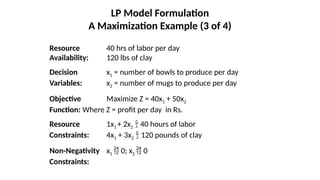
LP Model Formulation
AMaximization Example (3 of 4)
Resource 40 hrs of labor per day
Availability: 120 lbs of clay
Decision x1 = number of bowls to produce per day
Variables: x2 = number of mugs to produce per day
Objective Maximize Z = 40x1 + 50x2
Function: Where Z = profit per day in Rs.
Resource 1x1 + 2x2 40 hours of labor
Constraints: 4x1 + 3x2 120 pounds of clay
Non-Negativity x1 0; x2 0
Constraints:
11.
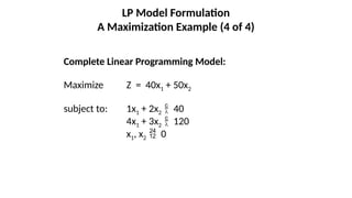
LP Model Formulation
AMaximization Example (4 of 4)
Complete Linear Programming Model:
Maximize Z = 40x1 + 50x2
subject to: 1x1 + 2x2 40
4x1 + 3x2 120
x1, x2 0
12.
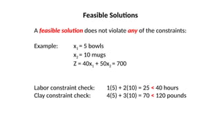
A feasible solutiondoes not violate any of the constraints:
Example: x1 = 5 bowls
x2 = 10 mugs
Z = 40x1 + 50x2 = 700
Labor constraint check: 1(5) + 2(10) = 25 < 40 hours
Clay constraint check: 4(5) + 3(10) = 70 < 120 pounds
Feasible Solutions
13.
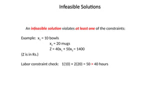
An infeasible solutionviolates at least one of the constraints:
Example: x1 = 10 bowls
x2 = 20 mugs
Z = 40x1 + 50x2 = 1400
(Z is in Rs.)
Labor constraint check: 1(10) + 2(20) = 50 > 40 hours
Infeasible Solutions
14.
• Graphical solutionis limited to linear programming
models containing only two decision variables (can
be used with three variables but only with great
difficulty)
• Graphical methods provide visualization of how a
solution for a linear programming problem is
obtained
Graphical Solution of LP Models
15.
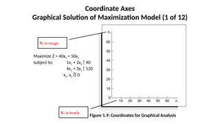
Coordinate Axes
Graphical Solutionof Maximization Model (1 of 12)
Figure 1.9: Coordinates for Graphical Analysis
Maximize Z = 40x1 + 50x2
subject to: 1x1 + 2x2 40
4x1 + 3x2 120
x1, x2 0
X1 is bowls
X2 is mugs
16.
Labor Constraint
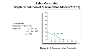
Graphical Solutionof Maximization Model (2 of 12)
Figure 1.10: Graph of Labor Constraint
Z is Profit in Rs.
Maximize Z = 40x1 + 50x2
subject to: 1x1 + 2x2 40
4x1 + 3x2 120
x1, x2 0
17.
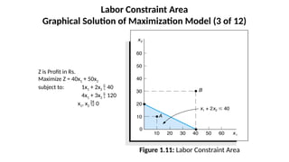
Labor Constraint Area
GraphicalSolution of Maximization Model (3 of 12)
Figure 1.11: Labor Constraint Area
Z is Profit in Rs.
Maximize Z = 40x1 + 50x2
subject to: 1x1 + 2x2 40
4x1 + 3x2 120
x1, x2 0
18.
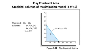
Clay Constraint Area
GraphicalSolution of Maximization Model (4 of 12)
Figure 1.12 : Clay Constraint Area
Maximize Z = 40x1 + 50x2
subject to: 1x1 + 2x2 40
4x1 + 3x2 120
x1, x2 0
19.
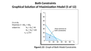
Both Constraints
Graphical Solutionof Maximization Model (5 of 12)
Figure1.13 : Graph of Both Model Constraints
Z is in Rs.
Maximize Z = 40x1 + 50x2
subject to: 1x1 + 2x2 40
4x1 + 3x2 120
x1, x2 0
20.
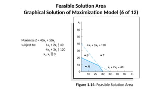
Feasible Solution Area
GraphicalSolution of Maximization Model (6 of 12)
Figure 1.14: Feasible Solution Area
Maximize Z = 40x1 + 50x2
subject to: 1x1 + 2x2 40
4x1 + 3x2 120
x1, x2 0
21.
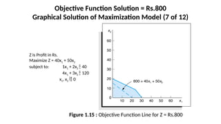
Objective Function Solution= Rs.800
Graphical Solution of Maximization Model (7 of 12)
Figure 1.15 : Objective Function Line for Z = Rs.800
Z is Profit in Rs.
Maximize Z = 40x1 + 50x2
subject to: 1x1 + 2x2 40
4x1 + 3x2 120
x1, x2 0
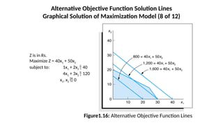
22.
Alternative Objective FunctionSolution Lines
Graphical Solution of Maximization Model (8 of 12)
Figure1.16: Alternative Objective Function Lines
Z is in Rs.
Maximize Z = 40x1 + 50x2
subject to: 1x1 + 2x2 40
4x1 + 3x2 120
x1, x2 0
23.
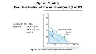
Optimal Solution
Graphical Solutionof Maximization Model (9 of 12)
Figure 1.17: Identification of Optimal Solution Point
Maximize Z = 40x1 + 50x2
subject to: 1x1 + 2x2 40
4x1 + 3x2 120
x1, x2 0
24.
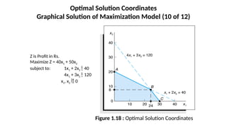
Optimal Solution Coordinates
GraphicalSolution of Maximization Model (10 of 12)
Figure 1.18 : Optimal Solution Coordinates
Z is Profit in Rs.
Maximize Z = 40x1 + 50x2
subject to: 1x1 + 2x2 40
4x1 + 3x2 120
x1, x2 0
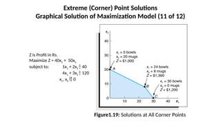
25.
Extreme (Corner) PointSolutions
Graphical Solution of Maximization Model (11 of 12)
Figure1.19: Solutions at All Corner Points
Z is Profit in Rs.
Maximize Z = 40x1 + 50x2
subject to: 1x1 + 2x2 40
4x1 + 3x2 120
x1, x2 0
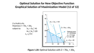
26.
Optimal Solution forNew Objective Function
Graphical Solution of Maximization Model (12 of 12)
Z is Profit in Rs.
Maximize Z = 70x1 + 20x2
subject to: 1x1 + 2x2 40
4x1+ 3x2 120
x1, x2 0
Figure 1.20: Optimal Solution with Z = 70x1 + 20x2
27.
Standard formrequires that all constraints be in the form of
equations (equalities)
A slack variable is added to a constraint (weak inequality) to
convert it to an equation (=)
A slack variable typically represents an unused resource
A slack variable contributes nothing to the objective function value
Slack Variables
28.
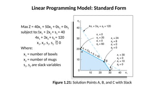
Linear Programming Model:Standard Form
Max Z = 40x1 + 50x2 + 0s1 + 0s2
subject to:1x1 + 2x2 + s1 = 40
4x1 + 3x2 + s2 = 120
x1, x2, s1, s2 0
Where:
x1 = number of bowls
x2 = number of mugs
s1, s2 are slack variables
Figure 1.21: Solution Points A, B, and C with Slack
29.
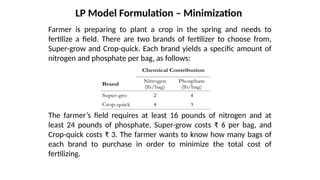
Farmer is preparingto plant a crop in the spring and needs to
fertilize a field. There are two brands of fertilizer to choose from,
Super-grow and Crop-quick. Each brand yields a specific amount of
nitrogen and phosphate per bag, as follows:
LP Model Formulation – Minimization
Chemical Contribution
Brand
Nitrogen
(lb/bag)
Phosphate
(lb/bag)
Super-gro 2 4
Crop-quick 4 3
The farmer’s field requires at least 16 pounds of nitrogen and at
least 24 pounds of phosphate. Super-grow costs ₹ 6 per bag, and
Crop-quick costs ₹ 3. The farmer wants to know how many bags of
each brand to purchase in order to minimize the total cost of
fertilizing.
30.
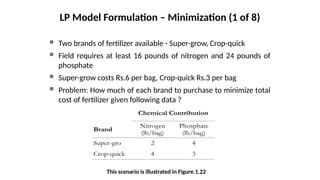
LP Model Formulation– Minimization (1 of 8)
Chemical Contribution
Brand
Nitrogen
(lb/bag)
Phosphate
(lb/bag)
Super-gro 2 4
Crop-quick 4 3
Two brands of fertilizer available - Super-grow, Crop-quick
Field requires at least 16 pounds of nitrogen and 24 pounds of
phosphate
Super-grow costs Rs.6 per bag, Crop-quick Rs.3 per bag
Problem: How much of each brand to purchase to minimize total
cost of fertilizer given following data ?
This scenario is illustrated in Figure.1.22
31.
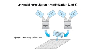
LP Model Formulation– Minimization (2 of 8)
Figure1.22: Fertilizing farmer’s field
32.
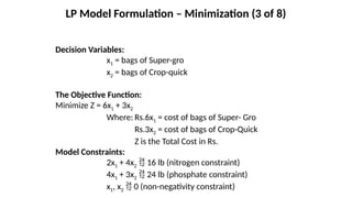
Decision Variables:
x1 =bags of Super-gro
x2 = bags of Crop-quick
The Objective Function:
Minimize Z = 6x1 + 3x2
Where: Rs.6x1 = cost of bags of Super- Gro
Rs.3x2 = cost of bags of Crop-Quick
Z is the Total Cost in Rs.
Model Constraints:
2x1 + 4x2 16 lb (nitrogen constraint)
4x1 + 3x2 24 lb (phosphate constraint)
x1, x2 0 (non-negativity constraint)
LP Model Formulation – Minimization (3 of 8)
33.
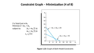
Z is TotalCost in Rs.
Minimize Z = 6x1 + 3x2
subject to: 2x1 + 4x2 16
4x1 + 3x2 24
x1, x2 0
Figure 1.23: Graph of Both Model Constraints
Constraint Graph – Minimization (4 of 8)
34.
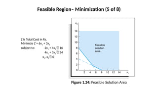
Figure 1.24: FeasibleSolution Area
Feasible Region– Minimization (5 of 8)
Z is Total Cost in Rs.
Minimize Z = 6x1 + 3x2
subject to: 2x1 + 4x2 16
4x1 + 3x2 24
x1, x2 0
35.
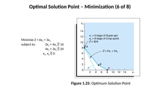
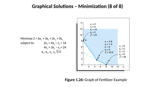
Figure 1.25: OptimumSolution Point
Optimal Solution Point – Minimization (6 of 8)
Minimize Z = 6x1 + 3x2
subject to: 2x1 + 4x2 16
4x1 + 3x2 24
x1, x2 0
36.
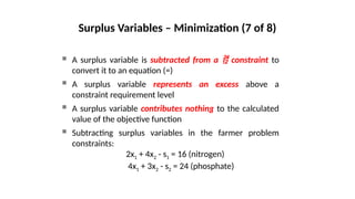
A surplusvariable is subtracted from a constraint to
convert it to an equation (=)
A surplus variable represents an excess above a
constraint requirement level
A surplus variable contributes nothing to the calculated
value of the objective function
Subtracting surplus variables in the farmer problem
constraints:
2x1 + 4x2 - s1 = 16 (nitrogen)
4x1 + 3x2 - s2 = 24 (phosphate)
Surplus Variables – Minimization (7 of 8)
For some linearprogramming models, the general rules do
not apply.
• Special types of problems include those with:
Multiple optimal solutions
Infeasible solutions
Unbounded solutions
Irregular Types of Linear Programming Problems
39.
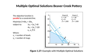
Figure 1.27: Examplewith Multiple Optimal Solutions
Multiple Optimal Solutions Beaver Creek Pottery
The objective function is
parallel to a constraint line.
Maximize Z=40x1 + 30x2
subject to: 1x1 + 2x2 40
4x1 + 3x2 120
x1, x2 0
Where:
x1 = number of bowls
x2 = number of mugs
40.
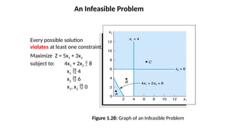
An Infeasible Problem
Figure1.28: Graph of an Infeasible Problem
Every possible solution
violates at least one constraint:
Maximize Z = 5x1 + 3x2
subject to: 4x1 + 2x2 8
x1 4
x2 6
x1, x2 0
41.
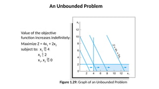
An Unbounded Problem
Figure1.29: Graph of an Unbounded Problem
Value of the objective
function increases indefinitely:
Maximize Z = 4x1 + 2x2
subject to: x1 4
x2 2
x1, x2 0
42.
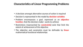
Characteristics of LinearProgramming Problems
• A decision amongst alternative courses of action is required
• Decision is represented in the model by decision variables
• Problem encompasses a goal, expressed as an objective
function, that the decision maker wants to achieve
• Restrictions (represented by constraints) exist that limit the
extent of achievement of the objective
• The objective and constraints must be definable by linear
mathematical functional relationships
43.
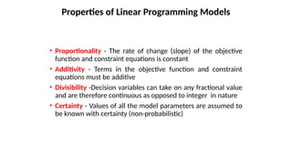
• Proportionality -The rate of change (slope) of the objective
function and constraint equations is constant
• Additivity - Terms in the objective function and constraint
equations must be additive
• Divisibility -Decision variables can take on any fractional value
and are therefore continuous as opposed to integer in nature
• Certainty - Values of all the model parameters are assumed to
be known with certainty (non-probabilistic)
Properties of Linear Programming Models
44.
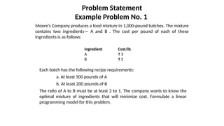
Moore’s Company producesa food mixture in 1,000-pound batches. The mixture
contains two ingredients— A and B . The cost per pound of each of these
ingredients is as follows:
Problem Statement
Example Problem No. 1
Each batch has the following recipe requirements:
a. At least 500 pounds of A
b. At least 200 pounds of B
The ratio of A to B must be at least 2 to 1. The company wants to know the
optimal mixture of ingredients that will minimize cost. Formulate a linear
programming model for this problem.
Ingredient Cost/lb.
A ₹ 3
B ₹ 5
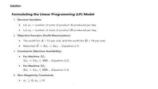
45.
Problem Statement
Example ProblemNo. 1 (1 of 3)
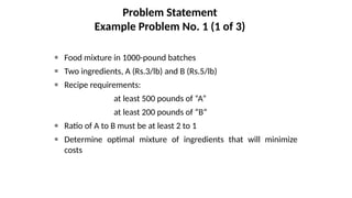
■ Food mixture in 1000-pound batches
■ Two ingredients, A (Rs.3/lb) and B (Rs.5/lb)
■ Recipe requirements:
at least 500 pounds of “A”
at least 200 pounds of “B”
■ Ratio of A to B must be at least 2 to 1
■ Determine optimal mixture of ingredients that will minimize
costs
46.
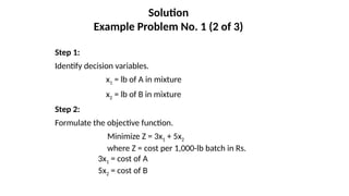
Step 1:
Identify decisionvariables.
x1 = lb of A in mixture
x2 = lb of B in mixture
Step 2:
Formulate the objective function.
Minimize Z = 3x1 + 5x2
where Z = cost per 1,000-lb batch in Rs.
3x1 = cost of A
5x2 = cost of B
Solution
Example Problem No. 1 (2 of 3)
47.
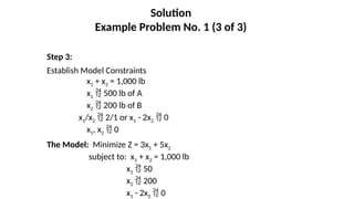
Step 3:
Establish ModelConstraints
x1 + x2 = 1,000 lb
x1 500 lb of A
x2 200 lb of B
x1/x2 2/1 or x1 - 2x2 0
x1, x2 0
The Model: Minimize Z = 3x1 + 5x2
subject to: x1 + x2 = 1,000 lb
x1 50
x2 200
x1 - 2x2 0
Solution
Example Problem No. 1 (3 of 3)
48.
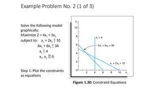
Solve the followingmodel
graphically:
Maximize Z = 4x1 + 5x2
subject to: x1 + 2x2 10
6x1 + 6x2 36
x1 4
x1, x2 0
Step 1: Plot the constraints
as equations
Example Problem No. 2 (1 of 3)
Figure 1.30: Constraint Equations
49.
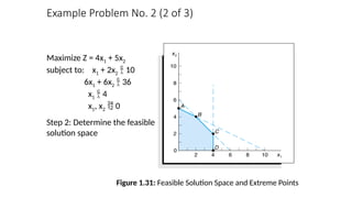
Example Problem No.2 (2 of 3)
Maximize Z = 4x1 + 5x2
subject to: x1 + 2x2 10
6x1 + 6x2 36
x1 4
x1, x2 0
Step 2: Determine the feasible
solution space
Figure 1.31: Feasible Solution Space and Extreme Points
50.
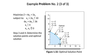
Example Problem No.2 (3 of 3)
Maximize Z = 4x1 + 5x2
subject to: x1 + 2x2 10
6x1 + 6x2 36
x1 4
x1, x2 0
Step 3 and 4: Determine the
solution points and optimal
solution
Figure 1.32: Optimal Solution Point
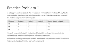
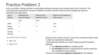
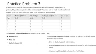
Practice Problem 2
Afirm uses lathes, milling machines, and grinding machines to produce two machine parts, Part I and Part II. The
machining times required for each part on different machines and the maximum time available per week are
provided in the table below:
Determine the number of parts I and II to be manufactured per week
in order to maximize the total profit.
1.Formulate the problem as a Linear Programming (LP) model by
defining:
1. The objective function to maximize profit
2. All constraints based on machining times and the maximum
time available for each machine
2.Ensure to include non-negativity constraints for the solution.
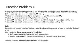
Practice Problem 4
Acompany manufactures two products, A and B, with profits earned per unit of ₹3 and ₹4, respectively.
Each product is processed on two machines, M₁ and M₂.
•Product A requires one minute of processing time on M₁ and two minutes on M₂.
•Product B requires one minute on M₁ and one minute on M₂.
•Machine M₁ is available for a maximum of 7 hours and 30 minutes (450 minutes) per working day.
•Machine M₂ is available for a maximum of 10 hours (600 minutes) per working day.
Task:
Determine the number of units of products A and B to be produced per day in order to maximize the total
profit.
1.Formulate the Linear Programming (LP) model by:
1. Defining the objective function for profit maximization.
2. Writing the constraints based on the availability of machine time on M₁ and M₂.
2.Ensure to include non-negativity constraints for the solution.
Summary
• Introduction tothe concepts of Management Science/Operations
Research has been discussed with reference to origin, history,
application
• Several illustrations have been used to formulate the Linear
Programming Problem in relation to objective function and
constraints
• The meaning of Feasible and Infeasible solutions has been discussed
graphically
• Demonstration of Maximisation and Minimisation problems has
been done graphically
• Examples of Bounded and Unbounded solutions have been
graphically analysed
57.
References
• Heaussler EF , Paul RW (2017), Introductory Mathematical Analysis, Pearson
Education
• Trivedi K and Trivedi C (2011) Business Mathematics, Pearson Education
• Dowling, Edward (2011), Schaum's Outline of Introduction to Mathematical
Economics, 3rd edition, McGraw-Hill Education
58.
Disclaimer
• All dataand content provided in this presentation are
taken from the reference books, internet – websites
and links, for informational purposes only.


![Ms(lpgraphicalsoln.)[1]](https://cdn.slidesharecdn.com/ss_thumbnails/mslpgraphicalsoln-150322191407-conversion-gate01-thumbnail.jpg?width=640&height=640&fit=bounds)


