Analysis

1. EXPLORING THE
REGRESSION ANALYSIS
CHAPTER 6 l LESSON 3 l STATISTICS AND PROBABILITY

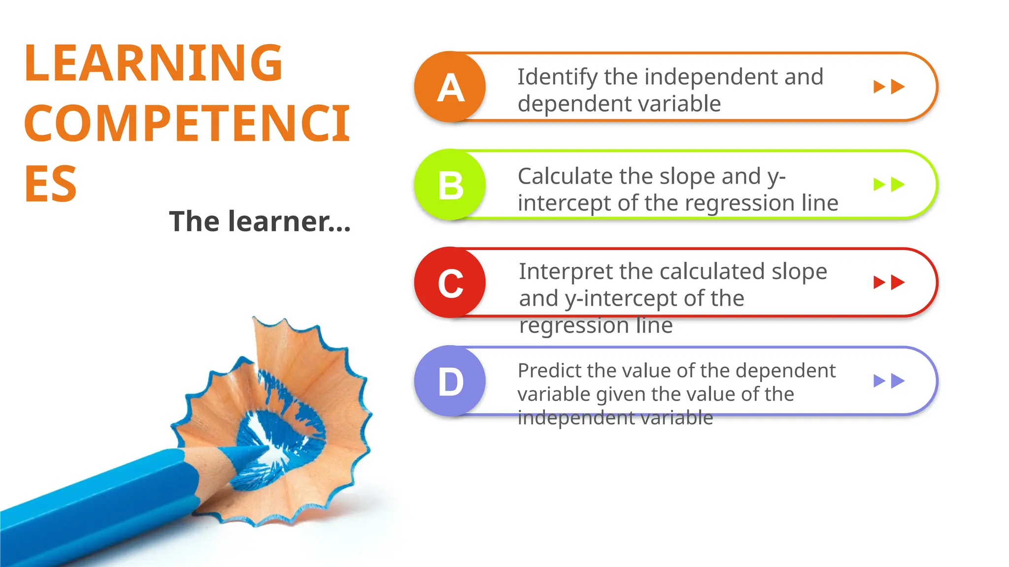
2. Identify the independent and
dependent variable
A
B
C
D
LEARNING
COMPETENCI
ES
The learner…
Calculate the slope and y-
intercept of the regression line
Interpret the calculated slope
and y-intercept of the
regression line
Predict the value of the dependent
variable given the value of the
independent variable

3. TESTING THE SIGNIFICANCE
OF r

4. The formula for the test statistic,
where df = n – 2

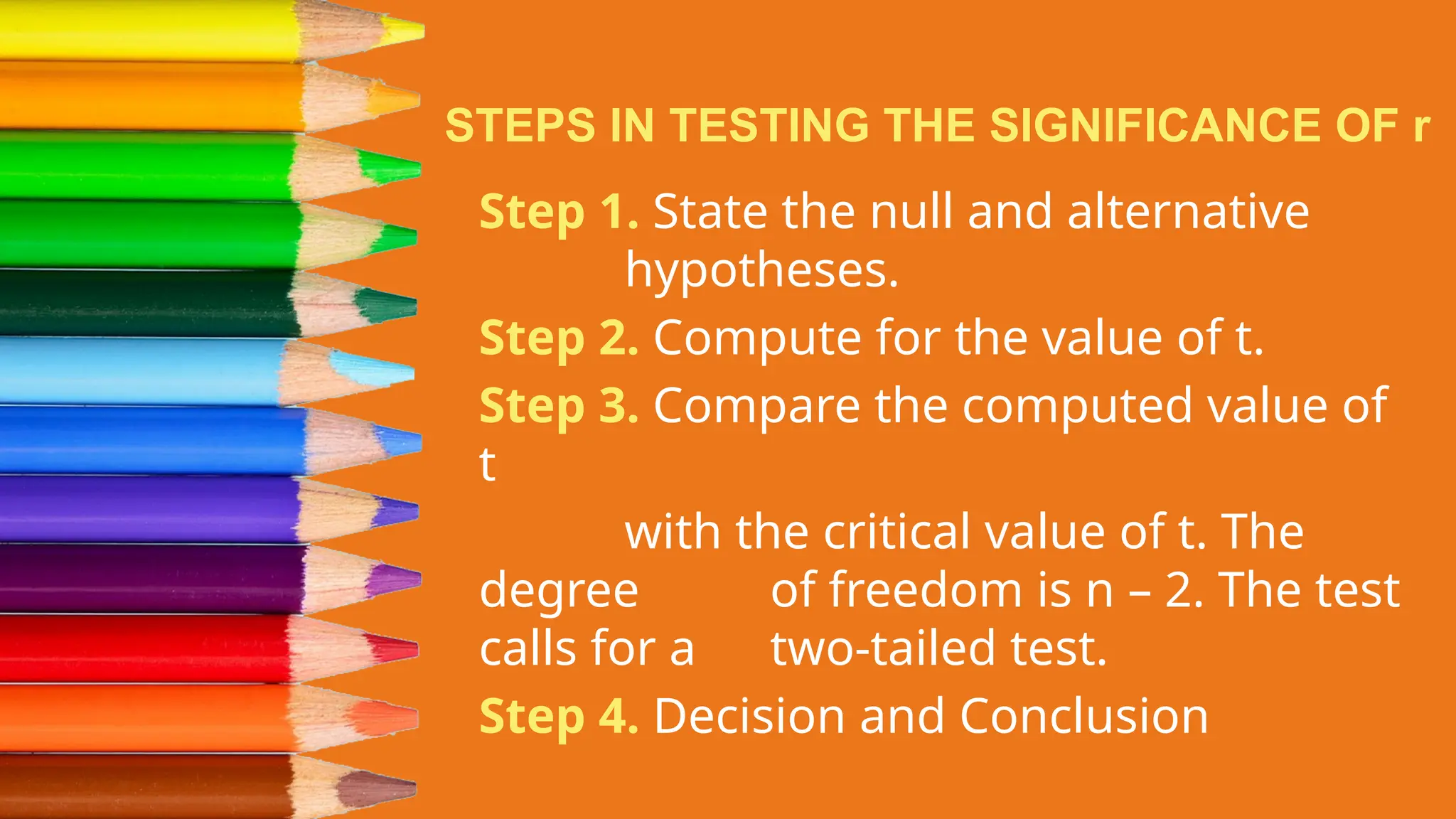
5. STEPS IN TESTING THE SIGNIFICANCE OF r
Step 1. State the null and alternative
hypotheses.
Step 2. Compute for the value of t.
Step 3. Compare the computed value of
t
with the critical value of t. The
degree of freedom is n – 2. The test
calls for a two-tailed test.
Step 4. Decision and Conclusion

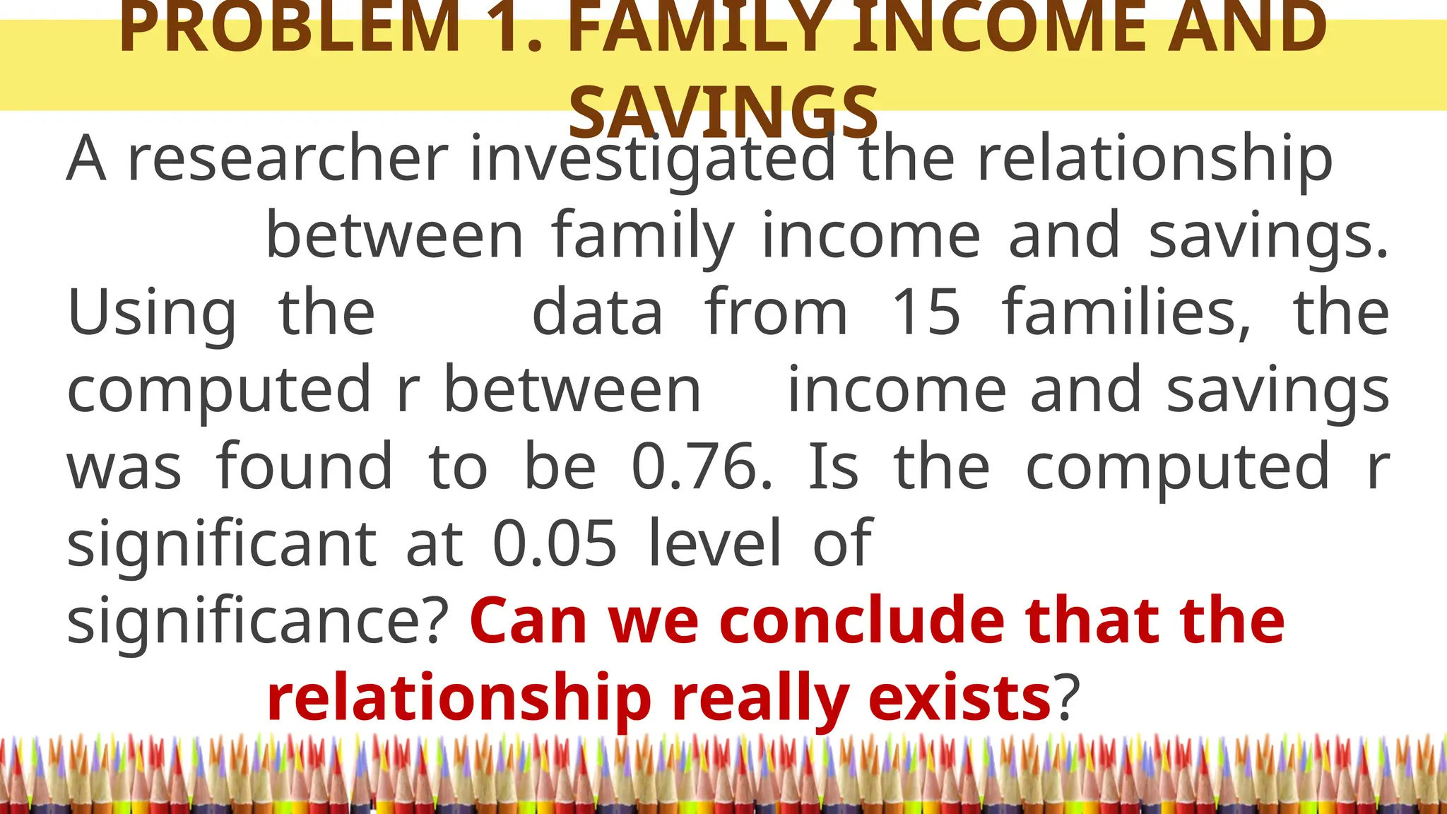
6. PROBLEM 1. FAMILY INCOME AND
SAVINGS
A researcher investigated the relationship
between family income and savings.
Using the data from 15 families, the
computed r between income and savings
was found to be 0.76. Is the computed r
significant at 0.05 level of
significance? Can we conclude that the
relationship really exists?

7. PROBLEM 1. FAMILY INCOME AND
SAVINGS
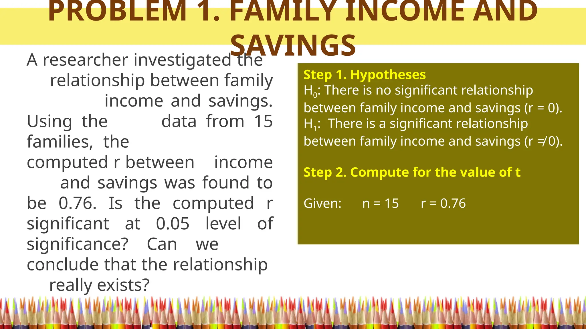
A researcher investigated the
relationship between family
income and savings.
Using the data from 15
families, the
computed r between income
and savings was found to
be 0.76. Is the computed r
significant at 0.05 level of
significance? Can we
conclude that the relationship
really exists?
Step 1. Hypotheses
H0: There is no significant relationship
between family income and savings (r = 0).
H1: There is a significant relationship
between family income and savings (r ≠ 0).
Step 2. Compute for the value of t
Given: n = 15 r = 0.76

8. PROBLEM 1. FAMILY INCOME AND
SAVINGS
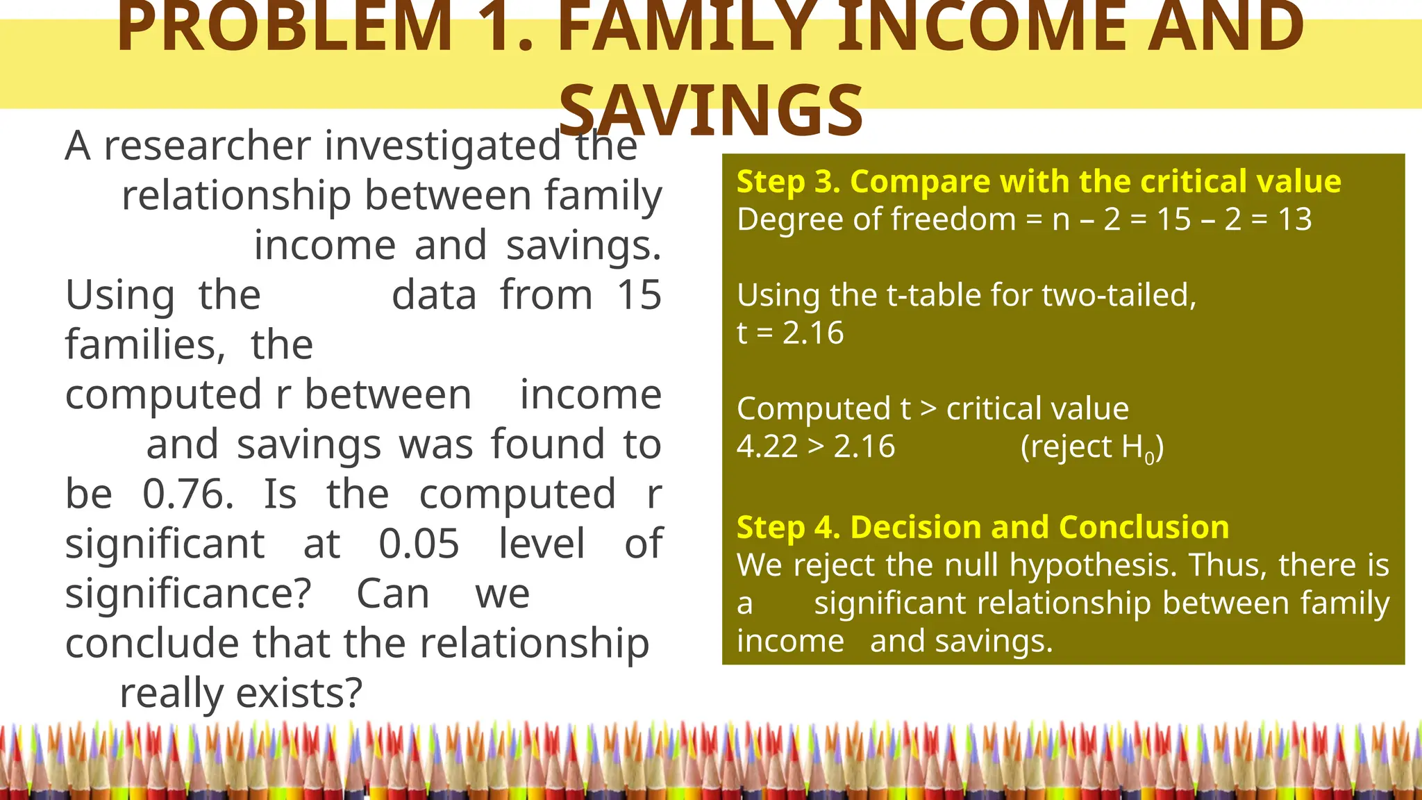
A researcher investigated the
relationship between family
income and savings.
Using the data from 15
families, the
computed r between income
and savings was found to
be 0.76. Is the computed r
significant at 0.05 level of
significance? Can we
conclude that the relationship
really exists?
Step 3. Compare with the critical value
Degree of freedom = n – 2 = 15 – 2 = 13
Using the t-table for two-tailed,
t = 2.16
Computed t > critical value
4.22 > 2.16 (reject H0)
Step 4. Decision and Conclusion
We reject the null hypothesis. Thus, there is
a significant relationship between family
income and savings.

9. PROBLEM 2. IQ SCORES AND AGE
A researcher would like to know if IQ scores
are related to age. Using 10 high school
students, he found out that computed r is
0.58. At 0.05 level of significance, can he
conclude that the relationship
really exists in the population?

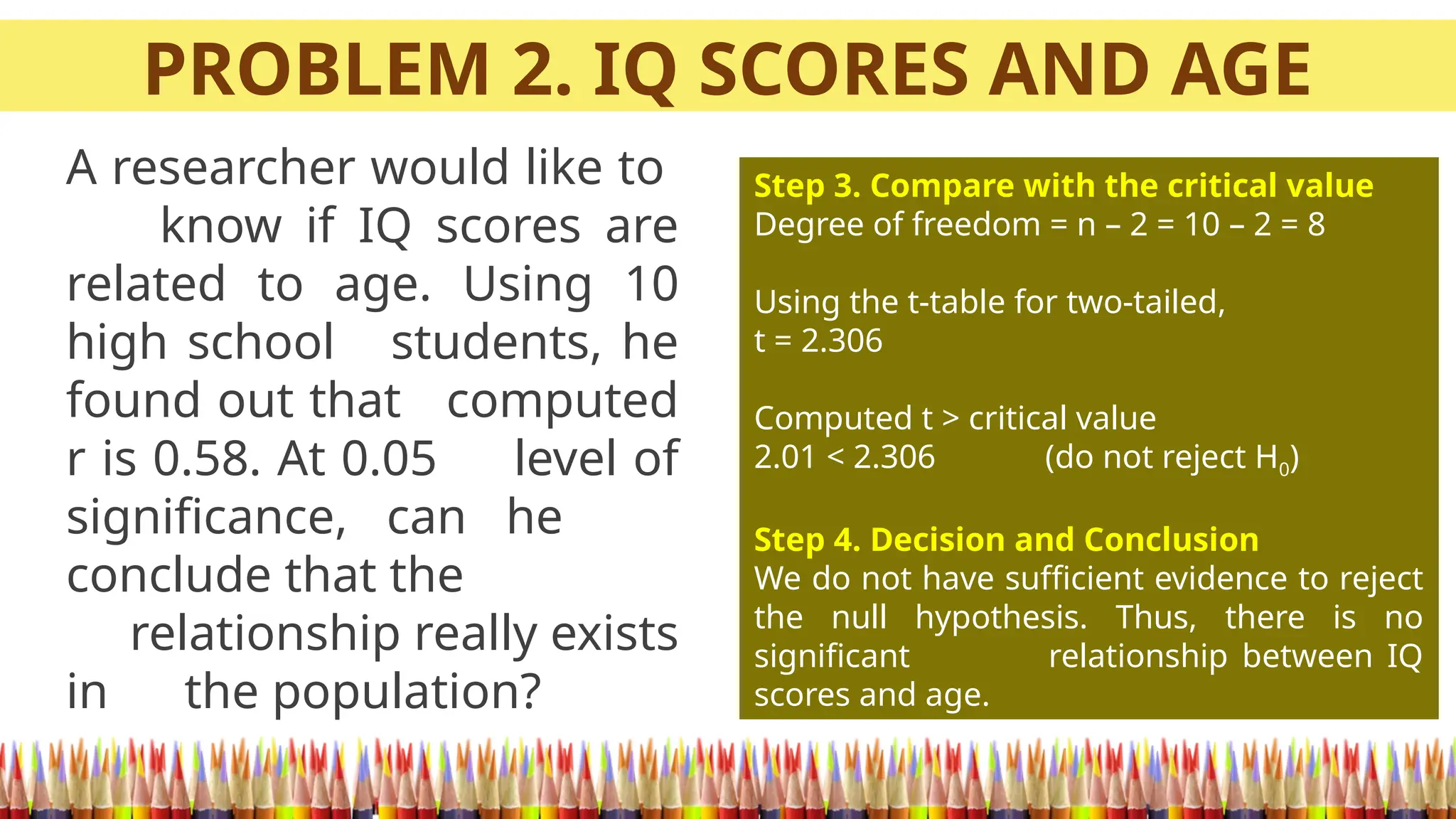
10. PROBLEM 2. IQ SCORES AND AGE
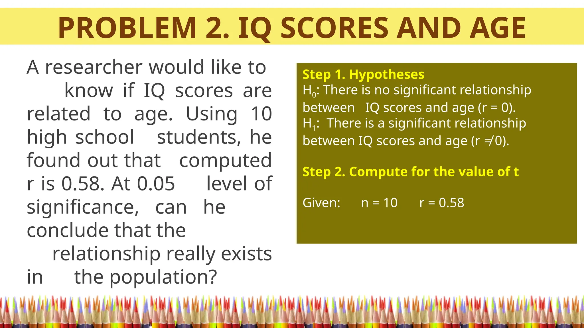
A researcher would like to
know if IQ scores are
related to age. Using 10
high school students, he
found out that computed
r is 0.58. At 0.05 level of
significance, can he
conclude that the
relationship really exists
in the population?
Step 1. Hypotheses
H0: There is no significant relationship
between IQ scores and age (r = 0).
H1: There is a significant relationship
between IQ scores and age (r ≠ 0).
Step 2. Compute for the value of t
Given: n = 10 r = 0.58

11. PROBLEM 2. IQ SCORES AND AGE
A researcher would like to
know if IQ scores are
related to age. Using 10
high school students, he
found out that computed
r is 0.58. At 0.05 level of
significance, can he
conclude that the
relationship really exists
in the population?
Step 3. Compare with the critical value
Degree of freedom = n – 2 = 10 – 2 = 8
Using the t-table for two-tailed,
t = 2.306
Computed t > critical value
2.01 < 2.306 (do not reject H0)
Step 4. Decision and Conclusion
We do not have sufficient evidence to reject
the null hypothesis. Thus, there is no
significant relationship between IQ
scores and age.

12. Note: If the computed r is
significant, the regression analysis
can be performed.

13. DEPENDENT AND
INDEPENDENT VARIABLES

14. Dependent variables
Are variables that are being predicted
or explained

15. Independent variables
Are variables that are being used to
predict or explain the dependent variables

16. When two variables are related,
one is the dependent variable while
the other is the independent
variable.

17. “ depends upon .”

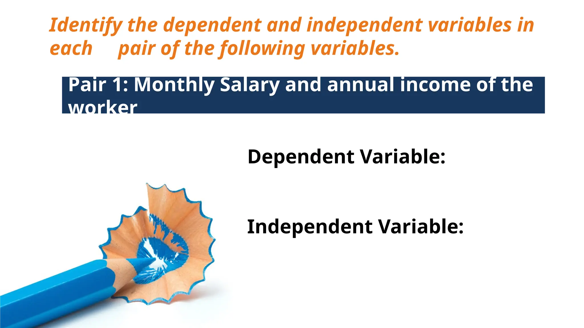
18. Identify the dependent and independent variables in
each pair of the following variables.
Pair 1: Monthly Salary and annual income of the
worker
Dependent Variable:
Independent Variable:

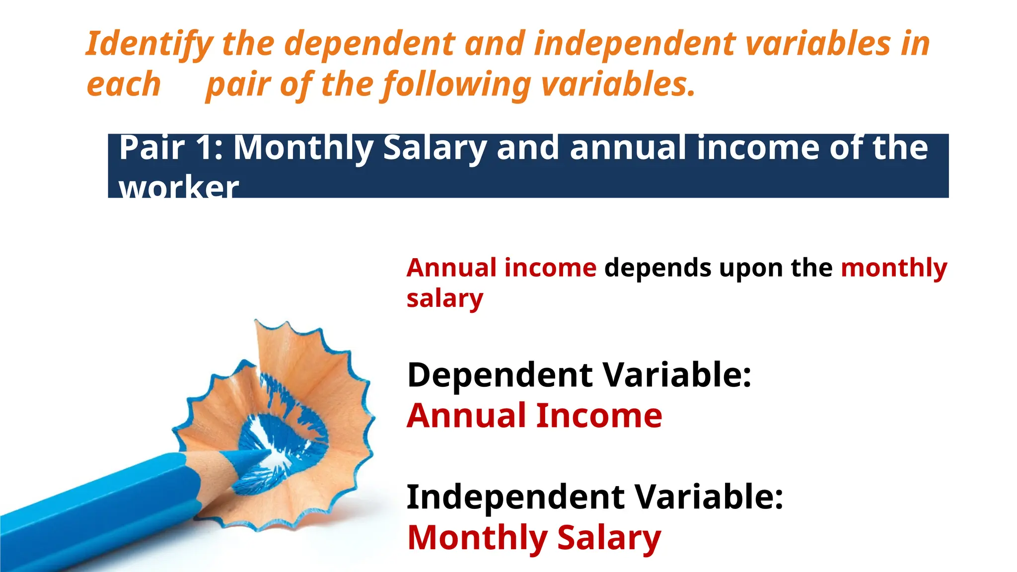
19. Identify the dependent and independent variables in
each pair of the following variables.
Pair 1: Monthly Salary and annual income of the
worker
Annual income depends upon the monthly
salary
Dependent Variable:
Annual Income
Independent Variable:
Monthly Salary

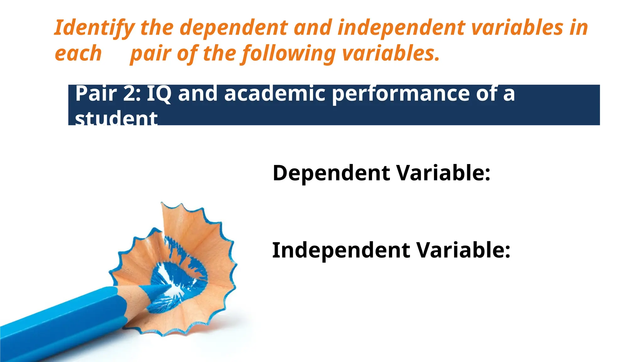
20. Identify the dependent and independent variables in
each pair of the following variables.
Pair 2: IQ and academic performance of a
student
Dependent Variable:
Independent Variable:

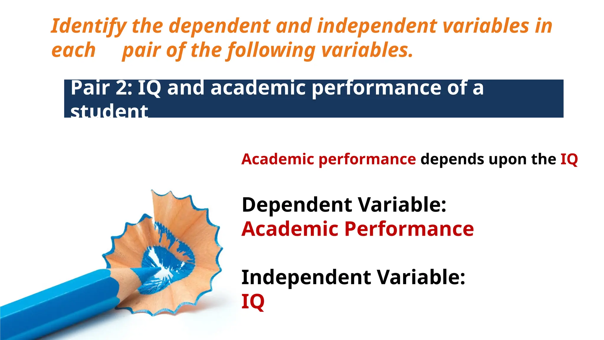
21. Identify the dependent and independent variables in
each pair of the following variables.
Pair 2: IQ and academic performance of a
student
Academic performance depends upon the IQ
Dependent Variable:
Academic Performance
Independent Variable:
IQ

22. Identify the dependent and independent variables in
each pair of the following variables.
Pair 3: Temperature and volume of air in a
balloon
Dependent Variable:
Independent Variable:

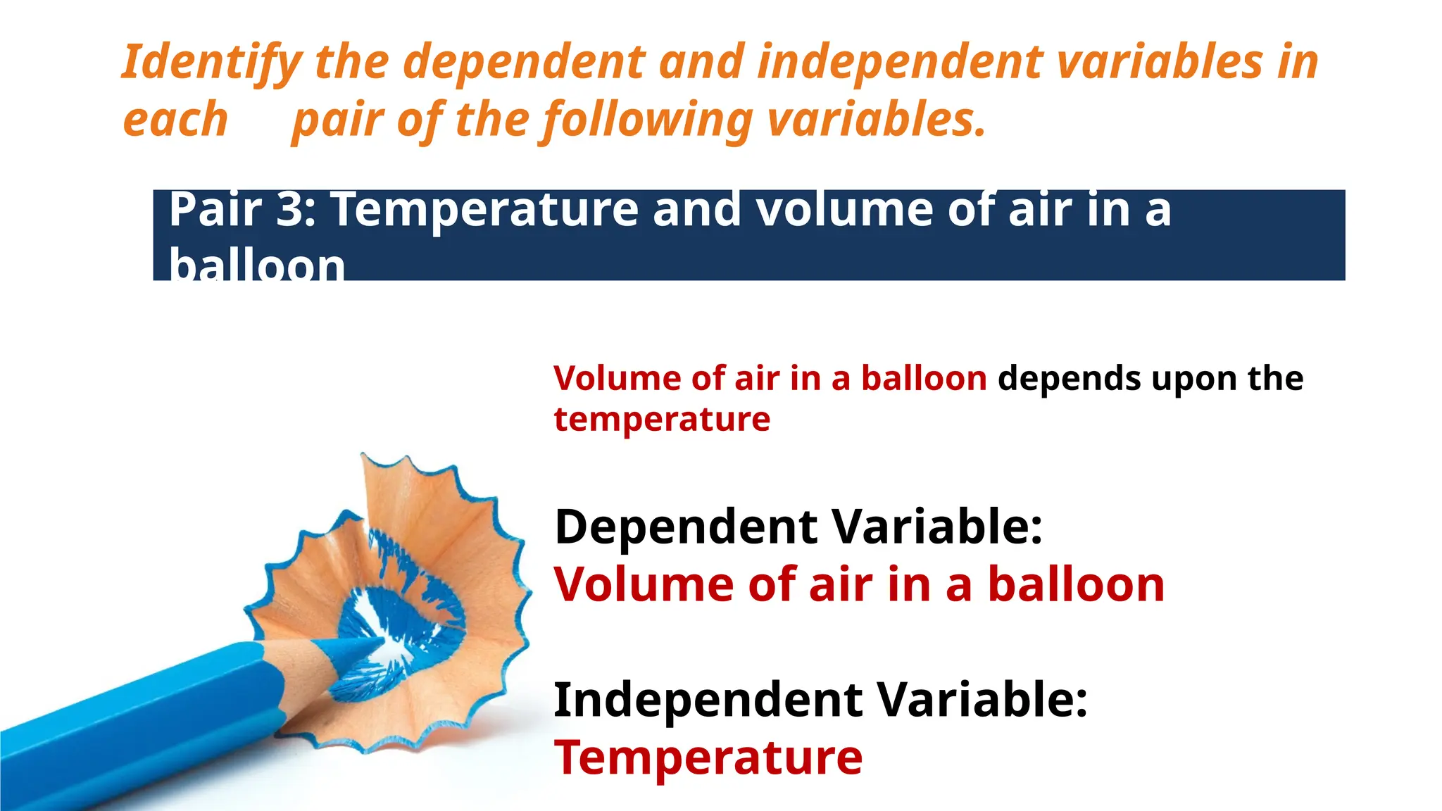
23. Identify the dependent and independent variables in
each pair of the following variables.
Pair 3: Temperature and volume of air in a
balloon
Volume of air in a balloon depends upon the
temperature
Dependent Variable:
Volume of air in a balloon
Independent Variable:
Temperature

24. Identify the dependent and independent variables in
each pair of the following variables.
Pair 4: Altitude and acceleration due to gravity
Dependent Variable:
Independent Variable:

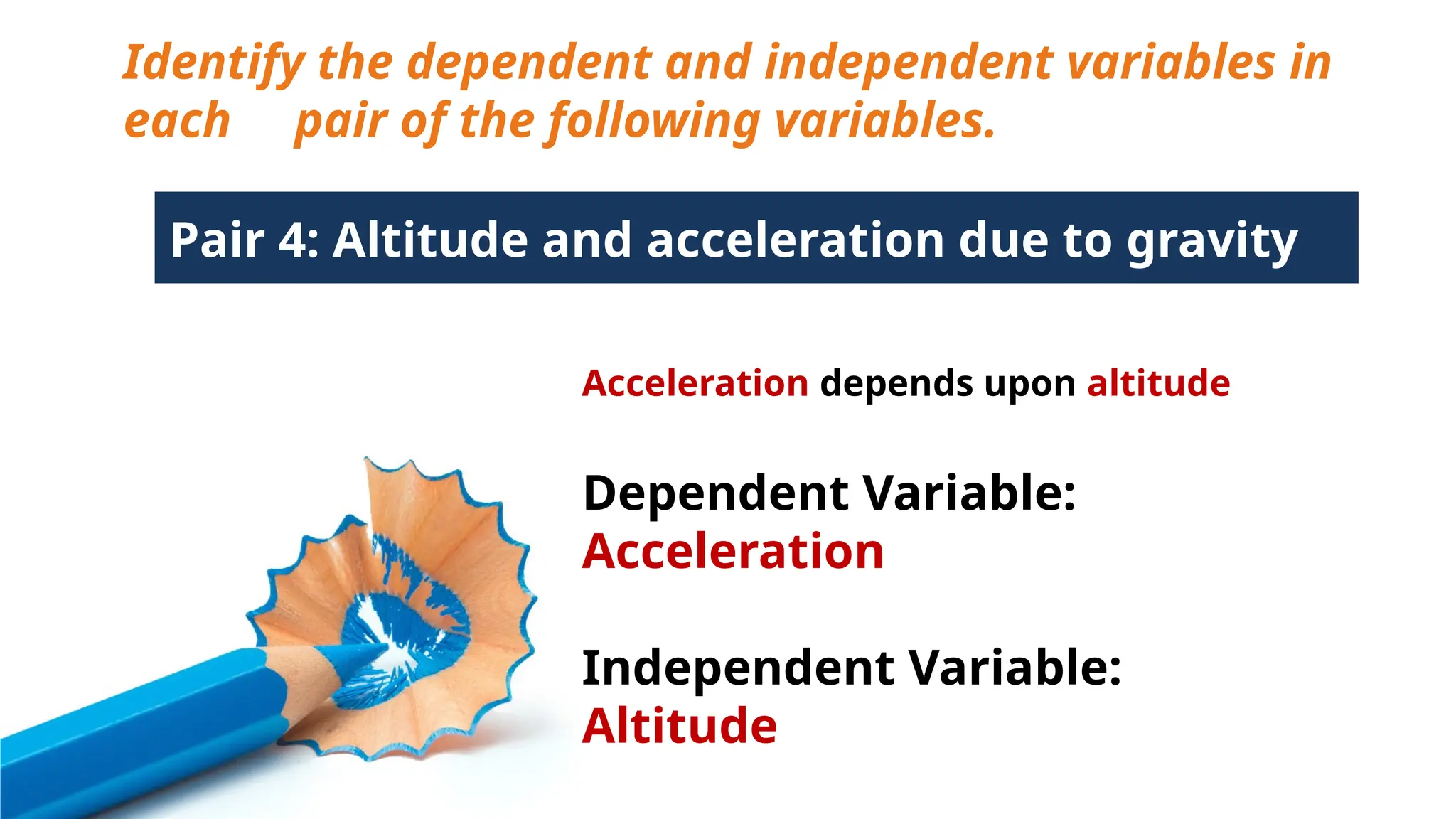
25. Identify the dependent and independent variables in
each pair of the following variables.
Pair 4: Altitude and acceleration due to gravity
Acceleration depends upon altitude
Dependent Variable:
Acceleration
Independent Variable:
Altitude

26. Identify the dependent and independent variables in
each pair of the following variables.
Pair 5: Demand and price of goods
Dependent Variable:
Independent Variable:

27. Identify the dependent and independent variables in
each pair of the following variables.
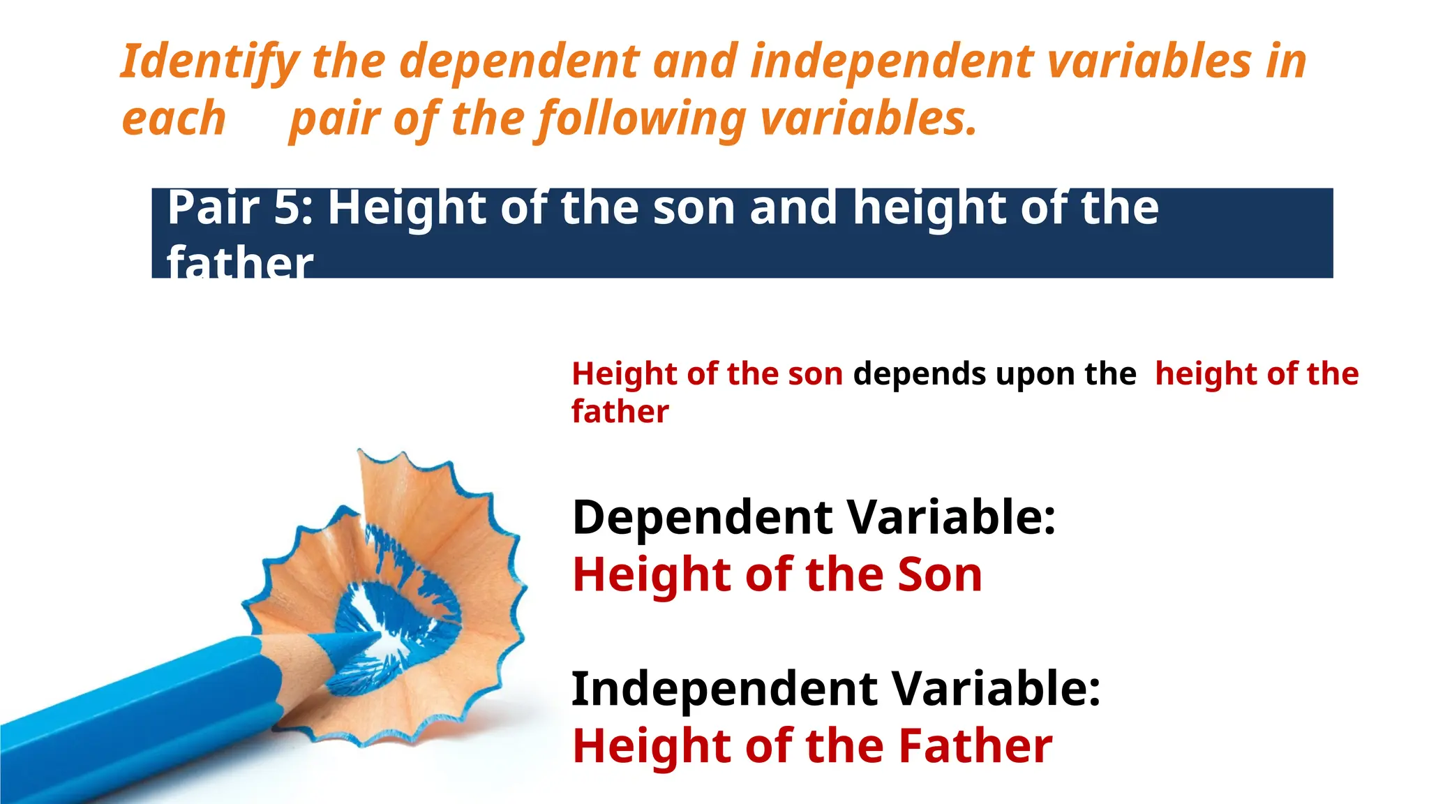
Pair 5: Height of the son and height of the
father
Height of the son depends upon the height of the
father
Dependent Variable:
Height of the Son
Independent Variable:
Height of the Father

28. TREND LINE
The line “closest” to the points in the
scatterplot

31. The points in the
scatterplot regress with
reference to

32. The regression line is the
same as the trend line.

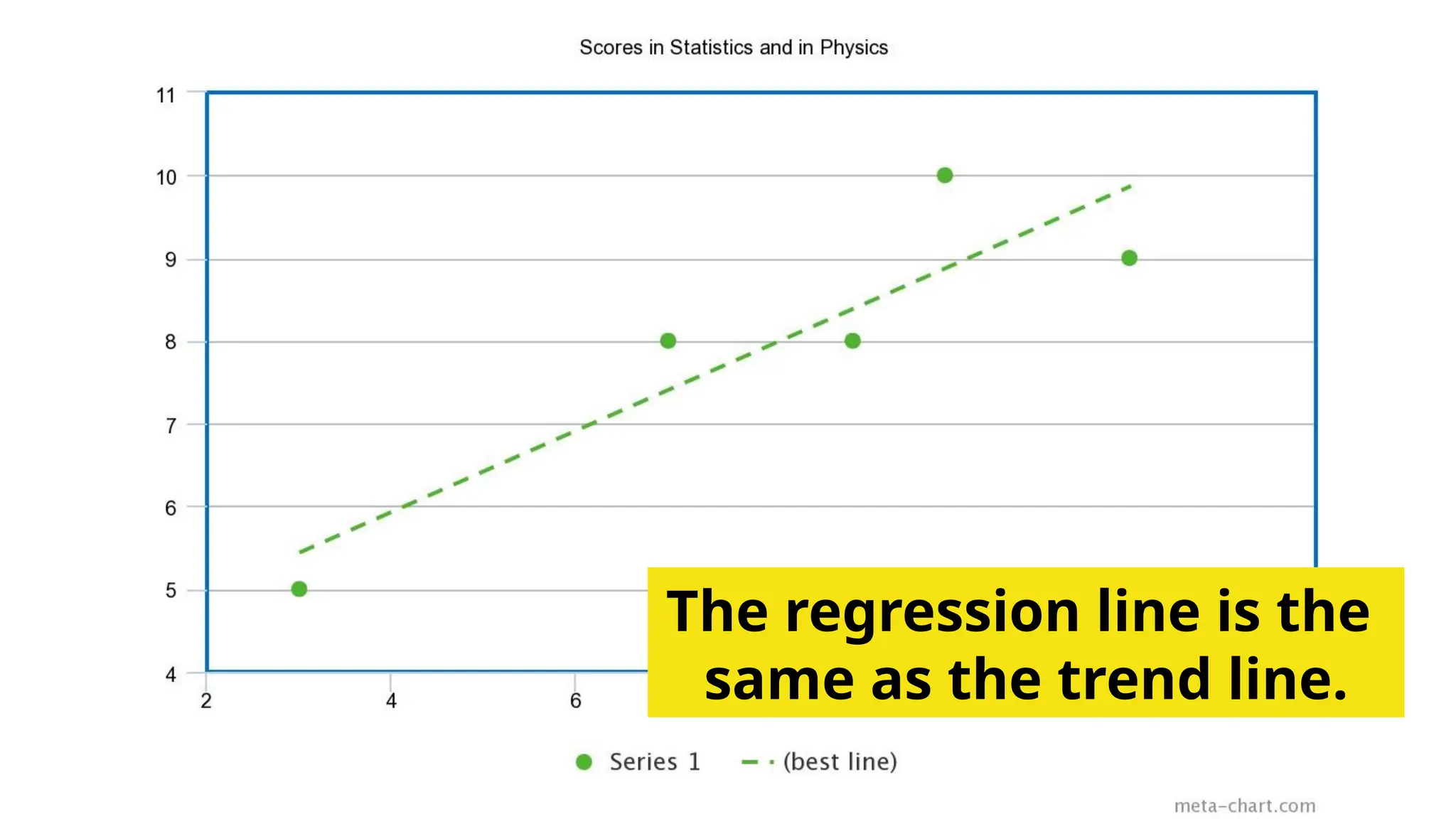
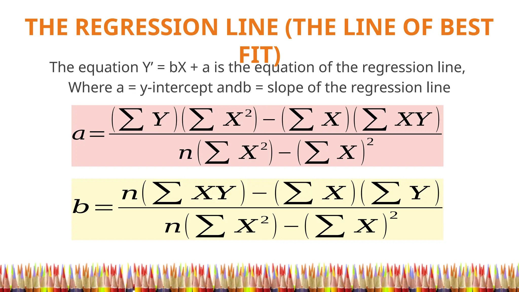
33. THE REGRESSION LINE (THE LINE OF BEST
FIT)
The equation Y’ = bX + a is the equation of the regression line,
Where a = y-intercept andb = slope of the regression line
𝑎=
(∑ 𝑌 )(∑ 𝑋2
)− (∑ 𝑋 )(∑ 𝑋𝑌 )
𝑛 (∑ 𝑋
2
)− (∑ 𝑋 )
2
𝑏=
𝑛(∑ 𝑋𝑌 )− (∑ 𝑋 )(∑ 𝑌 )
𝑛(∑ 𝑋
2
)−(∑ 𝑋 )
2

34. REVIEW ON
SLOPE AND Y-
INTERCEPT

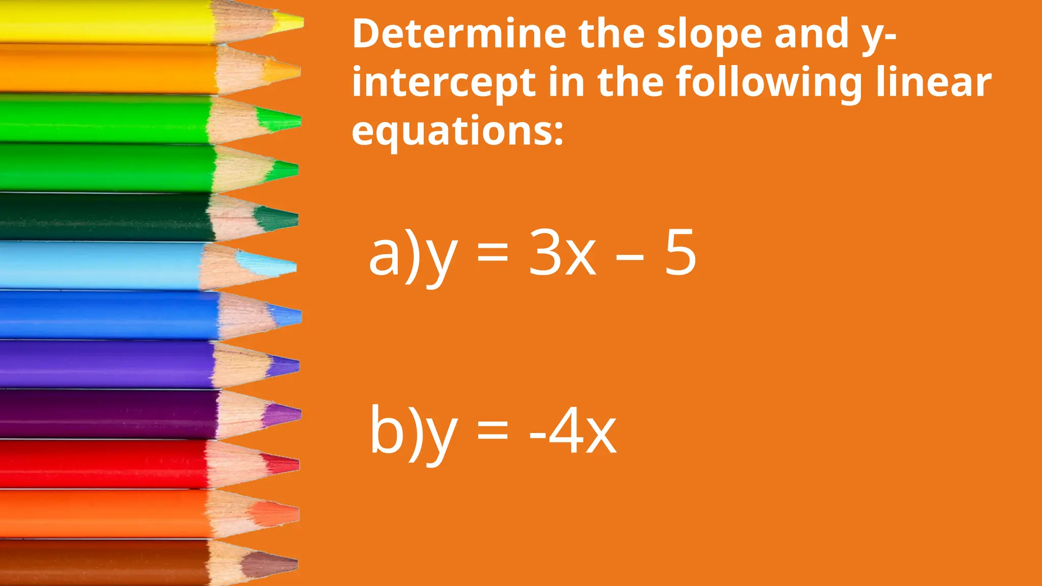
35. Determine the slope and y-
intercept in the following linear
equations:
a)y = 3x – 5
b)y = -4x

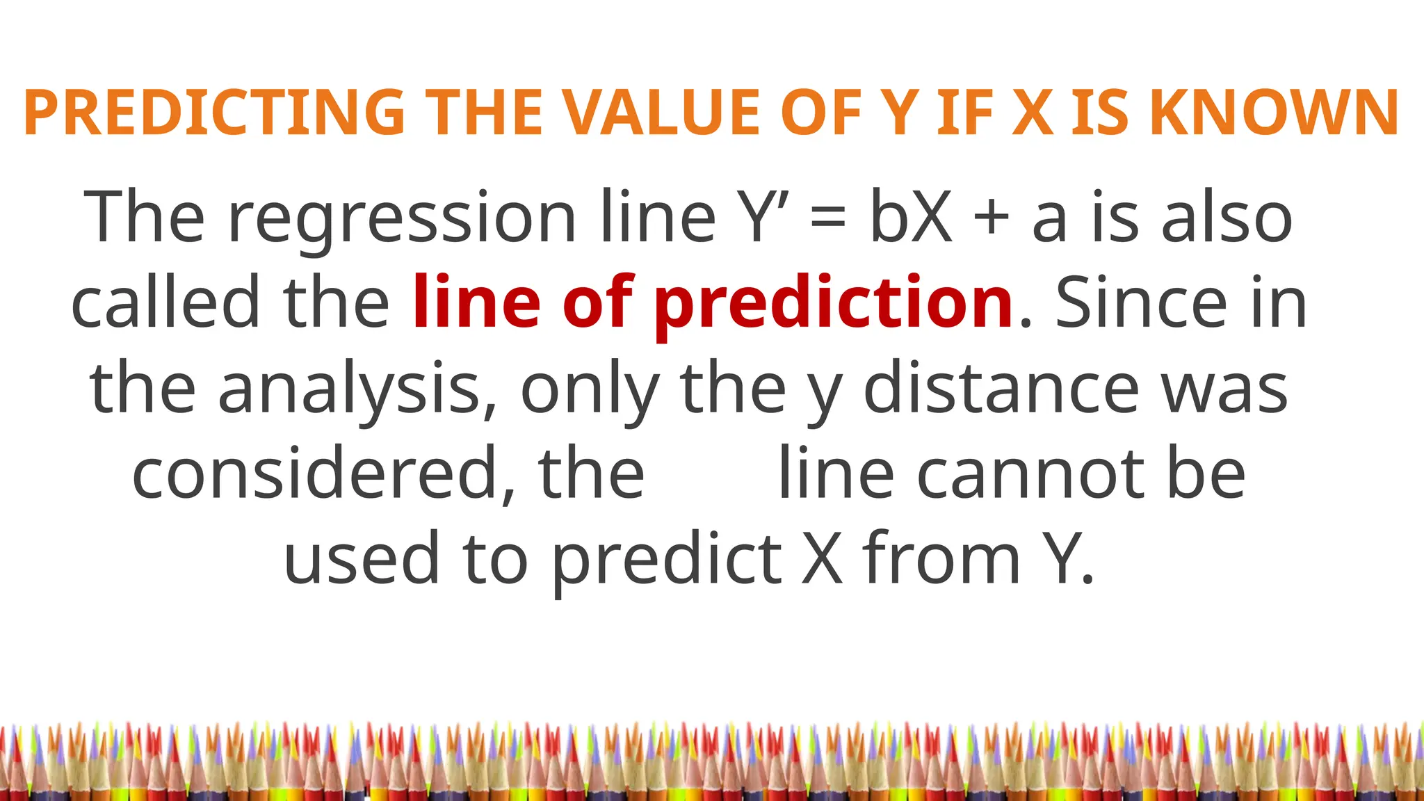
36. PREDICTING THE VALUE OF Y IF X IS KNOWN
The regression line Y’ = bX + a is also
called the line of prediction. Since in
the analysis, only the y distance was
considered, the line cannot be
used to predict X from Y.

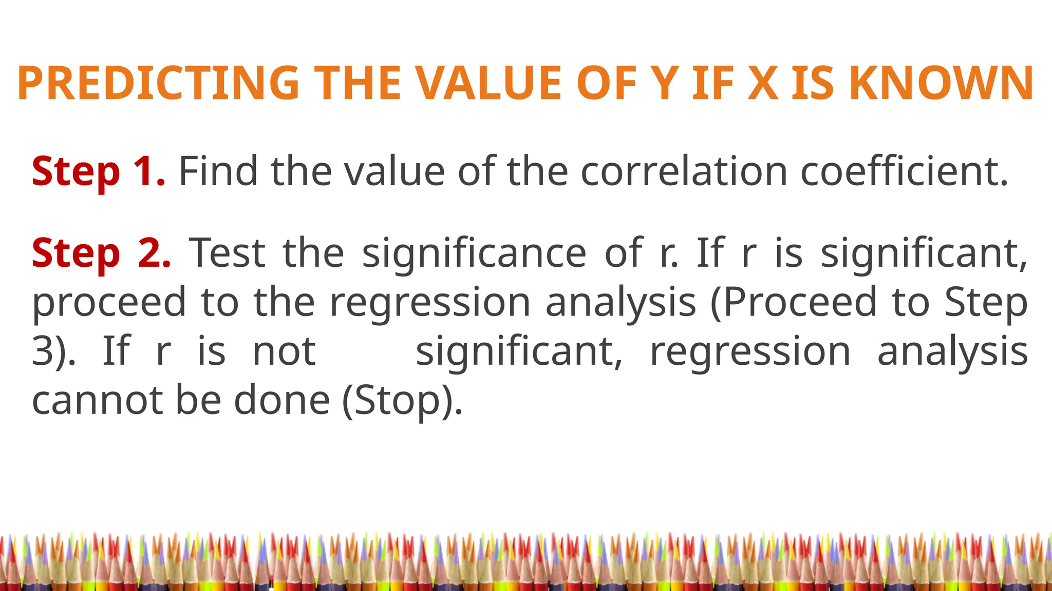
37. PREDICTING THE VALUE OF Y IF X IS KNOWN
Step 1. Find the value of the correlation coefficient.
Step 2. Test the significance of r. If r is significant,
proceed to the regression analysis (Proceed to Step
3). If r is not significant, regression analysis
cannot be done (Stop).

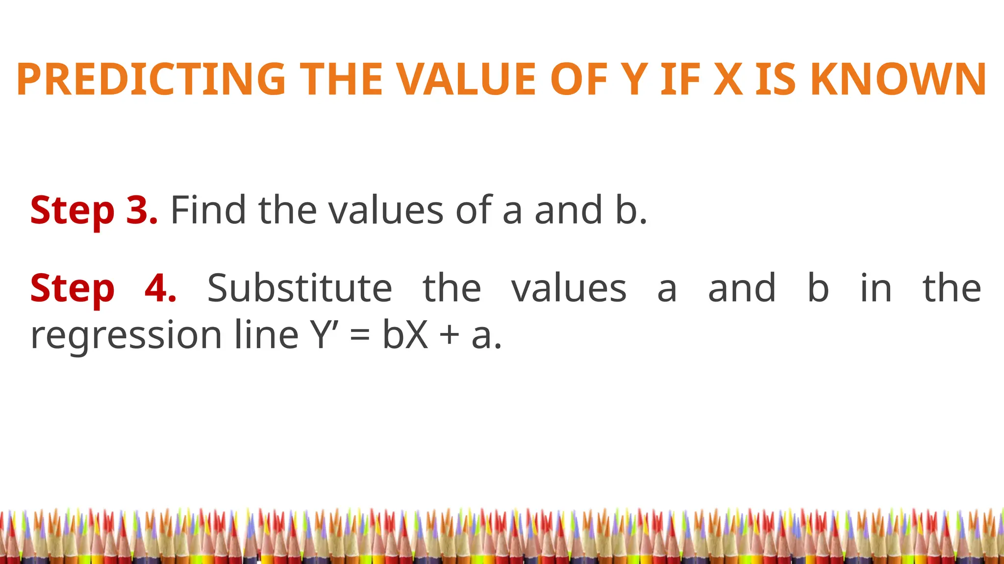
38. PREDICTING THE VALUE OF Y IF X IS KNOWN
Step 3. Find the values of a and b.
Step 4. Substitute the values a and b in the
regression line Y’ = bX + a.

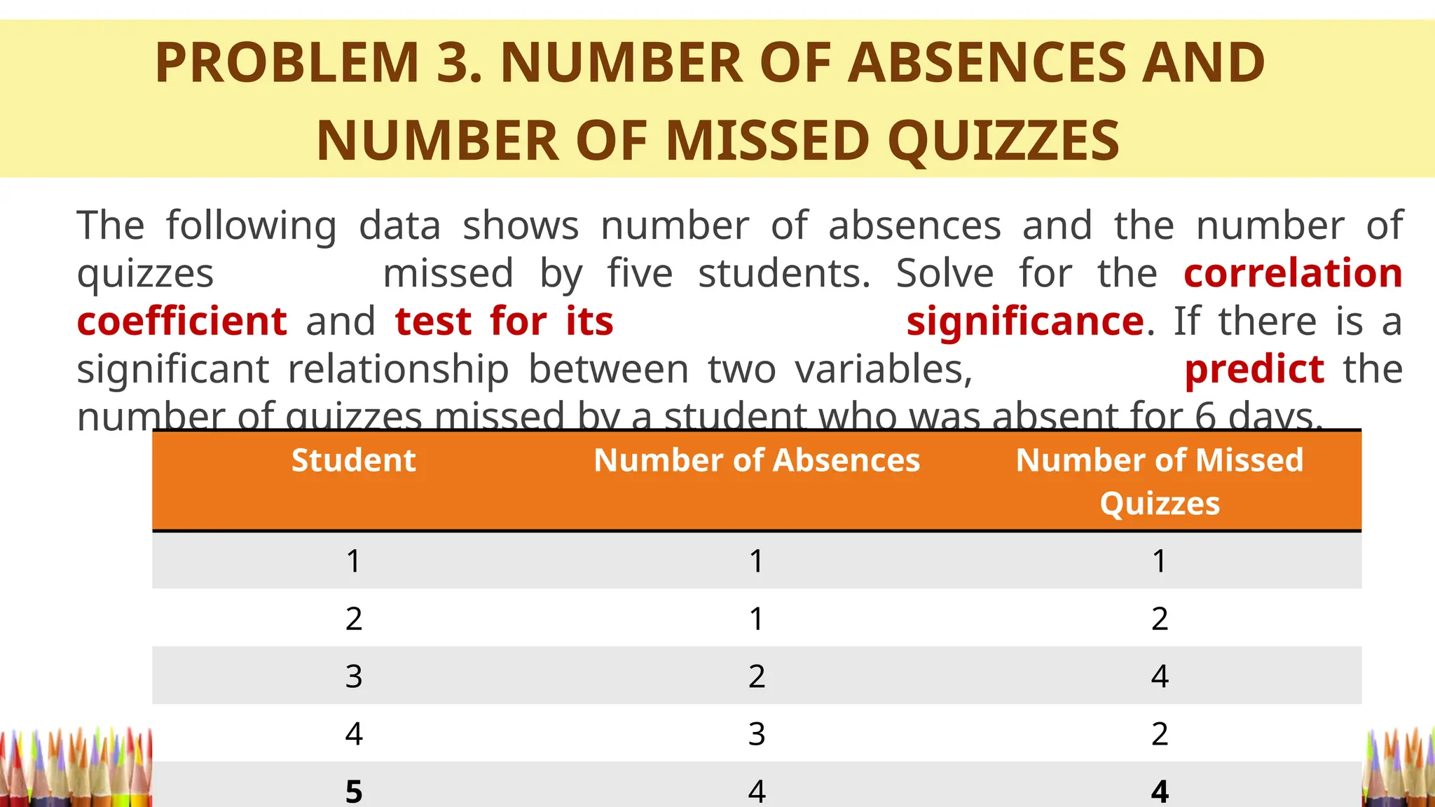
39. PROBLEM 3. NUMBER OF ABSENCES AND
NUMBER OF MISSED QUIZZES
The following data shows number of absences and the number of
quizzes missed by five students. Solve for the correlation
coefficient and test for its significance. If there is a
significant relationship between two variables, predict the
number of quizzes missed by a student who was absent for 6 days.
Student Number of Absences Number of Missed
Quizzes
1 1 1
2 1 2
3 2 4
4 3 2
5 4 4

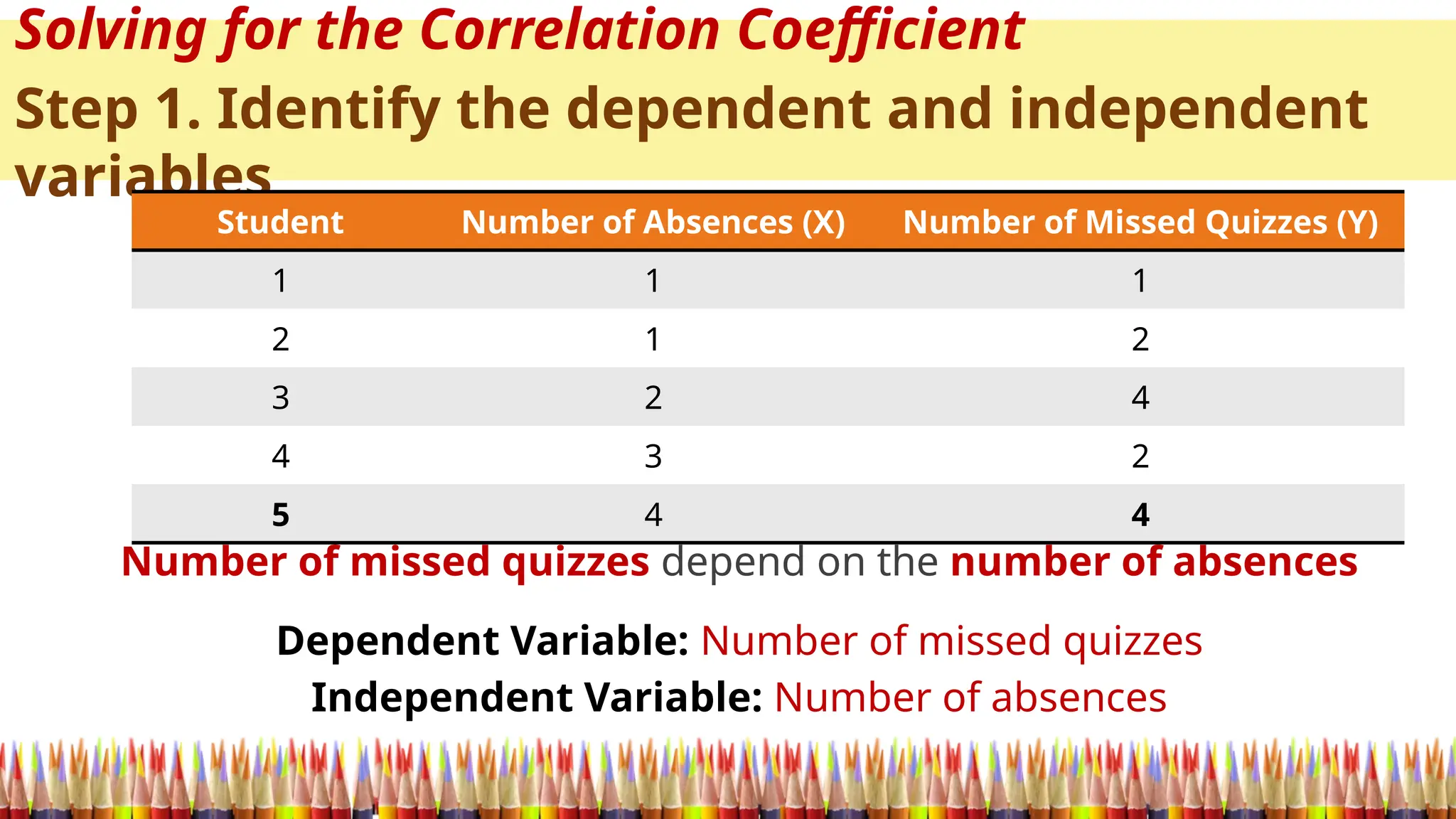
40. Solving for the Correlation Coefficient
Step 1. Identify the dependent and independent
variables
Number of missed quizzes depend on the number of absences
Dependent Variable: Number of missed quizzes
Independent Variable: Number of absences
Student Number of Absences (X) Number of Missed Quizzes (Y)
1 1 1
2 1 2
3 2 4
4 3 2
5 4 4

41. Solving for the Correlation Coefficient
Step 2. Compute for the correlation coefficient
𝑟 =
𝑛∑ 𝑋𝑌 −(∑ 𝑋 )(∑ 𝑌 )
√[𝑛∑ 𝑋2
−(∑ 𝑋 )
2
][𝑛∑ 𝑌 2
−(∑ 𝑌 )
2
]
Student X Y X2
Y2
XY
1 1 1
2 1 2
3 2 4
4 3 2
5 4 4

42. Solving for the Correlation Coefficient
Step 2. Compute for the correlation coefficient
𝑟 =
5(33)−(11)(13)
√[5(31)−(11)
2
][5( 41)−(13)
2
]
Student X Y X2
Y2
XY
1 1 1 1 1 1
2 1 2 1 4 2
3 2 4 4 16 8
4 3 2 9 4 6
5 4 4 16 16 16

43. Solving for the Correlation Coefficient
Step 2. Compute for the correlation coefficient
𝑟=
5(33)−(11)(13)
√[5(31)−(11)
2
][5(41)−(13)
2
]
=
22
√(34)(36)
=𝟎.𝟔𝟑
Student X Y X2
Y2
XY
1 1 1 1 1 1
2 1 2 1 4 2
3 2 4 4 16 8
4 3 2 9 4 6
5 4 4 16 16 16

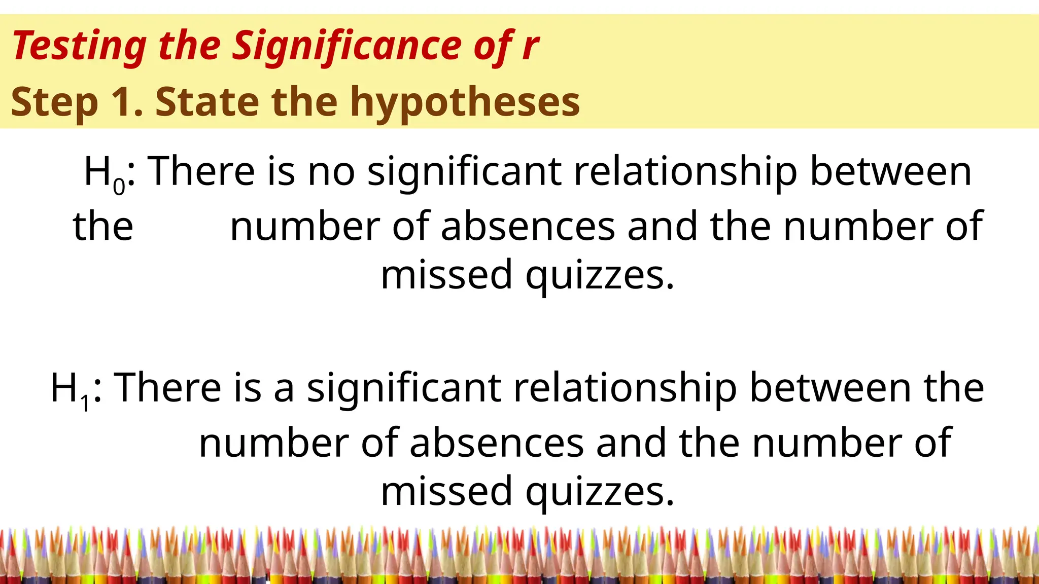
44. Testing the Significance of r
Step 1. State the hypotheses
H0: There is no significant relationship between
the number of absences and the number of
missed quizzes.
H1: There is a significant relationship between the
number of absences and the number of
missed quizzes.

45. Testing the Significance of r
Step 2. Compute for the Value of t
Given: n = 5 r = 0.63

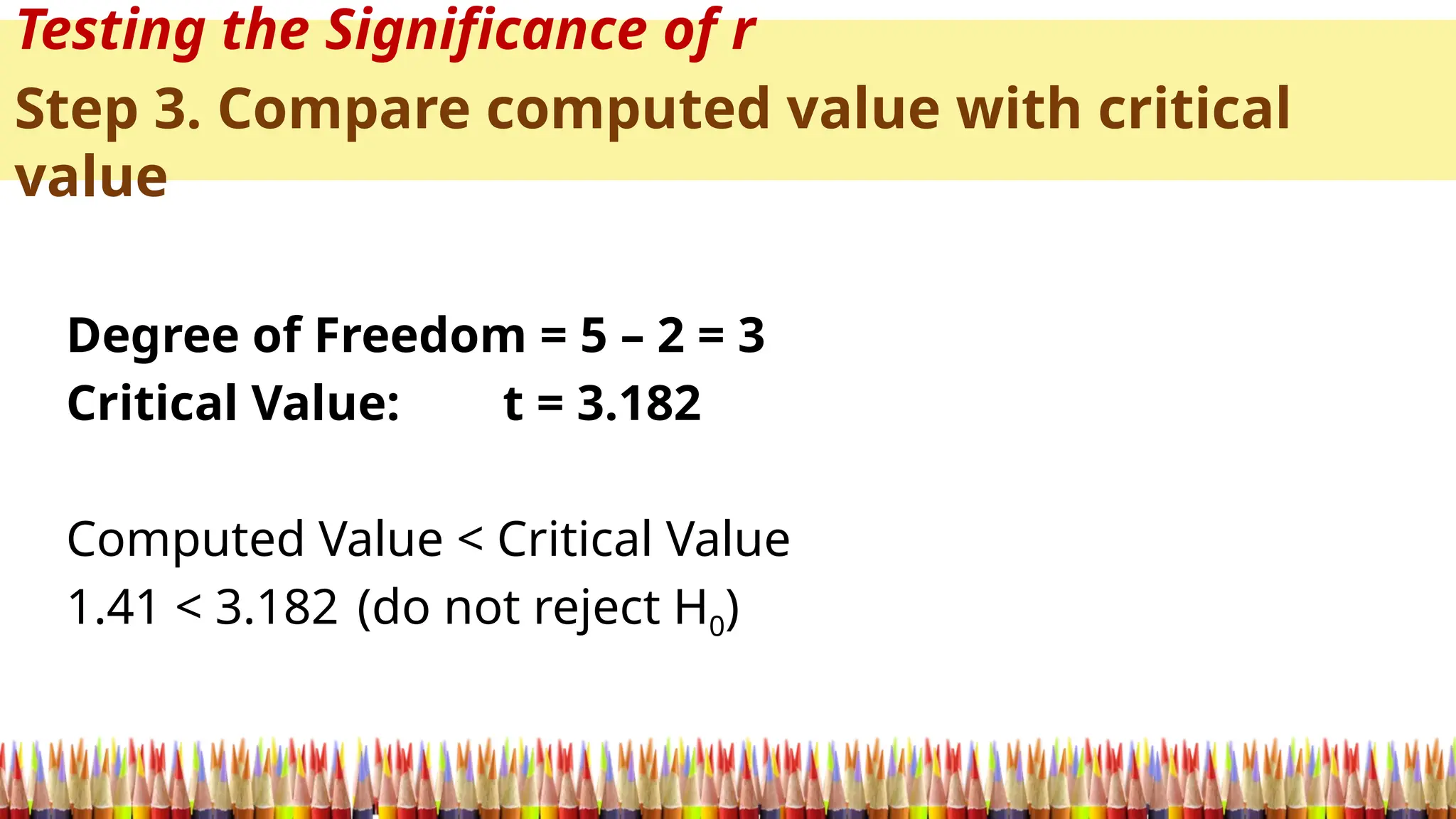
46. Testing the Significance of r
Step 3. Compare computed value with critical
value
Degree of Freedom = 5 – 2 = 3
Critical Value: t = 3.182
Computed Value < Critical Value
1.41 < 3.182 (do not reject H0)

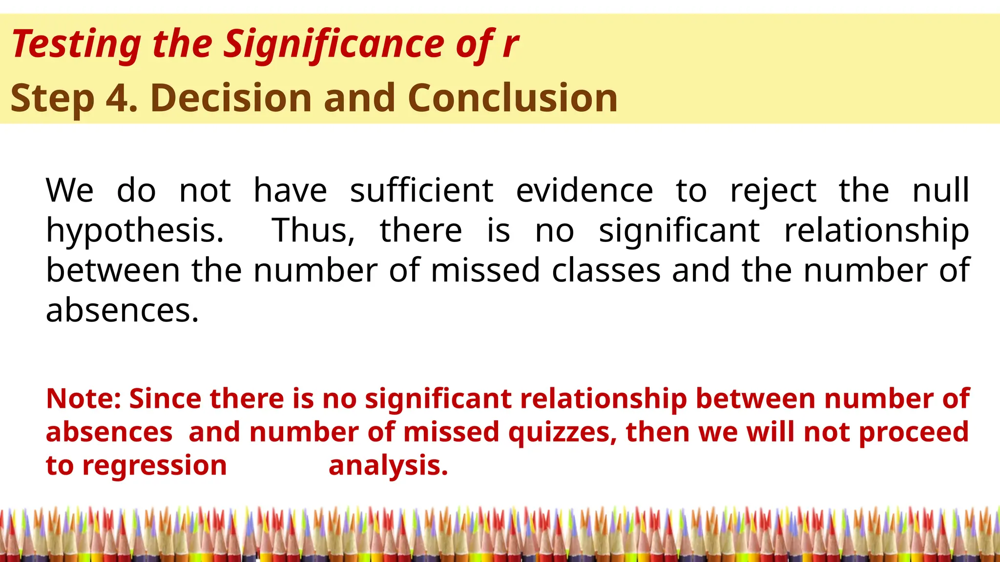
47. Testing the Significance of r
Step 4. Decision and Conclusion
We do not have sufficient evidence to reject the null
hypothesis. Thus, there is no significant relationship
between the number of missed classes and the number of
absences.
Note: Since there is no significant relationship between number of
absences and number of missed quizzes, then we will not proceed
to regression analysis.

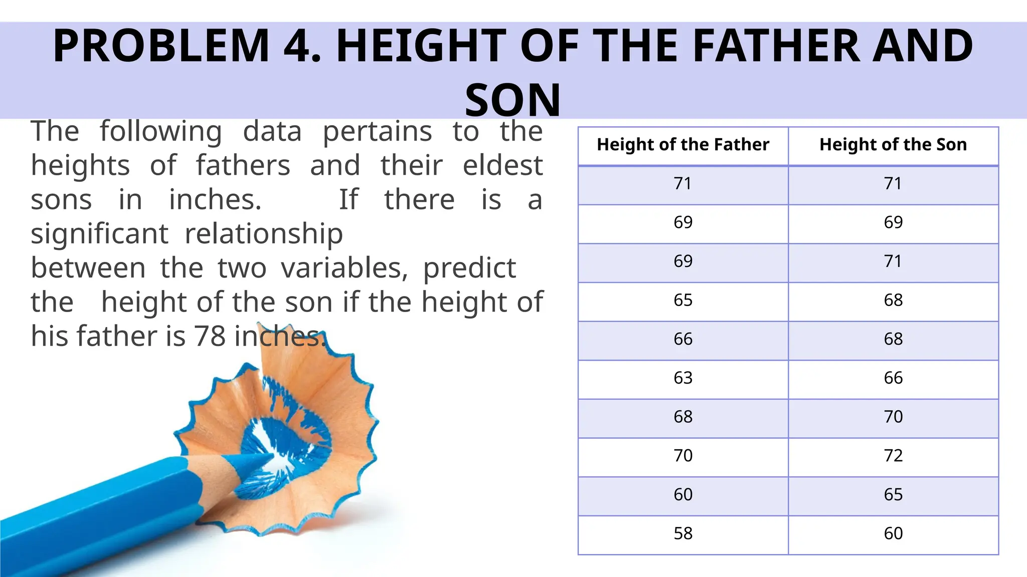
48. PROBLEM 4. HEIGHT OF THE FATHER AND
SON
The following data pertains to the
heights of fathers and their eldest
sons in inches. If there is a
significant relationship
between the two variables, predict
the height of the son if the height of
his father is 78 inches.
Height of the Father Height of the Son
71 71
69 69
69 71
65 68
66 68
63 66
68 70
70 72
60 65
58 60

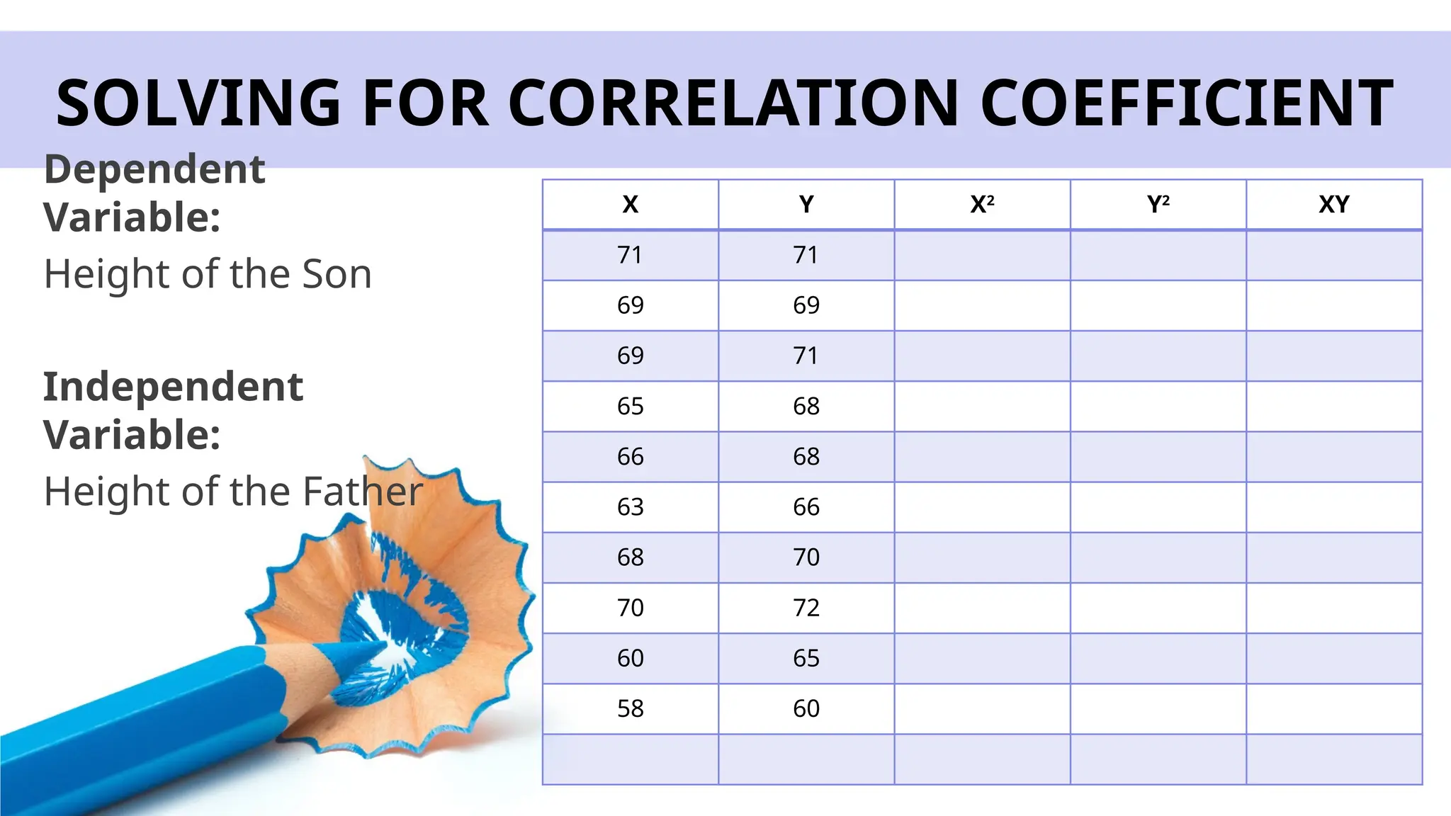
49. SOLVING FOR CORRELATION COEFFICIENT
Dependent
Variable:
Height of the Son
Independent
Variable:
Height of the Father
X Y X2
Y2
XY
71 71
69 69
69 71
65 68
66 68
63 66
68 70
70 72
60 65
58 60

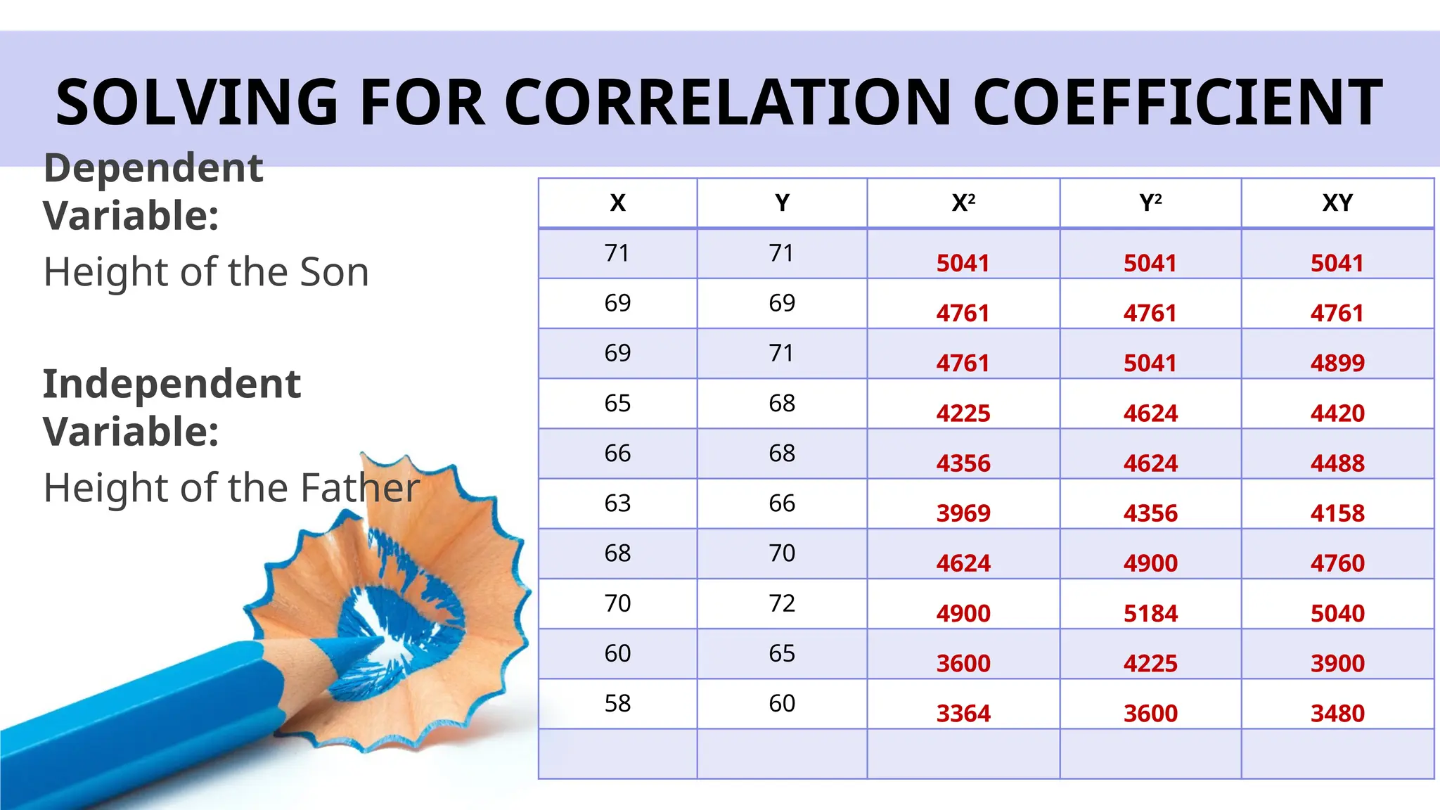
50. SOLVING FOR CORRELATION COEFFICIENT
Dependent
Variable:
Height of the Son
Independent
Variable:
Height of the Father
X Y X2
Y2
XY
71 71 5041 5041 5041
69 69 4761 4761 4761
69 71 4761 5041 4899
65 68 4225 4624 4420
66 68 4356 4624 4488
63 66 3969 4356 4158
68 70 4624 4900 4760
70 72 4900 5184 5040
60 65 3600 4225 3900
58 60 3364 3600 3480

51. SOLVING FOR CORRELATION COEFFICIENT
X Y X2
Y2
XY
71 71 5041 5041 5041
69 69 4761 4761 4761
69 71 4761 5041 4899
65 68 4225 4624 4420
66 68 4356 4624 4488
63 66 3969 4356 4158
68 70 4624 4900 4760
70 72 4900 5184 5040
60 65 3600 4225 3900
58 60 3364 3600 3480
𝑟=
𝑛∑𝑋𝑌−(∑𝑋)(∑𝑌)
√[𝑛∑𝑋
2
−(∑𝑋)
2
][𝑛∑𝑌
2
−(∑𝑌)
2
]

52. SOLVING FOR CORRELATION COEFFICIENT
X Y X2
Y2
XY
71 71 5041 5041 5041
69 69 4761 4761 4761
69 71 4761 5041 4899
65 68 4225 4624 4420
66 68 4356 4624 4488
63 66 3969 4356 4158
68 70 4624 4900 4760
70 72 4900 5184 5040
60 65 3600 4225 3900
58 60 3364 3600 3480
𝑟=
(10)(44,947)−(659)(680)
√[10(43601)−(659)
2
][10(46356)−(680)
2
]
=
1350
√(1729)(1160)
=𝟎.𝟗𝟓

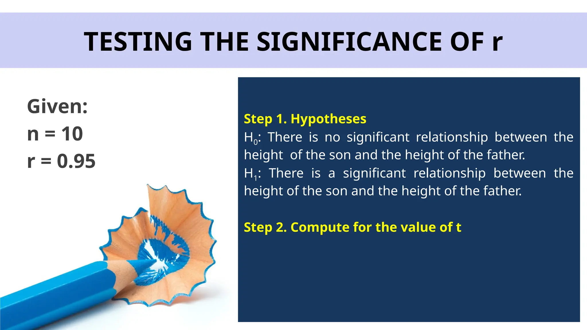
53. TESTING THE SIGNIFICANCE OF r
Given:
n = 10
r = 0.95
Step 1. Hypotheses
H0: There is no significant relationship between the
height of the son and the height of the father.
H1: There is a significant relationship between the
height of the son and the height of the father.
Step 2. Compute for the value of t

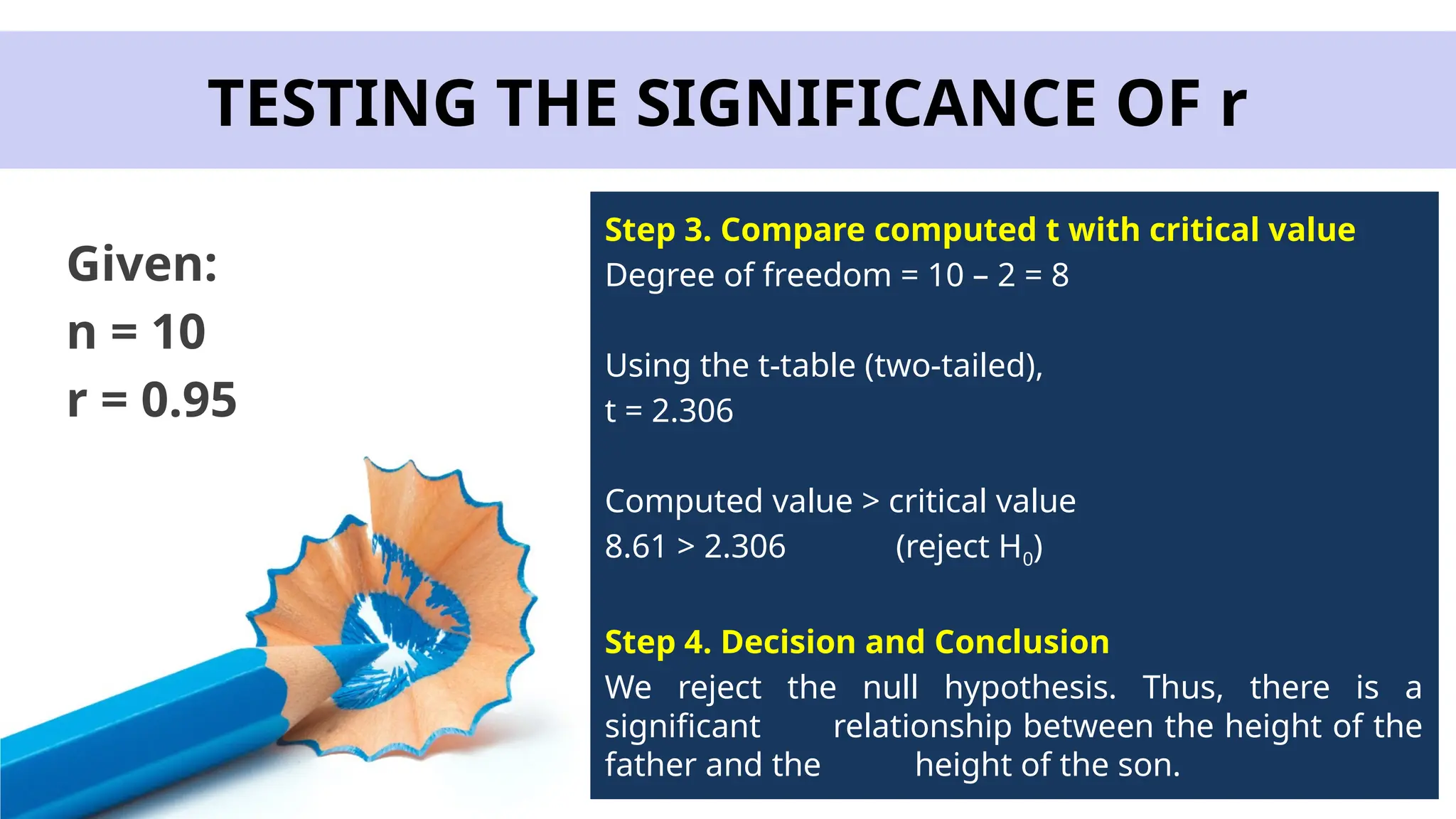
54. TESTING THE SIGNIFICANCE OF r
Given:
n = 10
r = 0.95
Step 3. Compare computed t with critical value
Degree of freedom = 10 – 2 = 8
Using the t-table (two-tailed),
t = 2.306
Computed value > critical value
8.61 > 2.306 (reject H0)
Step 4. Decision and Conclusion
We reject the null hypothesis. Thus, there is a
significant relationship between the height of the
father and the height of the son.

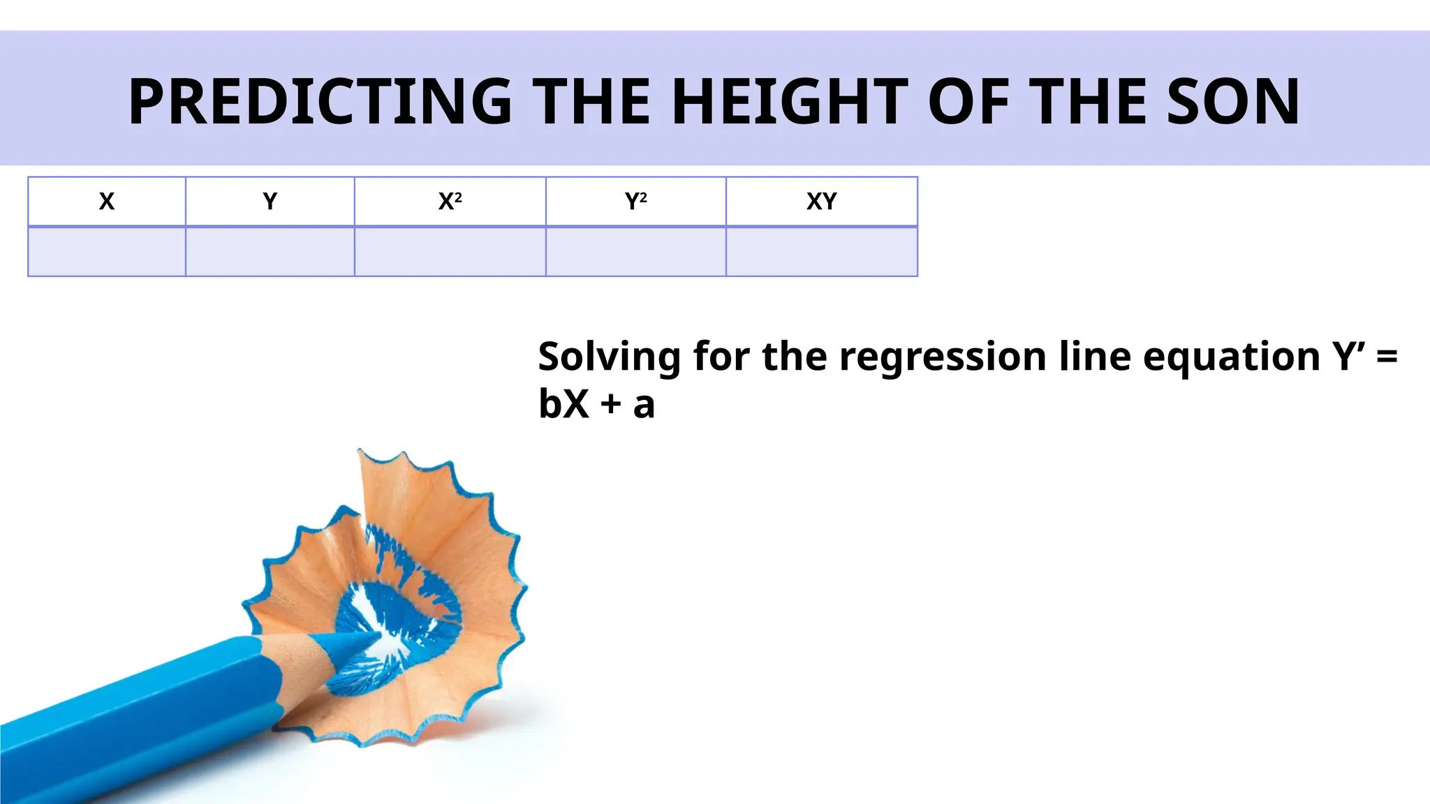
55. PREDICTING THE HEIGHT OF THE SON
Solving for the regression line equation Y’ =
bX + a
X Y X2
Y2
XY

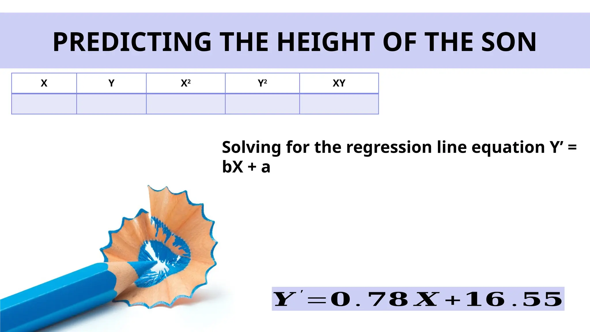
56. PREDICTING THE HEIGHT OF THE SON
Solving for the regression line equation Y’ =
bX + a
X Y X2
Y2
XY
𝒀 ′
=𝟎 . 𝟕𝟖 𝑿 +𝟏𝟔 .𝟓𝟓

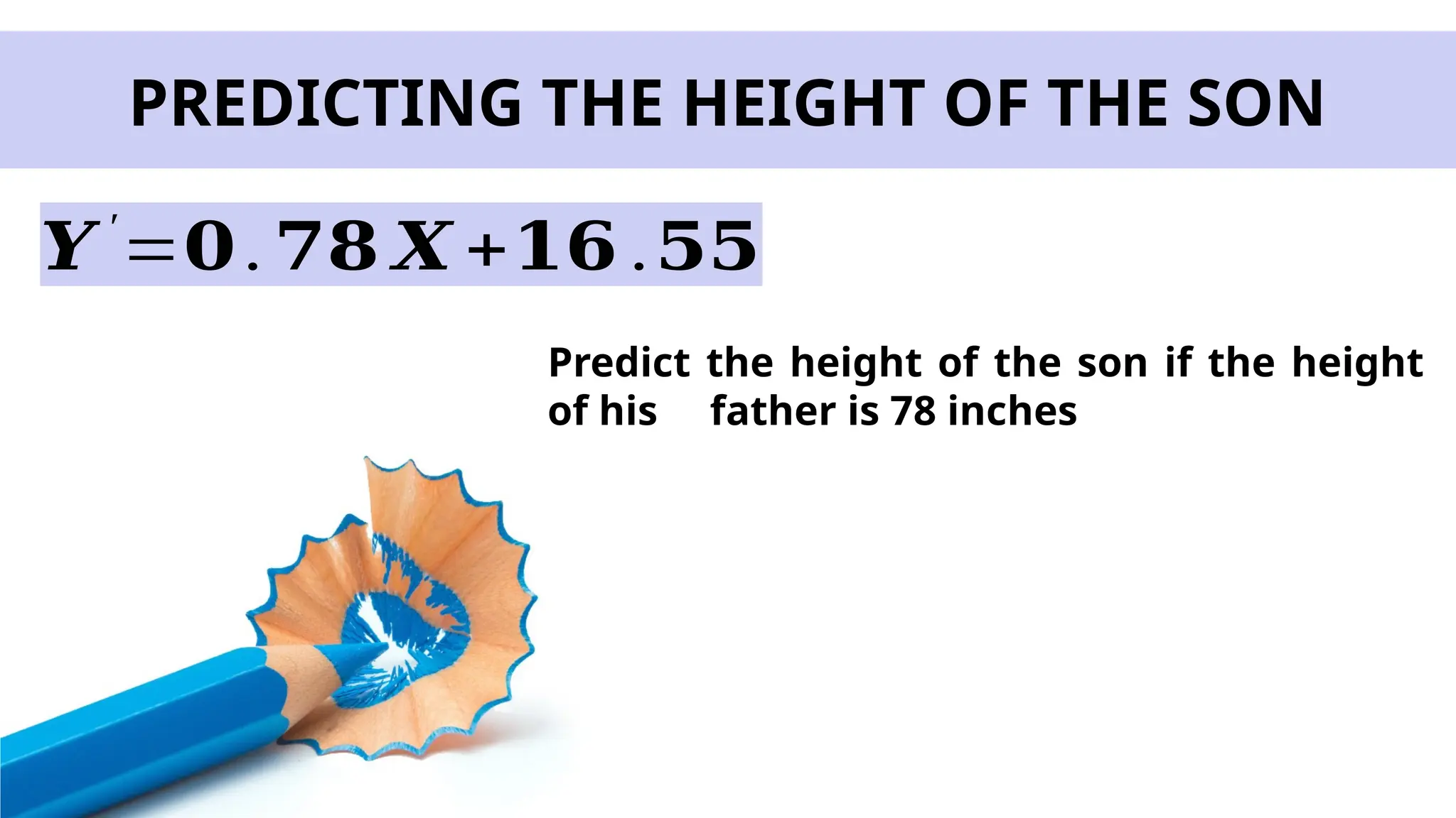
57. PREDICTING THE HEIGHT OF THE SON
Predict the height of the son if the height
of his father is 78 inches
𝒀 ′
=𝟎.𝟕𝟖 𝑿 +𝟏𝟔 .𝟓𝟓

58. EXPLORING THE
REGRESSION ANALYSIS
CHAPTER 6 l LESSON 3 l STATISTICS AND PROBABILITY