SECTION 2
Objectives
After goingthrough this Unit, you should be able to:
Understand the concept of automatic load-frequency control and the dependence of power
system frequency on active (or real) power demand.
Appreciate the measures adopted to control the generation of real power in power plants.
Appreciate the methods used to increase the transmittable real/active power in
transmission lines.
Explain how real power losses in a transmission line can be reduced.
Solve related examples of real power generations in plants and active power flows in lines.
FREQUENCY AND ACTIVE POWER CONTROL –
MAINTENANCE OF REAL POWER BALANCE
3.
SECTION 2
Objectives ofpower systems operation
Objectives of power systems operation
The most important objectives that must be met in the day-to-day operation of a
power grid or the individual power systems that constitute its components are:
1. Maintenance of real power balance
2. Control of frequency
3. Maintenance of reactive power balance
4. Control of voltage profile
5. Maintenance of “optimum” generation schedule (economic dispatch)
6. Maintenance of “optimum” power routing (load flow analysis)
4.
SECTION 2
Objectives ofpower systems operation
It must be stressed that these objectives are to be met in normal system
operation.
Under abnormal or fault or emergency conditions, the effects of the system
disturbances must be minimized.
That is, we wish to operate with maximum security.
The six main objectives of power system operation stated above are not
necessarily mutually exclusive.
5.
SECTION 2
Objectives ofpower systems operation
For example, the automatic control of power system frequency at 50 Hz under
normal state of operation is closely intertwined with the problem of real power
balance.
Hence the term automatic load frequency control (ALFC) describes this joint
task.
No doubt that the ALFC problem is the most basic one that confronts the power
systems engineer.
ALFC facilities are comparatively sophisticated devices which form an
automatic generation control system (AGCS).
6.
SECTION 2
WHY FREQUENCYTENDS TO VARY
The frequency is closely related to the real power balance in the overall network.
Under normal operating conditions, the system generators run synchronously
and generate together the power that at each moment is being drawn by all loads
plus the real transmission system losses.
And so at any point in time, Generation = Demand + Losses
7.
SECTION 2
WHY FREQUENCYTENDS TO VARY
The transmission system losses, amounting usually to a few percent, consists of
1. ohmic losses in the various transmission components
2. corona losses on the lines
3. core losses in transformers and generators
8.
SECTION 2
WHY FREQUENCYTENDS TO VARY
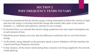
It must be remembered that the electric energy is being transmitted at almost the
velocity of light, and since the energy is not being stored (the storage that
actually takes place in the reactive elements, i.e., inductors and capacitors,
amounts to zero averages.
In electrical form, we conclude that electric energy production rate must equal
consumption rate at each moment of time.
Should the power balance not exist, then the difference would enter into or exist
from kinetic storage.
As the kinetic energy depends on the generator speed, a power imbalance will
thus translate into a speed (and hence frequency) deviation
9.
SECTION 2
WHY FREQUENCYTENDS TO VARY
It must be remembered that the electric energy is being transmitted at almost the velocity of light,
and since the energy is not being stored (the storage that actually takes place in the reactive
elements, i.e., inductors and capacitors, amounts to zero averages.
In electrical form, we conclude that electric energy production rate must equal consumption rate
at each moment of time.
Should the power balance not exist, then the difference would enter into or exist from kinetic
storage.
As the kinetic energy depends on the generator speed, a power imbalance will thus translate into
a speed (and hence frequency) deviation.
In that situation, all the motors which during those moments were being supplied by the network,
would speed up.
10.
SECTION 2
WHY FREQUENCYTENDS TO VARY
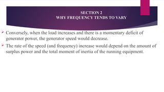
Conversely, when the load increases and there is a momentary deficit of
generator power, the generator speed would decrease.
The rate of the speed (and frequency) increase would depend on the amount of
surplus power and the total moment of inertia of the running equipment.
11.
SECTION 2
AUTOMATIC LOADFREQUENCY CONTROL (ALFC)
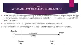
ALFC may play either supplementary or main part in dispatch control, depending on the type
of power systems, transmission capabilities and on the level of coordination concerned with
power exchanges.
To understand the ALFC systems, let us consider a hypothetical case of
a single generator unit supplying power to an isolated load through a transmission line.
12.
SECTION 2
AUTOMATIC LOADFREQUENCY CONTROL (ALFC)
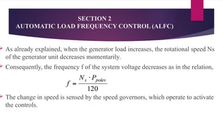
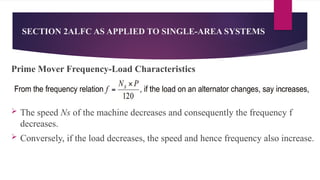
As already explained, when the generator load increases, the rotational speed Ns
of the generator unit decreases momentarily.
Consequently, the frequency f of the system voltage decreases as in the relation,
The change in speed is sensed by the speed governors, which operate to activate
the controls.
13.
SECTION 2
AUTOMATIC LOADFREQUENCY CONTROL (ALFC)
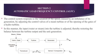
The control system responds to the variation of the speed, caused by an imbalance of its
generation, by adjusting the control valves of a steam turbine or of the opening of the gates of
a hydro-turbine.
In this manner, the input (water or steam) into the turbine is adjusted, thereby restoring the
balance between the turbine output and the unit generation.
14.
SECTION 2
AUTOMATIC LOADFREQUENCY CONTROL (ALFC)
In short, the power output of a generator is changed only by adjusting the mechanical
input to the prime mover (steam turbines, hydro turbines, gas turbines, etc).
The generation-load control or regulation is achieved by measuring the frequency.
A frequency sensor-comparator senses the actual system frequency f and compares it
with a reference frequency ref f (50 Hz). A frequency error signal given by
A transducer amplifies the error signal into an actuating command which is sent on to
the turbine steam valve (or gate, in case of hydro plant).
15.
SECTION 2
AUTOMATIC LOADFREQUENCY CONTROL (ALFC)
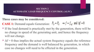
Three cases may be considered:
CASE 1: Demand equals Generation:
If the load demand is practically met by the generation, there will be
no change in speed of the generating unit, and hence the frequency
will not change.
Δf = 0 thus implies the actual system frequency equals the reference
frequency and the demand is well balanced by generation, in which
case no changes will need to be effected in the generation.
16.
SECTION 2
AUTOMATIC LOADFREQUENCY CONTROL (ALFC)
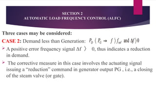
Three cases may be considered:
CASE 2: Demand less than Generation:
A positive error frequency signal Δf 〉 0, thus indicates a reduction
in demand.
The corrective measure in this case involves the actuating signal
issuing a “reduction” command in generator output PG , i.e., a closing
of the steam valve (or gate).
17.
SECTION 2
AUTOMATIC LOADFREQUENCY CONTROL (ALFC)
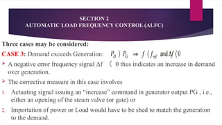
Three cases may be considered:
CASE 3: Demand exceeds Generation:
A negative error frequency signal Δf 〈 0 thus indicates an increase in demand
over generation.
The corrective measure in this case involves
1. Actuating signal issuing an “increase” command in generator output PG , i.e.,
either an opening of the steam valve (or gate) or
2. Importation of power or Load would have to be shed to match the generation
to the demand.
18.
SECTION 2
AUTOMATIC LOADFREQUENCY CONTROL (ALFC)
Some important questions arise in connection with the actual operation
of an ALFC system, such as:
How “responsive” should the control loop be? Clearly, it is not wise to
let the generators “chase” every load excursion, however short it may
be. This would cause unnecessary wear and tear on the equipment.
What generators should participate in the ALFC operation? In a power
system, the ALFC job is delegated to those generators most suitable for
the job.
19.
SECTION 2
AUTOMATIC LOADFREQUENCY CONTROL (ALFC)
It must be noted that, it is much easier to control the power level in a
hydro turbine than in a steam-driven generator.
Consequently, if we have a generation mix, hydro turbines are natural
candidates for the ALFC job.
As noted, the basic role of the ALFC is to maintain a desired
megawatt power output of a generator unit and thus assist in
controlling the frequency of the large system interconnection.
20.
SECTION 2
ALFC ASAPPLIED TO SINGLE-AREA SYSTEMS
The ALFC also helps to keep the net interchange of power between
pool members at predetermined values.
The ALFC loop will maintain control only during normal(that is, small
and slow or steady-state) changes in load and frequency.
It is typically unable to provide adequate control during abnormal (or
emergency) situations, when large megawatt power imbalances occur.
In that situation, more drastic emergency controls must be applied
21.
SECTION 2
ALFC ASAPPLIED TO SINGLE-AREA SYSTEMS
Speed-Governing Control System
This flow increment translates into a turbine power increment
ΔPmech and a corresponding megawatt power increment ΔP in the
generator output.
The position of the valve can be affected via a linkage system either
• directly, by the speed changer or
• indirectly via a feedback mechanism.
22.
SECTION 2
ALFC ASAPPLIED TO SINGLE-AREA SYSTEMS
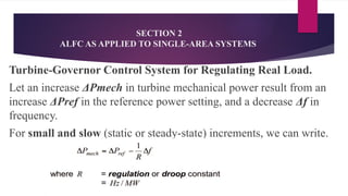
Turbine-Governor Control System for Regulating Real Load.
Let an increase ΔPmech in turbine mechanical power result from an
increase ΔPref in the reference power setting, and a decrease Δf in
frequency.
For small and slow (static or steady-state) increments, we can write.
23.
SECTION 2
ALFC ASAPPLIED TO SINGLE-AREA SYSTEMS
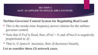
Turbine-Governor Control System for Regulating Real Load.
This is the steady-state frequency power relation for the turbine-
governor control.
Note that if Pref is fixed, then ΔPref = 0, and ΔPmech is negatively
proportional to Δf .
That is, if Δpmech increases, then Δf decreases linearly.
Let us consider three (3) network cases.
24.
SECTION 2
ALFC ASAPPLIED TO SINGLE-AREA SYSTEMS
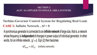
Turbine-Governor Control System for Regulating Real Load.
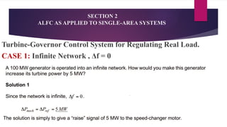
CASE 1: Infinite Network , Δf = 0
25.
SECTION 2
ALFC ASAPPLIED TO SINGLE-AREA SYSTEMS
Turbine-Governor Control System for Regulating Real Load.
CASE 1: Infinite Network , Δf = 0
Example 1
26.
SECTION 2
ALFC ASAPPLIED TO SINGLE-AREA SYSTEMS
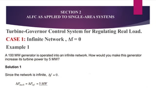
Turbine-Governor Control System for Regulating Real Load.
CASE 1: Infinite Network , Δf = 0
Example 1
27.
SECTION 2
ALFC ASAPPLIED TO SINGLE-AREA SYSTEMS
Turbine-Governor Control System for Regulating Real Load.
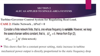
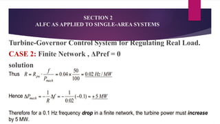
CASE 2: Finite Network , ΔPref = 0
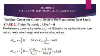
This shows that for a constant power setting, static increase in turbine
mechanical power output is directly proportional to the static frequency drop
28.
SECTION 2
ALFC ASAPPLIED TO SINGLE-AREA SYSTEMS
Turbine-Governor Control System for Regulating Real Load.
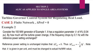
CASE 2: Finite Network , ΔPref = 0
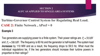
Example 2
solution
29.
SECTION 2
ALFC ASAPPLIED TO SINGLE-AREA SYSTEMS
Turbine-Governor Control System for Regulating Real Load.
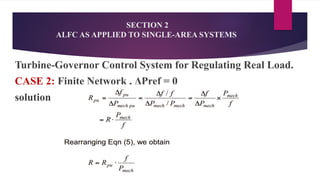
CASE 2: Finite Network , ΔPref = 0
solution
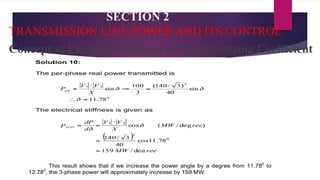
30.
SECTION 2
ALFC ASAPPLIED TO SINGLE-AREA SYSTEMS
Turbine-Governor Control System for Regulating Real Load.
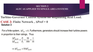
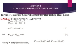
CASE 2: Finite Network , ΔPref = 0
solution
31.
SECTION 2
ALFC ASAPPLIED TO SINGLE-AREA SYSTEMS
Turbine-Governor Control System for Regulating Real Load.
CASE 2: Finite Network , ΔPref = 0
32.
SECTION 2
ALFC ASAPPLIED TO SINGLE-AREA SYSTEMS
Turbine-Governor Control System for Regulating Real Load.
CASE 2: Finite Network , ΔPref = 0
33.
SECTION 2
ALFC ASAPPLIED TO SINGLE-AREA SYSTEMS
Turbine-Governor Control System for Regulating Real Load.
CASE 2: Finite Network , ΔPref = 0
34.
SECTION 2
ALFC ASAPPLIED TO SINGLE-AREA SYSTEMS
Turbine-Governor Control System for Regulating Real Load.
CASE 2: Finite Network , ΔPref = 0
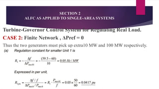
Thus the two generators must pick up extra10 MW and 100 MW respectively.
35.
SECTION 2
ALFC ASAPPLIED TO SINGLE-AREA SYSTEMS
Turbine-Governor Control System for Regulating Real Load.
CASE 2: Finite Network , ΔPref = 0
NOTES:
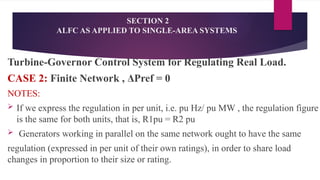
If we express the regulation in per unit, i.e. pu Hz/ pu MW , the regulation figure
is the same for both units, that is, R1pu = R2 pu
Generators working in parallel on the same network ought to have the same
regulation (expressed in per unit of their own ratings), in order to share load
changes in proportion to their size or rating.
36.
SECTION 2
ALFC ASAPPLIED TO SINGLE-AREA SYSTEMS
Turbine-Governor Control System for Regulating Real Load.
CASE 2: Finite Network , ΔPref = 0
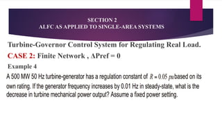
Example 4
37.
SECTION 2
ALFC ASAPPLIED TO SINGLE-AREA SYSTEMS
Turbine-Governor Control System for Regulating Real Load.
CASE 2: Finite Network , ΔPref = 0
38.
SECTION 2
ALFC ASAPPLIED TO SINGLE-AREA SYSTEMS
Turbine-Governor Control System for Regulating Real Load.
CASE 3: Changes Occur in Both Reference Power Setting and
Frequency
39.
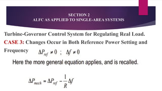
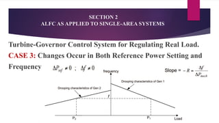
Turbine-Governor Control Systemfor Regulating Real Load.
CASE 3: Changes Occur in Both Reference Power Setting and
Frequency
SECTION 2
ALFC AS APPLIED TO SINGLE-AREA SYSTEMS
40.
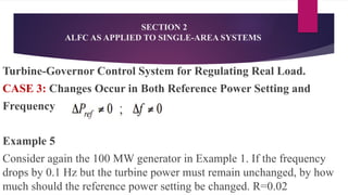
Turbine-Governor Control Systemfor Regulating Real Load.
CASE 3: Changes Occur in Both Reference Power Setting and
Frequency
Example 5
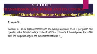
Consider again the 100 MW generator in Example 1. If the frequency
drops by 0.1 Hz but the turbine power must remain unchanged, by how
much should the reference power setting be changed. R=0.02
SECTION 2
ALFC AS APPLIED TO SINGLE-AREA SYSTEMS
41.
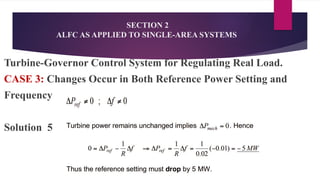
SECTION 2
ALFC ASAPPLIED TO SINGLE-AREA SYSTEMS
Turbine-Governor Control System for Regulating Real Load.
CASE 3: Changes Occur in Both Reference Power Setting and
Frequency
Solution 5
42.
SECTION 2ALFC ASAPPLIED TO SINGLE-AREA SYSTEMS
Prime Mover Frequency-Load Characteristics
The speed Ns of the machine decreases and consequently the frequency f
decreases.
Conversely, if the load decreases, the speed and hence frequency also increase.
43.
SECTION 2ALFC ASAPPLIED TO SINGLE-AREA SYSTEMS
Prime Mover Frequency-Load Characteristics
The speed-power characteristic is thus similar to the frequency-power
characteristic.
This type of characteristic where an increase in the load leads to a decrease in
speed or frequency is known as drooping characteristic.
All practical prime movers have drooping speed-power characteristics.
44.
SECTION 2
ALFC ASAPPLIED TO SINGLE-AREA SYSTEMS
Prime Mover Frequency-Load Characteristics
45.
SECTION 2
ALFC ASAPPLIED TO SINGLE-AREA SYSTEMS
Prime Mover Frequency-Load Characteristics
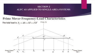
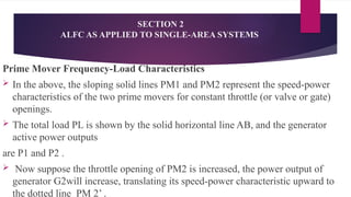
In the above, the sloping solid lines PM1 and PM2 represent the speed-power
characteristics of the two prime movers for constant throttle (or valve or gate)
openings.
The total load PL is shown by the solid horizontal line AB, and the generator
active power outputs
are P1 and P2 .
Now suppose the throttle opening of PM2 is increased, the power output of
generator G2will increase, translating its speed-power characteristic upward to
the dotted line PM 2’ .
46.
SECTION 2
ALFC ASAPPLIED TO SINGLE-AREA SYSTEMS
Prime Mover Frequency-Load Characteristics
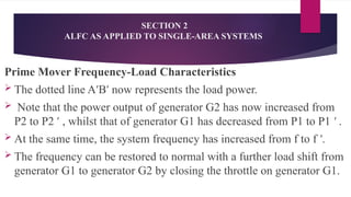
The dotted line A B now represents the load power.
ʹ ʹ
Note that the power output of generator G2 has now increased from
P2 to P2 , whilst that of generator G1 has decreased from P1 to P1 .
ʹ ʹ
At the same time, the system frequency has increased from f to f .
ʹ
The frequency can be restored to normal with a further load shift from
generator G1 to generator G2 by closing the throttle on generator G1.
47.
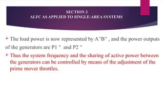
The loadpower is now represented by A B , and the power outputs
ʹʹ ʹʹ
of the generators are P1 and P2
ʺ ʺ
Thus the system frequency and the sharing of active power between
the generators can be controlled by means of the adjustment of the
prime mover throttles.
SECTION 2
ALFC AS APPLIED TO SINGLE-AREA SYSTEMS
48.
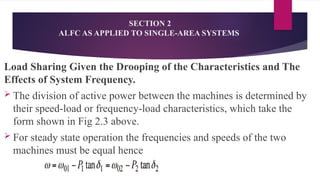
Load Sharing Giventhe Drooping of the Characteristics and The
Effects of System Frequency.
The division of active power between the machines is determined by
their speed-load or frequency-load characteristics, which take the
form shown in Fig 2.3 above.
For steady state operation the frequencies and speeds of the two
machines must be equal hence
SECTION 2
ALFC AS APPLIED TO SINGLE-AREA SYSTEMS
49.
SECTION 2
ALFC ASAPPLIED TO SINGLE-AREA SYSTEMS
Load Sharing Given the Drooping of the Characteristics and The
Effects of System Frequency.
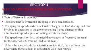
The slope tanδ is termed the drooping of the characteristics.
Changing the speed-load characteristic changes the load sharing, and this
involves an alteration to the governor setting (speed changer setting
affects ω and speed regulation setting affects the slope).
The speed regulation is so adjusted that changes in frequency are small
(of the order of 5 % from no load to full load).
Unless the speed–load characteristics are identical, the machines can
never share the total load in accordance with their ratings
50.
SECTION 2
ALFC ASAPPLIED TO SINGLE-AREA SYSTEMS
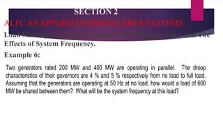
Load Sharing Given the Drooping of the Characteristics and The
Effects of System Frequency.
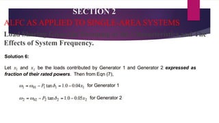
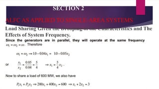
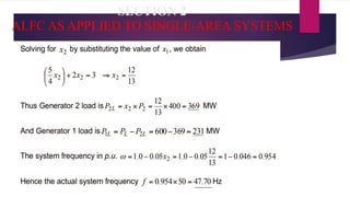
Example 6:
51.
SECTION 2
ALFC ASAPPLIED TO SINGLE-AREA SYSTEMS
Load Sharing Given the Drooping of the Characteristics and The
Effects of System Frequency.
52.
SECTION 2
ALFC ASAPPLIED TO SINGLE-AREA SYSTEMS
Load Sharing Given the Drooping of the Characteristics and The
Effects of System Frequency.
SECTION 2
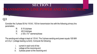
TRANSMISSION LINEPOWER AND ITS CONTROL
Transmission lines permit us to dispatch surpluses of power from one grid
bus to another.
They constitute important network links that make it possible to choose
alternate power flow configurations for optimum economy and security.
In this section, we wish to study the factors that affect the line power flows,
and particularly, how we go about controlling these flows.
First, let us remind ourselves of how power lines are modelled
55.
SECTION 2
TRANSMISSION LINEPOWER AND ITS CONTROL
First, let us remind ourselves of how power lines are modelled
LINE PARAMETERS
A three-phase transmission line is mostly used in overhead design.
In dense urban areas, underground cables are often used when overhead lines would represent unacceptable
safety hazards.
Typically, the bare stranded conductors consist of a steel core for mechanical
strength and an outer current-carrying shell made of aluminium.
To obtain a more flexible conductor, both the steel and aluminium portions are designed stranded.
56.
SECTION 2
TRANSMISSION LINEPOWER AND ITS CONTROL
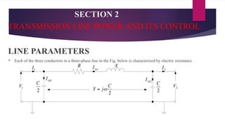
LINE PARAMETERS
Each of the three conductors in a three-phase line in the Fig. below is characterized by electric resistance.
57.
SECTION 2
TRANSMISSION LINEPOWER AND ITS CONTROL
LINE PARAMETERS
The current in each conductor surrounds itself with a magnetic field, resulting in a self-
inductance.
In addition to the self-inductance per phase, there is also a mutual inductance
between phases.
Finally, there exist electric capacitances between each conductor, and these are equivalent
to a set of capacitances between each phase and a neutral node.
In addition to capacitances between phases, there also exists a capacitance between each
phase and ground.
58.
SECTION 2
TRANSMISSION LINEPOWER AND ITS CONTROL
LINE PARAMETERS
And so electrically, the transmission line is characterized by circuit parameters in the form of both series
and shunt elements.
Clearly, the line resistance belongs to the series elements; so does the self-inductance caused by the
magnetic flux surrounding each conductor.
The capacitance that exists between the conductors represents a shunt or parallel
admittance.
There is also a shunt resistance which represents the leakage current along insulator strings, but for normal
weather conditions, the leakage current can be usually neglected. All the above circuit parameters are
distributed in nature.
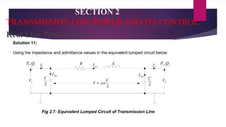
The total effect of these distributed parameters can be shown to be equivalent to that of the lumped circuit
shown above.
59.
SECTION 2
TRANSMISSION LINEPOWER AND ITS CONTROL
LINE PARAMETERS
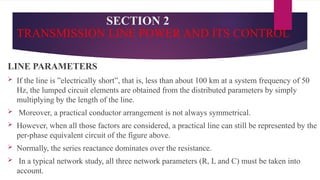
If the line is ”electrically short”, that is, less than about 100 km at a system frequency of 50
Hz, the lumped circuit elements are obtained from the distributed parameters by simply
multiplying by the length of the line.
Moreover, a practical conductor arrangement is not always symmetrical.
However, when all those factors are considered, a practical line can still be represented by the
per-phase equivalent circuit of the figure above.
Normally, the series reactance dominates over the resistance.
In a typical network study, all three network parameters (R, L and C) must be taken into
account.
60.
SECTION 2
TRANSMISSION LINEPOWER AND ITS CONTROL
LINE PARAMETERS
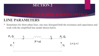
Sometimes for short urban lines, one may disregard both the resistance and capacitance and
work with the simplified line model shown below.
SECTION 2
TRANSMISSION LINEPOWER AND ITS CONTROL
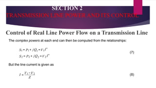
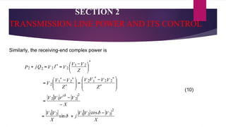
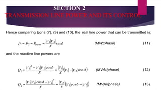
The following deductions must be noted:
The real line power flow on a transmission line depends on the magnitude and
direction on the difference in phase angles between the end-point voltage phasors.
The power magnitude increases with phase difference, and the flow direction is
from the leading to the lagging voltage.
The voltages and reactances must be given in per-phase values to yield the per-
phase values of power.
Because the line resistance was neglected, the real line powers at each end are
equal.
SECTION 2
TRANSMISSION LINEPOWER AND ITS CONTROL
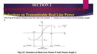
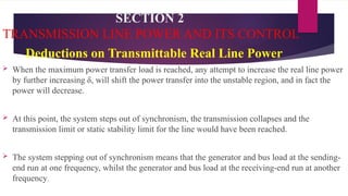
Deductions on Transmittable Real Line Power
When the maximum power transfer load is reached, any attempt to increase the real line power
by further increasing δ, will shift the power transfer into the unstable region, and in fact the
power will decrease.
At this point, the system steps out of synchronism, the transmission collapses and the
transmission limit or static stability limit for the line would have been reached.
The system stepping out of synchronism means that the generator and bus load at the sending-
end run at one frequency, whilst the generator and bus load at the receiving-end run at another
frequency.
SECTION 2
TRANSMISSION LINEPOWER AND ITS CONTROL
Deductions on Transmittable Real Line Power
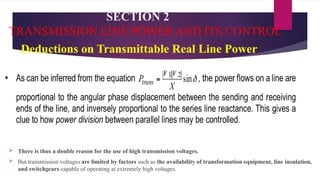
A positive sin δ , that is, V1 leading V2 , results in megawatt flow in direction left to right,
i.e., from the sending-end to the receiving-end.
But if the power angle δ increases in a negative sense (V2 leading V1), the power becomes
negative, that is, power is transmitted in the reverse direction from right to left, i.e., from the
receiving-end to the sending-end.
• In short, the real power flow is from the point with the most leading angle to the point with the
most lagging angle, whilst VAR flow is from the higher voltage on a line to the lower voltage.
SECTION 2
TRANSMISSION LINEPOWER AND ITS CONTROL
Deductions on Transmittable Real Line Power
Following a power system disturbance, oscillations occur, during which
generating machines’ power angles increase and decrease within a period
determined by the inertia of the machines connected to the line.
In such cases, the swings produced by a disturbance may cause the angular
displacement of a line to exceed the stability limit on heavily loaded lines.
This factor is also considered in establishing the loading limits of transmission
lines.
76.
SECTION 2
TRANSMISSION LINEPOWER AND ITS CONTROL
Deductions on Transmittable Real Line Power
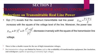
There is thus a double reason for the use of high transmission voltages.
But transmission voltages are limited by factors such as the availability of transformation equipment, line insulation,
and switchgears capable of operating at extremely high voltages.
77.
SECTION 2
TRANSMISSION LINEPOWER AND ITS CONTROL
Deductions on Transmittable Real Line Power
There is thus a double reason for the use of high transmission voltages.
But transmission voltages are limited by factors such as the availability of transformation equipment, line insulation,
and switchgears capable of operating at extremely high voltages.
78.
SECTION 2
TRANSMISSION LINEPOWER AND ITS CONTROL
Deductions on Transmittable Real Line Power
If a long transmission line with greater power-handling capability and higher impedance is
paralleled with a short transmission line with low load capability, the load will divide
inversely proportional to the impedances of the line.
Consequently, the short line with low load-handling capability may overload before the
capacity of the larger line is reached.
If the voltage on the high-impedance line is increased or decreased (by means of, say, a
voltage regulator), the load division will not be affected, but increased VAR flows will result,
with their attendant losses.
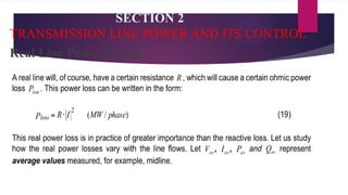
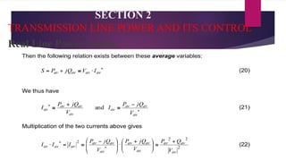
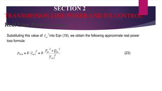
SECTION 2
TRANSMISSION LINEPOWER AND ITS CONTROL
Deductions from Real Line Power Loss
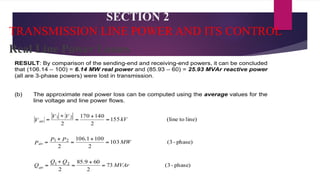
This formula is important, because it reveals that the real and reactive line power flows contribute to the real power losses.
From the point of view of power loss, one should therefore minimize the reactive line flow.
The real line power losses are proportional to the sum of the squares of the real and reactive line flows and inversely
proportional to the voltage magnitude square.
In practice, the minimization of reactive power flow in the line is accomplished by generation of the reactive power at the
bus where it is needed.
If no generator is available (and it must be remembered that an overexcited generator generates reactive power), then one
often installs shunt capacitors for this purpose.
SECTION 2
TRANSMISSION LINEPOWER AND ITS CONTROL
VOLTAGE AND FREQUENCY DEPENDENCY OF LOAD
An important feature characterising all loads is their dependency on voltage and frequency.
During faults and other abnormal situations, the voltage may vary greatly, resulting in major load fluctuations.
Even minor changes in voltage and frequency can cause load changes of practical significance.
We shall discuss two important load types, impedance loads and motor loads.
98.
SECTION 2
TRANSMISSION LINEPOWER AND ITS CONTROL
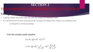
Voltage Dependency of Impedance Loads
Lighting, heaters and similar loads fall under the category of impedance loads.
It is desired to know by how many percent the real load will change if the voltage on an impedance load
is changed by a certain percentage.
99.
SECTION 2
TRANSMISSION LINEPOWER AND ITS CONTROL
Voltage Dependency of Impedance Loads
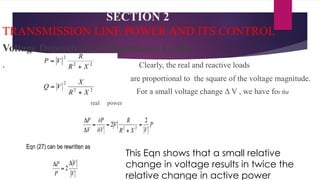
. Clearly, the real and reactive loads
are proportional to the square of the voltage magnitude.
For a small voltage change Δ V , we have for the
real power
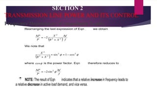
This Eqn shows that a small relative
change in voltage results in twice the
relative change in active power
100.
SECTION 2
TRANSMISSION LINEPOWER AND ITS CONTROL
Frequency Dependency of Impedance Loads
The reactance depends on the frequency f according to the relation
X = 2 πfl. Thus from the Eqn above, we have