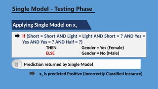
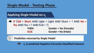
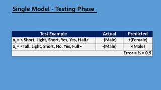
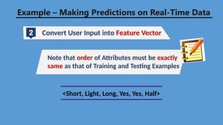
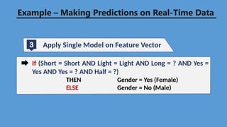
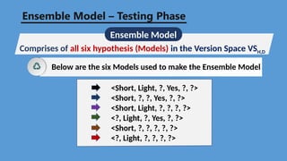
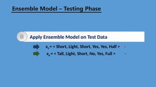
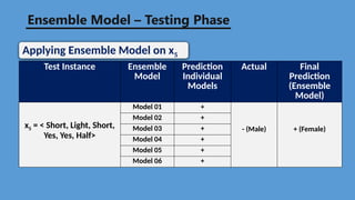
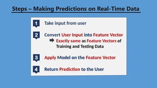
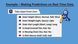
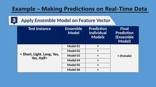
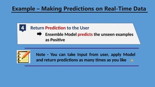
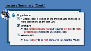
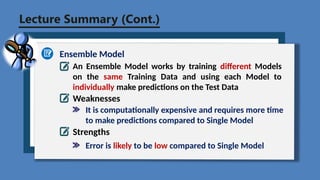
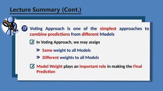
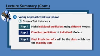
ِ‫م‬ْ‫ي‬ِ‫ح‬َّ‫ر‬‫ال‬ ِ‫ن‬ٰ‫م‬ْ‫ح‬َّ‫ر‬‫ال‬ ِ‫هللا‬ ِ‫م‬ْ‫س‬ِ‫ب‬
Machine Learning
Dr. Rao Muhammad Adeel Nawab
Slides Credits:
Lecture 04: Version Space Algorithm
Dr. Allah Bux Sargana
Edited By:
Version Space
Single Model
Approach
Single Model = <Short, Light, ?, Yes, ?, ?>
Apply Single Model on Test Data
Randomly select a Single Model form VSH,D
x5 = < Short, Light, Short, Yes, Yes, Half > -
x6 = < Tall, Light, Short, No, Yes, Full > -
Single Model - Testing Phase
Applying Single Model on x5
If (Short = Short AND Light = Light AND Short = ? AND Yes =
Yes AND Yes = ? AND Half = ?)
THEN Gender = Yes (Female)
ELSE Gender = No (Male)
x5 is predicted Positive (Incorrectly Classified Instance)
Prediction returned by Single Model
Single Model - Testing Phase
Applying Single Model on x6
If (Tall = Short AND Light = Light AND Short = ? AND No =
Yes AND Yes = ? AND Full = ?)
THEN Gender = Yes (Female)
ELSE Gender = No (Male)
x6 is predicted Negative (Correctly Classified Instance)
Prediction returned by Single Model
Single Model - Testing Phase
Test Example Actual Predicted
x5 = < Short, Light, Short, Yes, Yes, Half> -(Male) +(Female)
x6 = <Tall, Light, Short, No, Yes, Full> -(Male) -(Male)
Error = ½ = 0.5
Single Model - Testing Phase
Performed well on large Test Data and can be
deployed in Real-world
Single Model is deployed in the Real-world and
now we can make
We assume that our Single Model
Predictions on Real-time Data
Single Model - Application Phase
Steps – Making Predictions on Real-Time Data
1 Take input from User
Convert User Input into Feature Vector
Exactly same as Feature Vectors of
Training and Testing Data
Apply Model on the Feature Vector
Return Prediction to the User
2
3
4
Example – Making Predictions on Real-Time Data
1 Take input from User
Enter Height (Short, Normal, Tall): Short
Enter Weight (Light, Heavy): Light
Enter Hair Length (Short, Long): Long
Is Head Covered (Yes, No): Yes
Is Wearing Chain (Yes, No): Yes
Is Shirt Sleeves (Half, Full): Half
Example – Making Predictions on Real-Time Data
2 Convert User Input into Feature Vector
Note that order of Attributes must be exactly
same as that of Training and Testing Examples
<Short, Light, Long, Yes, Yes, Half>
If (Short = Short AND Light = Light AND Long = ? AND Yes =
Yes AND Yes = ? AND Half = ?)
THEN Gender = Yes (Female)
ELSE Gender = No (Male)
Example – Making Predictions on Real-Time Data
3 Apply Single Model on Feature Vector
4 Return Prediction to the User
Positive
Example – Making Predictions on Real-Time Data
Note - You can take Input from user, apply Model
and return predictions as many times as you like
Domain Experts
Users
Take Feedback on your deployed Single Model from
Improve your Single Model based on Feedback
Single Model - Feedback Phase
Ensemble Model
Approach
Ensemble Model
Comprises of all six hypothesis (Models) in the Version Space VSH,D
Ensemble Model – Testing Phase
Below are the six Models used to make the Ensemble Model
<Short, Light, ?, Yes, ?, ?>
<Short, ?, ?, Yes, ?, ?>
<Short, Light, ?, ?, ?, ?>
<?, Light, ?, Yes, ?, ?>
<Short, ?, ?, ?, ?, ?>
<?, Light, ?, ?, ?, ?>
Apply Ensemble Model on Test Data
x5 = < Short, Light, Short, Yes, Yes, Half > -
x6 = < Tall, Light, Short, No, Yes, Full > -
Ensemble Model – Testing Phase
Test Instance Ensemble
Model
Prediction
Individual
Models
Actual Final
Prediction
(Ensemble
Model)
x5 = < Short, Light, Short,
Yes, Yes, Half>
Model 01 +
- (Male) + (Female)
Model 02 +
Model 03 +
Model 04 +
Model 05 +
Model 06 +
Applying Ensemble Model on x5
Ensemble Model – Testing Phase
Prediction returned by Ensemble Model
x5 is predicted Positive (Incorrectly
Classified Instance)
Final Prediction was calculated based on
Majority Vote
Ensemble Model – Testing Phase
Test Instance Ensemble
Model
Prediction
Individual
Models
Actual Final
Prediction
(Ensemble
Model)
x6 = < Tall, Light, Short,
No, Yes, Full>
Model 01 -
- (Male) - (Male)
Model 02 -
Model 03 -
Model 04 -
Model 05 -
Model 06 +
Applying Ensemble Model on x6
Ensemble Model – Testing Phase
Prediction returned by Ensemble Model
x6 is predicted Negative (Correctly
Classified Instance)
Final Prediction was calculated based on
Majority Vote
Ensemble Model – Testing Phase
Test Example Actual Predicted
x5 = < Short, Light, Short, Yes, Yes, Half> -(Male) +(Female)
x6 = <Tall, Light, Short, No, Yes, Full> -(Male) +(Female)
Error = ½ = 0.5
Ensemble Model – Testing Phase
Performed well on large Test Data and can be
deployed in Real-world
Ensemble Model is deployed in the Real-world and
now we can make
We assume that our Ensemble Model
Predictions on Real-time Data
Ensemble Model – Application Phase
Steps – Making Predictions on Real-Time Data
1 Take input from user
Convert User Input into Feature Vector
Exactly same as Feature Vectors of
Training and Testing Data
Apply Model on the Feature Vector
Return Prediction to the User
2
3
4
Example – Making Predictions on Real-Time Data
1 Take input from User
Enter Height (Short, Normal, Tall): Short
Enter Weight (Light, Heavy): Light
Enter Hair Length (Short, Long): Long
Is Head Covered (Yes, No): Yes
Is Wearing Chain (Yes, No): Yes
Is Shirt Sleeves (Half, Full): Half
Example – Making Predictions on Real-Time Data
2 Convert User Input into Feature Vector
Note that order of Attributes must be exactly
same as that of Training and Testing Examples
<Short, Light, Long, Yes, Yes, Half>
Test Instance Ensemble
Model
Prediction
Individual
Models
Final
Prediction
(Ensemble
Model)
< Short, Light, Long, Yes,
Yes, Half>
Model 01 +
+ (Female)
Model 02 +
Model 03 +
Model 04 +
Model 05 +
Model 06 +
Example – Making Predictions on Real-Time Data
3 Apply Ensemble Model on Feature Vector
Example – Making Predictions on Real-Time Data
Note - Final Prediction was calculated based
on Majority Vote
4 Return Prediction to the User
Ensemble Model predicts the unseen examples
as Positive
Example – Making Predictions on Real-Time Data
Note - You can take Input from user, apply Model
and return predictions as many times as you like
Domain Experts
Users
Take Feedback on your deployed Ensemble Model from
Improve your Ensemble Model based on Feedback
Ensemble Model – Feedback Phase
Discussion – Candidate
Elimination Algorithm
Inductive Bias – Candidate Elimination Algorithm
Inductive Bias
Inductive Bias is the set of assumptions needed in addition to
Training Examples to justify Deductively Learner’s Classification
Inductive Bias of List Candidate
Elimination Algorithm
Training data is error free
Target Function / Concept is present in the Hypothesis
Space (H)
Lecture Summary (Cont.)
List Then Eliminate Algorithm – Summary
Representation of Example
Attribute-Value Pair
Representation of Hypothesis (h)
Conjunction (AND) of Constraints on Attributes
Training Regime
Incremental Method
Lecture Summary (Cont.)
Inductive Bias of List Ten Eliminate Algorithm
Training Data is error-free
Strengths
List Then Eliminate Algorithm overcomes the
limitation of FIND-S Algorithm and
Target Function / Concept is present in the Hypothesis
Space (H)
returns multiple hypothesis, which best fits the Training
Data i.e. Version Space (VSH,D)
Lecture Summary (Cont.)
Weaknesses
Only works on error-free Data
However, Real-world Data is noisy
Works on assumption that Target Function is present in the
Hypothesis Space (H)
However, we may / may not find the Target Function in the
Hypothesis Space (H) and this may / may not be known
List Then Eliminate Algorithm is computationally expensive
because it makes a
pairwise comparison of each Training Example with all
hypothesis in Hypothesis Space (H)
Lecture Summary (Cont.)
List Then Eliminate Algorithm is computationally expensive
because
Hypothesis Space (H) is represented as a List, which forces
To reduce the computational cost of Version Space
Algorithms
Have a more compact representation of Hypothesis Space
(H)
for e.g. Candidate Elimination Algorithm
List Then Eliminate Algorithm to make pairwise
comparisons
Lecture Summary (Cont.)
Candidate Elimination Algorithm – Summary
Representation of Example
Attribute-Value Pair
Representation of Hypothesis (h)
Conjunction (AND) of Constraints on Attributes
Training Regime
Incremental Method
Lecture Summary (Cont.)
Inductive Bias of Candidate Elimination Algorithm
Training Data is error-free
Strengths
Candidate Elimination Algorithm overcomes the limitation
of List Then Eliminate Algorithm and
Target Function / Concept is present in the Hypothesis
Space (H)
provides a more compact representation of the Version
Space
Lecture Summary (Cont.)
Version Space returned by Candidate Elimination Algorithm
can be used to make predictions on unseen Data using
either a
Single Model or
Ensemble Model
Weaknesses
Only works on error-free Data
However, Real-world Data is noisy
Works on assumption that Target Function is present in the
Hypothesis Space (H)
However, we may / may not find the Target Function in the
Hypothesis Space (H) and this may / may not be known
Lecture Summary (Cont.)
Only works when values of Attributes are Categorical
However, in Real-world many Machine Learning Problems
have
Attributes / Features with Numeric values
Only works for simple representations of Data
However, in Real-world many Machine Learning Problems
have complex representation (for e.g. Face Detection, Face
Recognition etc.)
Lecture Summary (Cont.)
Single Model
A Single Model is trained on the Training Data and used to
make predictions on the Test Data
Strengths
Weaknesses
It is computationally fast and requires less time to make
predictions compared to Ensemble Model
Error is likely to be high compared to Ensemble Model
Lecture Summary (Cont.)
Ensemble Model
An Ensemble Model works by training different Models
on the same Training Data and using each Model to
individually make predictions on the Test Data
Weaknesses
Strengths
It is computationally expensive and requires more time
to make predictions compared to Single Model
Error is likely to be low compared to Single Model
Lecture Summary (Cont.)
Voting Approach is one of the simplest approaches to
combine predictions from different Models
In Voting Approach, we may assign
Same weight to all Models
Model Weight plays an important role in making the Final
Prediction
Different weights to all Models
Lecture Summary (Cont.)
Voting Approach works as follows
Step 1 Make individual predictions using different Models
Step 2 Combine predictions of individual Models
Step 3 Final Prediction of x will be the class which has
the majority vote
Given a Test instance x
Lecture Summary (Cont.)
Voting Classifier is not an actual Classifier (Machine
Learning Algorithm) but a wrapper for a set of different
Machine Learning Algorithms, which are trained and
tested on the same Data
A Voting Classifier combines predictions of individual
Machine Learning Algorithms to make Final Predictions on
unseen Data

Lecture06_Version Space Algorithm Part2.pptx

  • 1.
  • 2.
    Machine Learning Dr. RaoMuhammad Adeel Nawab Slides Credits: Lecture 04: Version Space Algorithm Dr. Allah Bux Sargana Edited By:
  • 3.
  • 4.
  • 5.
    Single Model =<Short, Light, ?, Yes, ?, ?> Apply Single Model on Test Data Randomly select a Single Model form VSH,D x5 = < Short, Light, Short, Yes, Yes, Half > - x6 = < Tall, Light, Short, No, Yes, Full > - Single Model - Testing Phase
  • 6.
    Applying Single Modelon x5 If (Short = Short AND Light = Light AND Short = ? AND Yes = Yes AND Yes = ? AND Half = ?) THEN Gender = Yes (Female) ELSE Gender = No (Male) x5 is predicted Positive (Incorrectly Classified Instance) Prediction returned by Single Model Single Model - Testing Phase
  • 7.
    Applying Single Modelon x6 If (Tall = Short AND Light = Light AND Short = ? AND No = Yes AND Yes = ? AND Full = ?) THEN Gender = Yes (Female) ELSE Gender = No (Male) x6 is predicted Negative (Correctly Classified Instance) Prediction returned by Single Model Single Model - Testing Phase
  • 8.
    Test Example ActualPredicted x5 = < Short, Light, Short, Yes, Yes, Half> -(Male) +(Female) x6 = <Tall, Light, Short, No, Yes, Full> -(Male) -(Male) Error = ½ = 0.5 Single Model - Testing Phase
  • 9.
    Performed well onlarge Test Data and can be deployed in Real-world Single Model is deployed in the Real-world and now we can make We assume that our Single Model Predictions on Real-time Data Single Model - Application Phase
  • 10.
    Steps – MakingPredictions on Real-Time Data 1 Take input from User Convert User Input into Feature Vector Exactly same as Feature Vectors of Training and Testing Data Apply Model on the Feature Vector Return Prediction to the User 2 3 4
  • 11.
    Example – MakingPredictions on Real-Time Data 1 Take input from User Enter Height (Short, Normal, Tall): Short Enter Weight (Light, Heavy): Light Enter Hair Length (Short, Long): Long Is Head Covered (Yes, No): Yes Is Wearing Chain (Yes, No): Yes Is Shirt Sleeves (Half, Full): Half
  • 12.
    Example – MakingPredictions on Real-Time Data 2 Convert User Input into Feature Vector Note that order of Attributes must be exactly same as that of Training and Testing Examples <Short, Light, Long, Yes, Yes, Half>
  • 13.
    If (Short =Short AND Light = Light AND Long = ? AND Yes = Yes AND Yes = ? AND Half = ?) THEN Gender = Yes (Female) ELSE Gender = No (Male) Example – Making Predictions on Real-Time Data 3 Apply Single Model on Feature Vector
  • 14.
    4 Return Predictionto the User Positive Example – Making Predictions on Real-Time Data Note - You can take Input from user, apply Model and return predictions as many times as you like
  • 15.
    Domain Experts Users Take Feedbackon your deployed Single Model from Improve your Single Model based on Feedback Single Model - Feedback Phase
  • 16.
  • 17.
    Ensemble Model Comprises ofall six hypothesis (Models) in the Version Space VSH,D Ensemble Model – Testing Phase Below are the six Models used to make the Ensemble Model <Short, Light, ?, Yes, ?, ?> <Short, ?, ?, Yes, ?, ?> <Short, Light, ?, ?, ?, ?> <?, Light, ?, Yes, ?, ?> <Short, ?, ?, ?, ?, ?> <?, Light, ?, ?, ?, ?>
  • 18.
    Apply Ensemble Modelon Test Data x5 = < Short, Light, Short, Yes, Yes, Half > - x6 = < Tall, Light, Short, No, Yes, Full > - Ensemble Model – Testing Phase
  • 19.
    Test Instance Ensemble Model Prediction Individual Models ActualFinal Prediction (Ensemble Model) x5 = < Short, Light, Short, Yes, Yes, Half> Model 01 + - (Male) + (Female) Model 02 + Model 03 + Model 04 + Model 05 + Model 06 + Applying Ensemble Model on x5 Ensemble Model – Testing Phase
  • 20.
    Prediction returned byEnsemble Model x5 is predicted Positive (Incorrectly Classified Instance) Final Prediction was calculated based on Majority Vote Ensemble Model – Testing Phase
  • 21.
    Test Instance Ensemble Model Prediction Individual Models ActualFinal Prediction (Ensemble Model) x6 = < Tall, Light, Short, No, Yes, Full> Model 01 - - (Male) - (Male) Model 02 - Model 03 - Model 04 - Model 05 - Model 06 + Applying Ensemble Model on x6 Ensemble Model – Testing Phase
  • 22.
    Prediction returned byEnsemble Model x6 is predicted Negative (Correctly Classified Instance) Final Prediction was calculated based on Majority Vote Ensemble Model – Testing Phase
  • 23.
    Test Example ActualPredicted x5 = < Short, Light, Short, Yes, Yes, Half> -(Male) +(Female) x6 = <Tall, Light, Short, No, Yes, Full> -(Male) +(Female) Error = ½ = 0.5 Ensemble Model – Testing Phase
  • 24.
    Performed well onlarge Test Data and can be deployed in Real-world Ensemble Model is deployed in the Real-world and now we can make We assume that our Ensemble Model Predictions on Real-time Data Ensemble Model – Application Phase
  • 25.
    Steps – MakingPredictions on Real-Time Data 1 Take input from user Convert User Input into Feature Vector Exactly same as Feature Vectors of Training and Testing Data Apply Model on the Feature Vector Return Prediction to the User 2 3 4
  • 26.
    Example – MakingPredictions on Real-Time Data 1 Take input from User Enter Height (Short, Normal, Tall): Short Enter Weight (Light, Heavy): Light Enter Hair Length (Short, Long): Long Is Head Covered (Yes, No): Yes Is Wearing Chain (Yes, No): Yes Is Shirt Sleeves (Half, Full): Half
  • 27.
    Example – MakingPredictions on Real-Time Data 2 Convert User Input into Feature Vector Note that order of Attributes must be exactly same as that of Training and Testing Examples <Short, Light, Long, Yes, Yes, Half>
  • 28.
    Test Instance Ensemble Model Prediction Individual Models Final Prediction (Ensemble Model) <Short, Light, Long, Yes, Yes, Half> Model 01 + + (Female) Model 02 + Model 03 + Model 04 + Model 05 + Model 06 + Example – Making Predictions on Real-Time Data 3 Apply Ensemble Model on Feature Vector
  • 29.
    Example – MakingPredictions on Real-Time Data Note - Final Prediction was calculated based on Majority Vote
  • 30.
    4 Return Predictionto the User Ensemble Model predicts the unseen examples as Positive Example – Making Predictions on Real-Time Data Note - You can take Input from user, apply Model and return predictions as many times as you like
  • 31.
    Domain Experts Users Take Feedbackon your deployed Ensemble Model from Improve your Ensemble Model based on Feedback Ensemble Model – Feedback Phase
  • 32.
  • 33.
    Inductive Bias –Candidate Elimination Algorithm Inductive Bias Inductive Bias is the set of assumptions needed in addition to Training Examples to justify Deductively Learner’s Classification Inductive Bias of List Candidate Elimination Algorithm Training data is error free Target Function / Concept is present in the Hypothesis Space (H)
  • 34.
    Lecture Summary (Cont.) ListThen Eliminate Algorithm – Summary Representation of Example Attribute-Value Pair Representation of Hypothesis (h) Conjunction (AND) of Constraints on Attributes Training Regime Incremental Method
  • 35.
    Lecture Summary (Cont.) InductiveBias of List Ten Eliminate Algorithm Training Data is error-free Strengths List Then Eliminate Algorithm overcomes the limitation of FIND-S Algorithm and Target Function / Concept is present in the Hypothesis Space (H) returns multiple hypothesis, which best fits the Training Data i.e. Version Space (VSH,D)
  • 36.
    Lecture Summary (Cont.) Weaknesses Onlyworks on error-free Data However, Real-world Data is noisy Works on assumption that Target Function is present in the Hypothesis Space (H) However, we may / may not find the Target Function in the Hypothesis Space (H) and this may / may not be known List Then Eliminate Algorithm is computationally expensive because it makes a pairwise comparison of each Training Example with all hypothesis in Hypothesis Space (H)
  • 37.
    Lecture Summary (Cont.) ListThen Eliminate Algorithm is computationally expensive because Hypothesis Space (H) is represented as a List, which forces To reduce the computational cost of Version Space Algorithms Have a more compact representation of Hypothesis Space (H) for e.g. Candidate Elimination Algorithm List Then Eliminate Algorithm to make pairwise comparisons
  • 38.
    Lecture Summary (Cont.) CandidateElimination Algorithm – Summary Representation of Example Attribute-Value Pair Representation of Hypothesis (h) Conjunction (AND) of Constraints on Attributes Training Regime Incremental Method
  • 39.
    Lecture Summary (Cont.) InductiveBias of Candidate Elimination Algorithm Training Data is error-free Strengths Candidate Elimination Algorithm overcomes the limitation of List Then Eliminate Algorithm and Target Function / Concept is present in the Hypothesis Space (H) provides a more compact representation of the Version Space
  • 40.
    Lecture Summary (Cont.) VersionSpace returned by Candidate Elimination Algorithm can be used to make predictions on unseen Data using either a Single Model or Ensemble Model Weaknesses Only works on error-free Data However, Real-world Data is noisy Works on assumption that Target Function is present in the Hypothesis Space (H) However, we may / may not find the Target Function in the Hypothesis Space (H) and this may / may not be known
  • 41.
    Lecture Summary (Cont.) Onlyworks when values of Attributes are Categorical However, in Real-world many Machine Learning Problems have Attributes / Features with Numeric values Only works for simple representations of Data However, in Real-world many Machine Learning Problems have complex representation (for e.g. Face Detection, Face Recognition etc.)
  • 42.
    Lecture Summary (Cont.) SingleModel A Single Model is trained on the Training Data and used to make predictions on the Test Data Strengths Weaknesses It is computationally fast and requires less time to make predictions compared to Ensemble Model Error is likely to be high compared to Ensemble Model
  • 43.
    Lecture Summary (Cont.) EnsembleModel An Ensemble Model works by training different Models on the same Training Data and using each Model to individually make predictions on the Test Data Weaknesses Strengths It is computationally expensive and requires more time to make predictions compared to Single Model Error is likely to be low compared to Single Model
  • 44.
    Lecture Summary (Cont.) VotingApproach is one of the simplest approaches to combine predictions from different Models In Voting Approach, we may assign Same weight to all Models Model Weight plays an important role in making the Final Prediction Different weights to all Models
  • 45.
    Lecture Summary (Cont.) VotingApproach works as follows Step 1 Make individual predictions using different Models Step 2 Combine predictions of individual Models Step 3 Final Prediction of x will be the class which has the majority vote Given a Test instance x
  • 46.
    Lecture Summary (Cont.) VotingClassifier is not an actual Classifier (Machine Learning Algorithm) but a wrapper for a set of different Machine Learning Algorithms, which are trained and tested on the same Data A Voting Classifier combines predictions of individual Machine Learning Algorithms to make Final Predictions on unseen Data