Stochastic Differential Equations For Science And Engineering Uffe Hgsbro Thygesen
Stochastic Differential Equations For Science And Engineering Uffe Hgsbro Thygesen
Stochastic Differential Equations For Science And Engineering Uffe Hgsbro Thygesen
Stochastic Differential Equations For Science And Engineering Uffe Hgsbro Thygesen
Stochastic Differential Equations For Science And Engineering Uffe Hgsbro Thygesen
1.
Stochastic Differential EquationsFor Science
And Engineering Uffe Hgsbro Thygesen download
https://ebookbell.com/product/stochastic-differential-equations-
for-science-and-engineering-uffe-hgsbro-thygesen-48640724
Explore and download more ebooks at ebookbell.com
2.
Here are somerecommended products that we believe you will be
interested in. You can click the link to download.
Stochastic Differential Equations For Science And Engineering Uffe
Hgsbro Thygesen
https://ebookbell.com/product/stochastic-differential-equations-for-
science-and-engineering-uffe-hgsbro-thygesen-49482446
Stochastic Partial Differential Equations For Computer Vision With
Uncertain Data Tobias Preusser
https://ebookbell.com/product/stochastic-partial-differential-
equations-for-computer-vision-with-uncertain-data-tobias-
preusser-46201506
Amplitude Equations For Stochastic Partial Differential Equations Dirk
Blomker
https://ebookbell.com/product/amplitude-equations-for-stochastic-
partial-differential-equations-dirk-blomker-4646848
Stochastic Calculus And Differential Equations For Physics And Finance
1st Edition Mccauley
https://ebookbell.com/product/stochastic-calculus-and-differential-
equations-for-physics-and-finance-1st-edition-mccauley-55493330
3.
Stochastic Calculus AndDifferential Equations For Physics And Finance
2013th Edition Joseph L Mccauley
https://ebookbell.com/product/stochastic-calculus-and-differential-
equations-for-physics-and-finance-2013th-edition-joseph-l-
mccauley-87466206
Simulation And Inference For Stochastic Differential Equations With R
Examples 1st Edition Stefano M Iacus Auth
https://ebookbell.com/product/simulation-and-inference-for-stochastic-
differential-equations-with-r-examples-1st-edition-stefano-m-iacus-
auth-1143124
Statistical Methods For Stochastic Differential Equations Mathieu
Kessler
https://ebookbell.com/product/statistical-methods-for-stochastic-
differential-equations-mathieu-kessler-2633472
Asymptotic Analysis For Functional Stochastic Differential Equations
1st Edition Jianhai Bao
https://ebookbell.com/product/asymptotic-analysis-for-functional-
stochastic-differential-equations-1st-edition-jianhai-bao-5696484
Path Regularity For Stochastic Differential Equations In Banach Spaces
Johanna Dettweiler
https://ebookbell.com/product/path-regularity-for-stochastic-
differential-equations-in-banach-spaces-johanna-dettweiler-988944
6.
Stochastic Differential
Equations forScience and
Engineering
Stochastic Differential Equations for Science and Engineering is aimed at
students at the M.Sc. and PhD level. The book describes the mathematical con-
struction of stochastic differential equations with a level of detail suitable to the
audience, while also discussing applications to estimation, stability analysis, and
control. The book includes numerous examples and challenging exercises. Com-
putational aspects are central to the approach taken in the book, so the text is
accompanied by a repository on GitHub containing a toolbox in R which imple-
ments algorithms described in the book, code that regenerates all figures, and
solutions to exercises.
Features
• Contains numerous exercises, examples, and applications
• Suitable for science and engineering students at Master’s or PhD level
• Thorough treatment of the mathematical theory combined with an accessible
treatment of motivating examples
• GitHub repository available at: https://github.com/Uffe-H-Thygesen/SDE-
book and https://github.com/Uffe-H-Thygesen/SDEtools
Uffe Høgsbro Thygesen received his Ph.D. degree from the Technical University
of Denmark in 1999, based on a thesis on stochastic control theory. He worked
with applications to marine ecology and fisheries until 2017, where he joined the
Department of Applied Mathematics and Computer Science at the same univer-
sity. His research interests are centered on deterministic and stochastic dynamic
systems and involve times series analysis, control, and dynamic games, primarily
with applications in life science. In his spare time he teaches sailing and kayaking
and learns guitar and photography.
Contents
Preface xiii
Chapter 1 Introduction 1
Section I Fundamentals
Chapter 2 Diffusive Transport and Random Walks 11
2.1 DIFFUSIVE TRANSPORT 12
2.1.1 The Conservation Equation 13
2.1.2 Fick’s Laws 14
2.1.3 Diffusive Spread of a Point Source 15
2.1.4 Diffusive Attenuation of Waves 17
2.2 ADVECTIVE AND DIFFUSIVE TRANSPORT 19
2.3 DIFFUSION IN MORE THAN ONE DIMENSION 20
2.4 RELATIVE IMPORTANCE OF ADVECTION AND DIFFU-
SION 22
2.5 THE MOTION OF A SINGLE MOLECULE 23
2.6 MONTE CARLO SIMULATION OF PARTICLE MOTION 27
2.7 CONCLUSION 28
2.8 EXERCISES 29
Chapter 3 Stochastic Experiments and Probability Spaces 31
3.1 STOCHASTIC EXPERIMENTS 32
3.2 RANDOM VARIABLES 36
3.3 EXPECTATION IS INTEGRATION 38
3.4 INFORMATION IS A σ-ALGEBRA 40
v
11.
vi Contents
3.5CONDITIONAL EXPECTATIONS 42
3.5.1 Properties of the Conditional Expectation 44
3.5.2 Conditional Distributions and Variances 45
3.6 INDEPENDENCE AND CONDITIONAL INDEPENDENCE 47
3.7 LINEAR SPACES OF RANDOM VARIABLES 49
3.8 CONCLUSION 52
3.9 NOTES AND REFERENCES 53
3.9.1 The Risk-Free Measure 54
3.9.2 Convergence for Sequences of Events 54
3.9.3 Convergence for Random Variables 56
3.10 EXERCISES 60
Chapter 4 Brownian Motion 63
4.1 STOCHASTIC PROCESSES AND RANDOM FUNC-
TIONS 64
4.2 DEFINITION OF BROWNIAN MOTION 64
4.3 PROPERTIES OF BROWNIAN MOTION 66
4.4 FILTRATIONS AND ACCUMULATION OF INFORMATION 77
4.5 THE MARTINGALE PROPERTY 77
4.6 CONCLUSION 83
4.7 NOTES AND REFERENCES 83
4.8 EXERCISES 84
Chapter 5 Linear Dynamic Systems 89
5.1 LINEAR SYSTEMS WITH DETERMINISTIC INPUTS 90
5.2 LINEAR SYSTEMS IN THE FREQUENCY DOMAIN 91
5.3 A LINEAR SYSTEM DRIVEN BY NOISE 94
5.4 STATIONARY PROCESSES IN TIME DOMAIN 94
5.5 STATIONARY PROCESSES IN FREQUENCY DOMAIN 97
5.6 THE RESPONSE TO NOISE 99
5.7 THE WHITE NOISE LIMIT 101
5.8 INTEGRATED WHITE NOISE IS BROWNIAN MOTION 103
5.9 LINEAR SYSTEMS DRIVEN BY WHITE NOISE 105
5.10 THE ORNSTEIN-UHLENBECK PROCESS 107
12.
Contents vii
5.11THE NOISY HARMONIC OSCILLATOR 108
5.12 CONCLUSION 109
5.13 EXERCISES 111
Section II Stochastic Calculus
Chapter 6 Stochastic Integrals 117
6.1 ORDINARY DIFFERENTIAL EQUATIONS DRIVEN BY
NOISE 117
6.2 SOME EXEMPLARY EQUATIONS 120
6.2.1 Brownian Motion with Drift 120
6.2.2 The Double Well 120
6.2.3 Geometric Brownian Motion 121
6.2.4 The Stochastic van der Pol Oscillator 122
6.3 THE ITÔ INTEGRAL AND ITS PROPERTIES 123
6.4 A CAUTIONARY EXAMPLE:
T
0 BS dBS 126
6.5 ITÔ PROCESSES AND SOLUTIONS TO SDES 129
6.6 RELAXING THE L2 CONSTRAINT 131
6.7 INTEGRATION WITH RESPECT TO ITÔ PROCESSES 132
6.8 THE STRATONOVICH INTEGRAL 133
6.9 CALCULUS OF CROSS-VARIATIONS 135
6.10 CONCLUSION 136
6.11 NOTES AND REFERENCES 137
6.11.1 The Proof of Itô Integrability 137
6.11.2 Weak Solutions to SDE’s 138
6.12 EXERCISES 138
Chapter 7 The Stochastic Chain Rule 141
7.1 THE CHAIN RULE OF DETERMINISTIC CALCULUS 142
7.2 TRANSFORMATIONS OF RANDOM VARIABLES 142
7.3 ITÔ’S LEMMA: THE STOCHASTIC CHAIN RULE 143
7.4 SOME SDE’S WITH ANALYTICAL SOLUTIONS 146
7.4.1 The Ornstein-Uhlenbeck Process 148
7.5 DYNAMICS OF DERIVED QUANTITIES 150
7.5.1 The Energy in a Position-Velocity System 150
13.
viii Contents
7.5.2The Cox-Ingersoll-Ross Process and the Bessel
Processes 151
7.6 COORDINATE TRANSFORMATIONS 152
7.6.1 Brownian Motion on the Circle 153
7.6.2 The Lamperti Transform 153
7.6.3 The Scale Function 154
7.7 TIME CHANGE 156
7.8 STRATONOVICH CALCULUS 159
7.9 CONCLUSION 162
7.10 NOTES AND REFERENCES 163
7.11 EXERCISES 163
Chapter 8 Existence, Uniqueness, and Numerics 167
8.1 THE INITIAL VALUE PROBLEM 168
8.2 UNIQUENESS OF SOLUTIONS 168
8.2.1 Non-Uniqueness: The Falling Ball 168
8.2.2 Local Lipschitz Continuity Implies Uniqueness 169
8.3 EXISTENCE OF SOLUTIONS 172
8.3.1 Linear Bounds Rule Out Explosions 173
8.4 NUMERICAL SIMULATION OF SAMPLE PATHS 175
8.4.1 The Strong Order of the Euler-Maruyama Method
for Geometric Brownian Motion 176
8.4.2 Errors in the Euler-Maruyama Scheme 177
8.4.3 The Mil’shtein Scheme 178
8.4.4 The Stochastic Heun Method 180
8.4.5 The Weak Order 181
8.4.6 A Bias/Variance Trade-off in Monte Carlo Methods 183
8.4.7 Stability and Implicit Schemes 184
8.5 CONCLUSION 186
8.6 NOTES AND REFERENCES 187
8.6.1 Commutative Noise 188
8.7 EXERCISES 189
Chapter 9 The Kolmogorov Equations 191
9.1 BROWNIAN MOTION IS A MARKOV PROCESS 192
14.
Contents ix
9.2DIFFUSIONS ARE MARKOV PROCESSES 193
9.3 TRANSITION PROBABILITIES AND DENSITIES 194
9.3.1 The Narrow-Sense Linear System 197
9.4 THE BACKWARD KOLMOGOROV EQUATION 198
9.5 THE FORWARD KOLMOGOROV EQUATION 201
9.6 DIFFERENT FORMS OF THE KOLMOGOROV EQUA-
TIONS 203
9.7 DRIFT, NOISE INTENSITY, ADVECTION, AND DIFFU-
SION 204
9.8 STATIONARY DISTRIBUTIONS 206
9.9 DETAILED BALANCE AND REVERSIBILITY 209
9.10 CONCLUSION 212
9.11 NOTES AND REFERENCES 213
9.11.1 Do the Transition Probabilities Admit Densities? 213
9.11.2 Eigenfunctions, Mixing, and Ergodicity 215
9.11.3 Reflecting Boundaries 217
9.11.4 Girsanov’s Theorem 219
9.11.5 Numerical Computation of Transition Probabilities 220
9.11.5.1 Solution of the Discretized Equations 223
9.12 EXERCISES 224
Section III Applications
Chapter 10 State Estimation 233
10.1 RECURSIVE FILTERING 234
10.2 OBSERVATION MODELS AND THE STATE LIKELIHOOD 235
10.3 THE RECURSIONS: TIME UPDATE AND DATA UPDATE 238
10.4 THE SMOOTHING FILTER 241
10.5 SAMPLING TYPICAL TRACKS 243
10.6 LIKELIHOOD INFERENCE 244
10.7 THE KALMAN FILTER 246
10.7.1 Fast Sampling and Continuous-Time Filtering 249
10.7.2 The Stationary Filter 251
10.7.3 Sampling Typical Tracks 252
10.8 ESTIMATING STATES AND PARAMETERS AS A MIXED-
EFFECTS MODEL 253
15.
x Contents
10.9CONCLUSION 256
10.10 NOTES AND REFERENCES 257
10.11 EXERCISES 258
Chapter 11 Expectations to the Future 261
11.1 DYNKIN’S FORMULA 262
11.2 EXPECTED EXIT TIMES FROM BOUNDED DOMAINS 263
11.2.1 Exit Time of Brownian Motion with Drift on the
Line 263
11.2.2 Exit Time from a Sphere, and the Diffusive Time
Scale 265
11.2.3 Exit Times in the Ornstein-Uhlenbeck Process 265
11.2.4 Regular Diffusions Exit Bounded Domains in Fi-
nite Time 267
11.3 ABSORBING BOUNDARIES 269
11.4 THE EXPECTED POINT OF EXIT 271
11.4.1 Does a Scalar Diffusion Exit Right or Left? 272
11.5 RECURRENCE OF BROWNIAN MOTION 273
11.6 THE POISSON EQUATION 275
11.7 ANALYSIS OF A SINGULAR BOUNDARY POINT 276
11.8 DISCOUNTING AND THE FEYNMAN-KAC FORMULA 279
11.8.1 Pricing of Bonds 281
11.8.2 Darwinian Fitness and Killing 282
11.8.3 Cumulated Rewards 284
11.8.4 Vertical Motion of Zooplankton 285
11.9 CONCLUSION 286
11.10 NOTES AND REFERENCES 288
11.11 EXERCISES 288
Chapter 12 Stochastic Stability Theory 291
12.1 THE STABILITY PROBLEM 292
12.2 THE SENSITIVITY EQUATIONS 293
12.3 STOCHASTIC LYAPUNOV EXPONENTS 295
12.3.1 Lyapunov Exponent for a Particle in a Potential 298
12.4 EXTREMA OF THE STATIONARY DISTRIBUTION 299
16.
Contents xi
12.5A WORKED EXAMPLE: A STOCHASTIC PREDATOR-
PREY MODEL 301
12.6 GEOMETRIC BROWNIAN MOTION REVISITED 306
12.7 STOCHASTIC LYAPUNOV FUNCTIONS 308
12.8 STABILITY IN MEAN SQUARE 311
12.9 STOCHASTIC BOUNDEDNESS 313
12.10 CONCLUSION 316
12.11 NOTES AND REFERENCES 317
12.12 EXERCISES 317
Chapter 13 Dynamic Optimization 321
13.1 MARKOV DECISION PROBLEMS 322
13.2 CONTROLLED DIFFUSIONS AND PERFORMANCE
OBJECTIVES 325
13.3 VERIFICATION AND THE HAMILTON-JACOBI-BELLMAN
EQUATION 326
13.4 PORTFOLIO SELECTION 328
13.5 MULTIVARIATE LINEAR-QUADRATIC CONTROL 329
13.6 STEADY-STATE CONTROL PROBLEMS 331
13.6.1 Stationary LQR Control 333
13.7 DESIGNING AN AUTOPILOT 335
13.8 DESIGNING A FISHERIES MANAGEMENT SYSTEM 337
13.9 A FISHERIES MANAGEMENT PROBLEM IN 2D 339
13.10 OPTIMAL DIEL VERTICAL MIGRATIONS 341
13.11 CONCLUSION 343
13.12 NOTES AND REFERENCES 345
13.12.1 Control as PDE-Constrained Optimization 346
13.12.2 Numerical Analysis of the HJB Equation 346
13.13 EXERCISES 351
Chapter 14 Perspectives 353
Bibliography 355
Index 361
18.
Preface
This book hasgrown from a set of lecture notes written for a course on Dif-
fusion and Stochastic Differential Equations, offered at the Technical Uni-
versity of Denmark. This 5 ECTS course is primarily aimed at students in
the M.Sc.Eng. programme, and therefore the book has the same intended
audience. These students have a broad background in applied mathematics,
science and technology, and although most of them are ultimately motivated
by applications, they are well aware that nothing is more practical than a
good theory (to paraphrase Kurt Lewin).
Therefore, the book aims to describe the mathematical construction of
stochastic differential equations with a fair level of detail, but not with
complete rigor, while also describing applications and giving examples.
Computational aspects are important, so the book is accompanied by a
repository on GitHub which contains a toolbox in R which implements al-
gorithms described in the book, code that regenerates all figures, and solu-
tions to exercises. See https://github.com/Uffe-H-Thygesen/SDEbook and
https://github.com/Uffe-H-Thygesen/SDEtools.
The book assumes that the reader is familiar with ordinary differen-
tial equations, is operational in “elementary” probability (i.e., not measure-
theoretic), and has been exposed to partial differential equations and to
stochastic processes, for example, in the form of Markov chains or time
series analysis.
Many students and colleagues have provided feedback and corrections
to earlier versions. I am grateful for all of these, which have improved the
manuscript. Any remaining errors, of which I am sure there are some, remain
my responsibility.
Uffe Høgsbro Thygesen
Lundtofte, October 2022
xiii
20.
C H AP T E R 1
Introduction
Ars longa, vita brevis.
Hippocrates, c. 400 BC
A stochastic differential equation can, informally, be viewed as a differential
equation in which a stochastic “noise” term appears:
dXt
dt
= f(Xt) + g(Xt) ξt, X0 = x. (1.1)
Here, Xt is the state of a dynamic system at time t, and X0 = x is the
initial state. Typically we want to “solve for Xt” or describe the stochastic
process {Xt : t ≥ 0}. The function f describes the dynamics of the system
without noise, {ξt : t ≥ 0} is white noise, which we will define later in detail,
and the function g describes how sensitive the state dynamics is to noise.
In this introductory chapter, we will outline what the equation means,
which questions of analysis we are interested in, and how we go about answer-
ing them. A reasonable first question is why we would want to include white
noise terms in differential equations. There can be (at least) three reasons:
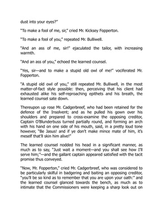
Analysis: We may want to examine how noise, or uncertain source terms,
affect the system. Consider, for example, a wind turbine (Figure 1.1). The
wind exerts a force on the turbine, and the strength of this force fluctuates
unpredictably. We may model these fluctuations as noise, and ask how they
cause the construction to vibrate. To answer this question, we must have a
model of how the noise enters the system, i.e., g, as well as how the system
dynamics respond, i.e., f. Figure 1.1 shows a simulation from a model with
three state variables, i.e., Xt is a 3-vector containing force on the turbine
and the position and velocity of the hub. The figure compares a stochastic
simulation with a noise-free simulation. Based on such a simulation, or a
mathematical analysis of the model, we can get statistics of force, position
and velocity. These statistics are important to assess the wear and tear on
the turbine, and also affect the regularity of the electrical power which is
generated by the turbine.
Time series analysis: We may have a time series of measurements taken
from the system. Based on these measurements, we may want to estimate
DOI: 10.1201/9781003277569-1 1
21.
2 StochasticDifferential Equations for Science and Engineering
q
0
m
k
c
F
)RUFH
í
3RVLWLRQ
í
7LPH
9HORFLW
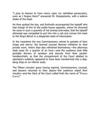
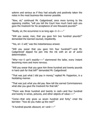
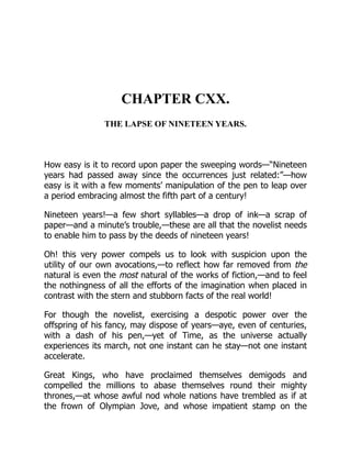
Figure 1.1 A wind turbine is affected by fluctuations in wind speed which
causes it to oscillate. We model the fluctuations as low-pass filtered noise
and the response of the construction as a linear mass-spring-damper sys-
tem. Solid lines: Simulated force, position and velocity from a stochastic
simulation of a dimensionless model. Dashed lines: Noise-free simula-
tion. The details of this model are given in Exercise 5.5. Photo credit:
CC BY-SA 4.0.
parameters in the differential equation, i.e., in f; we may want to know how
large loads the structure has been exposed to, and we may want to predict
the future production of electrical power. To answer these questions, we must
perform a statistical analysis on the time series. When we base time series
analysis on stochastic differential equations, we can use insight in the system
dynamics to fix the structure of f and maybe of g. The framework lets us
treat statistical errors correctly when estimating unknown parameters and
when assessing the accuracy with which we can estimate and predict.
Optimization and control: We may want to design a control system that
dampens the fluctuations that come from the wind. On the larger scale of the
electrical grid, we may want a control system to ensure that the power supply
meets the demand and so that voltages and frequencies are kept at the correct
values. To design such control systems optimally, we need to take into account
the nature of the disturbances that the control system should compensate for.
22.
Introduction 3
í
í
í
í
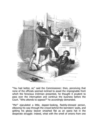
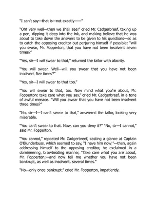
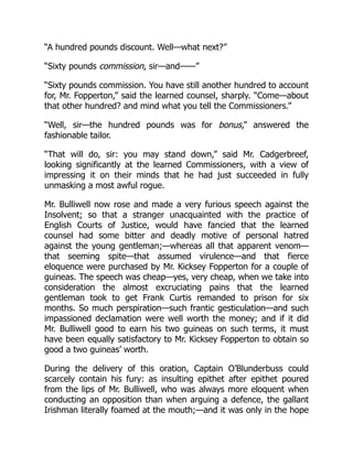
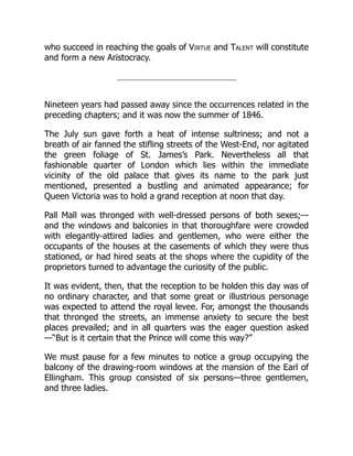
Figure 1.2 A small particle embedded in the two-dimensional flow around
a cylinder. The thin lines are streamlines, i.e., the paths a water molecule
follows, neglecting diffusion. The thick black line is a simulated random
trajectory of a particle, which is transported with the flow, but at the
same time subjected to molecular diffusion.
Motion of a Particle Embedded in a Fluid Flow
Let us examine in some more detail the origin and form of the noise term
ξt in (1.1). Figure 1.2 displays water flowing in two dimensions around a
cylinder.1
In absence of diffusion, water molecules will follow the streamlines.
A small particle will largely follow the same streamlines, but is also subject
to diffusion, i.e., random collisions with neighboring molecules which cause it
to deviate from the streamlines. Collisions are frequent but each cause only a
small displacement, so the resulting path is erratic.
In absence of diffusion, we can find the trajectory of the particle by solving
the ordinary differential equation
dXt
dt
= f(Xt).
Here, Xt ∈ R2
is the position in the plane of the particle at time t. The
function f(·) is the flow field, so that f(x) is a vector in the plane indicating
the speed and direction of the water flow at position x. To obtain a unique
solution, this equation needs an initial condition such as X0 = x0 where x0
is the known position at time 0. The trajectory {Xt : t ∈ R} is exactly a
streamline.
1The flow used here is irrotational, i.e., potential flow. Mathematically, this is convenient
even if physically, it may not be the most meaningful choice.
23.
4 StochasticDifferential Equations for Science and Engineering
To take the molecular diffusion into account, i.e., the seemingly random
motion of a particle due to collisions with fluid molecules, we add “white
noise” ξt to the equation
dXt
dt
= f(Xt) + g ξt. (1.2)
Here, g is the (constant) noise intensity, and ξt is a two-vector. The trajec-
tory in Figure 1.2 has been simulated as follows: We discretize time. At each
time step, we first advect the particle in the direction of a streamline, then we
shift it randomly by adding a perturbation which is sampled from a bivariate
Gaussian where each component has mean 0 and variance g2
h. Specifically,
Xt+h = Xt + f(Xt) h + g ξ
(h)
t where ξ
(h)
t ∼ N(0, hI).
Here, h is the time step and the superscript in ξ
(h)
t indicates that the noise term
depends on the time step, while I is a 2-by-2 identity matrix. If we let the par-
ticle start at a fixed position X0, the resulting positions {Xh, X2h, X3h, . . .}
will each be a random variable, so together they constitute a stochastic pro-
cess. This algorithm does not resolve the position between time steps; when
we plot the trajectory, we interpolate linearly.
We hope that the position Xt at a given time t will not depend too much
on the time step h as long as h is small enough. This turns out to be the case,
if we choose the noise term in a specific way, viz.
ξ
(h)
t = Bt+h − Bt,
where {Bt} is a particular stochastic process, namely Brownian motion. Thus,
we should start by simulating the Brownian motion, and next compute the
noise terms ξ
(h)
t from the Brownian motion; we will detail exactly how to
do this later. Brownian motion is key in the theory of stochastic differential
equations for two reasons: First, it solves the simplest stochastic differential
equation, dXt/dt = ξt, and second, we use it to represent the noise term in any
stochastic differential equation. With this choice of noise ξ
(h)
t , we can rewrite
the recursion with the shorthand
ΔXt = f(Xt) Δt + g ΔBt (1.3)
and since this turns out to converge as the time step h = Δt goes to zero, we
use the notation
dXt = f(Xt) dt + g dBt (1.4)
for the limit. This is our preferred notation for a stochastic differential equa-
tion. In turn, (1.3) is an Euler-type numerical method for the differential
equation (1.4), known as the Euler-Maruyama method.
If the particle starts at a given position X0 = x0, its position at a later time
t will be random, and we would like to know the probability density of the
24.
Introduction 5
positionφ(x, t). It turns out that this probability density φ(x, t) is governed
by a partial differential equation of advection-diffusion type, viz.
∂φ
∂t
= −∇ · (fφ −
1
2
g2
∇φ)
with appropriate boundary conditions. This is the same equation that governs
the concentration of particles, if a large number of particles is released and
move independently of each other. This equation is at the core of the theory of
transport by advection and diffusion, and now also a key result in the theory
of stochastic differential equations.
We can also ask, what is the probability that the particle hits the cylinder,
depending on its initial position. This is governed by a related (specifically,
adjoint) partial differential equation.
There is a deep and rich connection between stochastic differential equa-
tions and partial differential equations involving diffusion terms. This connec-
tion explains why we, in general, use the term diffusion processes for solutions
to stochastic differential equations. From a practical point of view, we can ana-
lyze PDE’s by simulating SDE’s, or we can learn about the behavior of specific
diffusion processes by solving associated PDE’s analytically or numerically.
Population Growth and State-Dependent Noise
In the two previous examples, the wind turbine and the dispersing molecule,
the noise intensity g(x) in (1.1) was a constant function of the state x. If
all models had that feature, this book would be considerably shorter; some
intricacies of the theory only arise when the noise intensity is state-dependent.
State-dependent noise intensities arise naturally in population biology, for
example. A model for the growth of an isolated bacterial colony could be:
dXt = rXt(1 − Xt/K) dt + g(Xt) dBt. (1.5)
Here, r 0 is the specific growth rate at low abundance, while K 0 is the
carrying capacity. Without noise, i.e., with g(x) ≡ 0, this is the logistic growth
model; see Figure 1.3. Dynamics of biological systems is notoriously noisy, so
we have included a noise term g(Xt) dBt and obtained a stochastic logistic
growth model. Here, it is critical that the noise intensity g(x) depends on the
abundance x; otherwise, we can get negative abundances Xt! To avoid this,
we must require that the noise intensity g(x) vanishes at the origin, g(0) = 0,
so that a dead colony stays dead. Figure 1.3 includes two realizations of the
solution {Xt} with the choice g(x) = σx. For this situation, the theory allows
us to answer the following questions:
1. How is the state Xt distributed, in particular as time t → ∞? Again,
we can pose partial differential equations of advection-diffusion type to
answer this, and the steady-state distribution can be found in closed
form. For example, we can determine the mean and variance.
25.
6 StochasticDifferential Equations for Science and Engineering
W
;
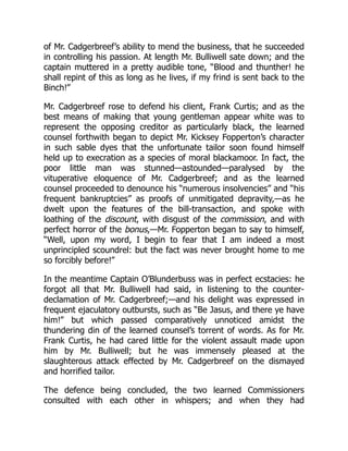
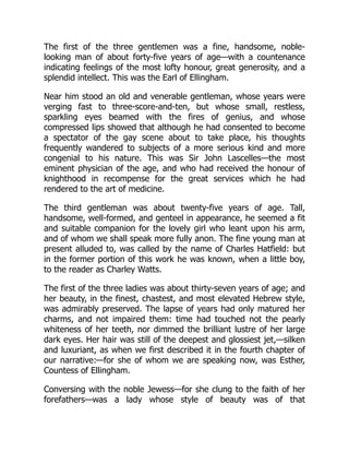
Figure 1.3 Two simulated sample paths (solid and dotted erratic curves)
of the stochastic logistic growth model (1.5) with g(x) = σx of a bac-
terial population. A noise-free simulation is included (thin black line).
Parameters are r = K = 1, σ = 0.1, X0 = 0.01. The computational time
step used is 0.001.
2. What is the temporal pattern of fluctuations in {Xt}? We shall see
that {Xt} is a Markov process, which allows us to characterize these
fluctuations. We can assess their time scale through their stochastic
Lyapunov exponent, which for this example leads to a time scale of
1/(r − σ2
/2), when the noise is weak and the process is in stochastic
steady state.
3. Does a small colony risk extinction? For this particular model with these
particular parameters, it turns out that the answer is “no”. With other
parameters, the answer is that the colony is doomed to extinction, and
for other noise structures, the answer is that there is a certain probability
of extinction, which depends on the initial size of the colony. These
questions are answered by stochastic stability theory as well as by the
theory of boundary behavior and classification.
However, before we can reach these conclusions, we must consider the
equation (1.5) carefully. We call it a stochastic differential equation, but it
should be clear from Figure 1.3 that the solutions are nowhere differentiable
functions of time. This means that we should not take results from standard
calculus for granted. Rather, we must develop a stochastic calculus which
applies to diffusion processes. In doing so, we follow in the footsteps of Kiyosi
Itô, who took as starting point an integral version of the equation (1.5), in
order to circumvent the problem that stochastic differential equations have
26.
Introduction 7
non-differentiablesolutions. The resulting Itô calculus differs from standard
calculus, most notably in its chain rule, which includes second order terms.
Overview of the Book
This book is in three parts. The core is Itô’s stochastic calculus in part 2: It
describes stochastic integrals, stochastic calculus, stochastic differential equa-
tions, and the Markov characterization of their solutions.
Before embarking on this construction, part 1 builds the basis. We first
consider molecular diffusion as a transport processes (Chapter 2); this gives
a physical reference for the mathematics. We then give a quick introduction
to measure-theoretic probability (Chapter 3) after which we study Brown-
ian motion as a stochastic process (Chapter 4). Chapter 5 concerns the very
tractable special case of linear systems such as the wind turbine (Figure 1.1).
At this point we are ready for the Itô calculus in part 2.
Finally, part 3 contains four chapters which each gives an introduction
to an area of application. This concerns estimation and time series analysis
(Chapter 10), quantifying expectations to the future (Chapter 11), stability
theory (Chapter 12) and finally optimal control (Chapter 13).
Exercises, Solutions, and Software
In science and engineering, what justifies mathematical theory is that it lets us
explain existing real-world systems and build new ones. The understanding
of mathematical constructions must go hand in hand with problem-solving
and computational skills. Therefore, this book contains exercises of differ-
ent kinds: Some fill in gaps in the theory and rehearse the ability to ar-
gue mathematically. Others contain pen-and-paper exercises while yet oth-
ers require numerical analysis on a computer. Solutions are provided at
https://github.com/Uffe-H-Thygesen/SDEbook. There, also code which re-
produces all figures is available. The computations use a toolbox, SDEtools for
R, which is available at https://github.com/Uffe-H-Thygesen/SDEtools.
There is no doubt that stochastic differential equations are becoming more
widely applied in many fields of science and engineering, and this by itself jus-
tifies their study. From a modeler’s perspective, it is attractive that our un-
derstanding of processes and dynamics can be summarized in the drift term
f in (1.1), while the noise term ξt (or Bt) manifests that our models are
always incomplete descriptions of actual systems. The mathematical theory
ties together several branches of mathematics – ordinary and partial differen-
tial equations, measure and probability, statistics, and optimization. As you
develop an intuition for stochastic differential equations, you will establish
27.
8 StochasticDifferential Equations for Science and Engineering
interesting links between subjects that may at first seem unrelated, such as
physical transport processes and propagation of noise. I have found it im-
mensely rewarding to study these equations and their solutions. My hope is
that you will, too.
C H AP T E R 2
Diffusive Transport and
Random Walks
The theory of stochastic differential equations uses a fair amount of mathe-
matical abstraction. If you are interested in applying the theory to science and
technology, it may make the theory more accessible to first consider a phys-
ical phenomenon, which the theory aims to describe. One such phenomenon
is molecular diffusion, which was historically a key motivation for the theory
of stochastic differential equations.
Molecular diffusion is a transport process in fluids like air and water and
even in solids. It is caused by the erratic and unpredictable motion of molecules
which collide with other molecules. The phenomenon can be viewed at a
microscale, where we follow the individual molecule, or at a macroscale, where
it moves material from regions with high concentration to regions with low
concentration (Figure 2.1).
The macroscale description of diffusion involves the concentration C =
C(x, t) of a substance and how it evolves in time. Here, x is the spatial position
while t is the time; the concentration measures how many molecules there are
in a given region. In this chapter, we derive and analyze the advection-diffusion
equation which governs the concentration:
∂C
∂t
= −∇ · (uC − D∇C).
In contrast, the microscale description of diffusion is that each single molecule
moves according to a stochastic process, which is governed by a stochastic
differential equation. It turns out that we can use the advection-diffusion
equation to compute the statistics of this process. In turn, we can simulate
the random motion of the molecule, which leads to Monte Carlo methods for
analyzing the advection-diffusion equation. That is, there is a precise coupling
between the microscale and the macroscale, between stochastic differential
equations and partial differential equations.
DOI: 10.1201/9781003277569-2 11
31.
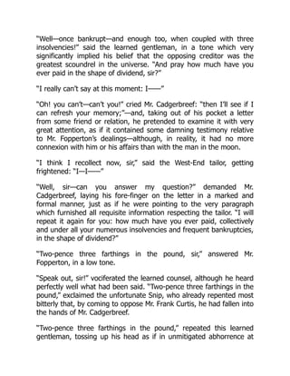
12 StochasticDifferential Equations for Science and Engineering
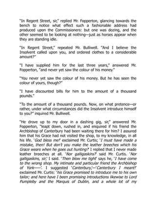
Figure 2.1 Diffusion in a container in two dimensions. Top panels: Con-
centration fields. Bottom panels: Position of 100 molecules. Left panels:
Initially, the solute is concentrated at the center. Right panels: After
some time, the solute is less concentrated. The bottom right panel also
includes the trajectory of one molecule; notice its irregular appearance.
2.1 DIFFUSIVE TRANSPORT
In this section, we model how a substance spreads in space due to molecular
diffusion. Think of smoke in still air, or dye in still water. The substance is
distributed over a one-dimensional space R. Let μt([a, b]) denote the amount
of material present in the interval [a, b] at time t. Mathematically, this μt is
a measure. We may measure the substance in terms of number of molecules
or moles, or in terms of mass, but we choose to let μt be dimensionless. We
assume that μt admits a density, which is the concentration C(·, t) of the
substance, so that the amount of material present in any interval [a, b] can be
found as the integral of the concentration over the interval:
μt([a, b]) =
b
a
C(x, t) dx.
The density has unit per length; if the underlying space had been two or three
dimensional, then C would have unit per length squared or cubed, i.e., per
area or per volume. The objective of this section is to pose a partial differential
equation, the diffusion equation (2.3), which governs the time evolution of this
concentration C.
32.
Diffusive Transport andRandom Walks 13
C
x
a b
μ
Ja
Jb
Figure 2.2 Conservation in one dimension. The total mass in the interval
[a, b] is μt([a, b]) =
b
a C(x, t) dx, corresponding to the area of the shaded
region. The net flow into the interval [a, b] is J(a) − J(b).
2.1.1 The Conservation Equation
We first establish the conservation equation
∂C
∂t
+
∂J
∂x
= 0, (2.1)
which expresses that mass is redistributed in space by continuous movements,
but neither created, lost, nor teleported instantaneously between separated
regions in space. To see that this equation holds, note that transport may
then be quantified with a flux J(x, t), which is the net amount of material
that crosses the point x per unit time, from left to right. The flux has physical
dimension “per time”. Then, the amount of material in the interval [a, b] is
only changed by the net influx at the two endpoints, i.e.,
d
dt
μt([a, b]) = J(a, t) − J(b, t).
See Figure 2.2. Assume that the flux J is differentiable in x, then
J(a, t) − J(b, t) = −
b
a
∂J
∂x
(x, t) dx.
On the other hand, since μt is given as an integral, we can use the Leibniz
integral rule to find the rate of change by differentiating under the integral
sign:
d
dt
μt([a, b]) =
b
a
∂C
∂t
(x, t) dx.
Here, we assume that C is smooth so that the Leibniz integral rule applies.
Combining these two expressions for the rate of change of material in [a, b],
we obtain: b
a
∂C
∂t
(x, t) +
∂J
∂x
(x, t)
dx = 0.
33.
14 StochasticDifferential Equations for Science and Engineering
Since the interval [a, b] is arbitrary, we can conclude that the integrand is
identically 0, or
∂C
∂t
(x, t) +
∂J
∂x
(x, t) = 0.
This is known as the conservation equation. To obtain a more compact nota-
tion, we often omit the arguments (x, t), and we use a dot (as in Ċ) for time
derivative and a prime (as in J
) for spatial derivative. Thus, we can state the
conservation equation compactly as
Ċ + J
= 0.
2.1.2 Fick’s Laws
Fick’s first law for diffusion states that the diffusive flux is proportional to the
concentration gradient:
J(x, t) = −D
∂C
∂x
(x, t) or simply J = −DC
. (2.2)
This means that the diffusion will move matter from regions of high concen-
tration to regions of low concentration. The constant of proportionality, D,
is termed the diffusivity and has dimensions area per time (also when the
underlying space has more than one dimension). The diffusivity depends on
the diffusing substance, the background material it is diffusing in, and the
temperature. See Table 2.1 for examples of diffusivities.
Fick’s first law (2.2) is empirical but consistent with a microscopic model
of molecule motion, as we will soon see. Combining Fick’s first law with the
conservation equation (2.1) gives Fick’s second law, the diffusion equation:
Ċ = (DC
)
. (2.3)
This law predicts, for example, that the concentration will decrease at a peak,
i.e., where C
= 0 and C
0. In many physical situations, the diffusivity D
is constant in space. In this case, we may write Fick’s second law as
Ċ = DC
when D is constant in space, (2.4)
i.e., the rate of increase of concentration is proportional to the spatial curva-
ture of the concentration. However, constant diffusivity is a special situation,
and the general form of the diffusion equation is (2.3).
TABLE 2.1 Examples of Diffusivities
Process Diffusivity [m2
/s]
Smoke particle in air at room temperature 2 × 10⁻⁵
Salt ions in water at room temperature 1 × 10⁻⁹
Carbon atoms in iron at 1250 K 2 × 10⁻¹¹
34.
Diffusive Transport andRandom Walks 15
Biography: Adolph Eugen Fick (1829–1901)
A German pioneer in biophysics with a background
in mathematics, physics, and medicine. Interested
in transport in muscle tissue, he used the transport
of salt in water as a convenient model system. In
a sequence of papers around 1855, he reported on
experiments as well as a theoretical model of trans-
port, namely Fick’s laws, which were derived as an
analogy to the conduction of heat.
Exercise 2.1: For the situation in Figure 2.2, will the amount of material in
the interval [a, b] increase or decrease in time? Assume that (2.4) applies, i.e.,
the transport is diffusive and the diffusivity D is constant in space.
For the diffusion equation to admit a unique solution, we need an initial
condition C(x, 0) and spatial boundary conditions. Typical boundary condi-
tions either fix the concentration C at the boundary, i.e., Dirichlet conditions,
or the flux J. In the latter case, since the flux J = uC−D∇C involves both the
concentration C and its gradient ∇C, the resulting condition is of Robin type.
In many situations, the domain is unbounded so that the boundary condition
concerns the limit |x| → ∞.
2.1.3 Diffusive Spread of a Point Source
We now turn to an important situation where the diffusion equation admits
a simple solution in closed form: We take the spatial domain to be the entire
real line R, we consider a diffusivity D which is constant in space and time,
and we assume that the fluxes vanish in the limit |x| → ∞. Consider the initial
condition that one unit of material is located at position x0, i.e.,
C(x, 0) = δ(x − x0),
where δ is the Dirac delta. The solution is then a Gaussian bell curve:
C(x, t) =
1
√
2Dt
φ
x − x0
√
2Dt
. (2.5)
Here, φ(·) is the probability density function (p.d.f.) of a standard Gaussian
variable,
φ(x) =
1
√
2π
exp(−
1
2
x2
). (2.6)
Thus, the substance is distributed according to a Gaussian distribution with
mean x0 and standard deviation
√
2Dt; see Figure 2.3. This standard devia-
tion is a characteristic length scale of the concentration field which measures
35.
16 StochasticDifferential Equations for Science and Engineering
í í
3RVLWLRQP@
RQFHQWUDWLRQP@
7LPH V
7LPH V
7LPH V
Figure 2.3 Diffusive spread. The concentration field at times t = 1, 5, 10 s
with diffusivity D = 1 m2
/s and a unit amount of material, which ini-
tially is located at the point x = 0 m.
(half the) width of the plume; recall also that for a Gaussian, the standard
deviation is the distance from the mean to inflection point. We see that length
scales with the square root of time, or equivalently, time scales with length
squared (Figure 2.4). This scaling implies that molecular diffusion is often
to be considered a small-scale process: on longer time scales or larger spatial
scales, other phenomena may take over and be more important. We will return
to this point later, in Section 2.4.
Exercise 2.2: Insert solution (2.5) into the diffusion equation and verify that
it satisfies the equation. In which sense does the solution also satisfy the initial
condition?
7LPHW
/HQJWKVFDOH
'W
Figure 2.4 Square root relationship between time and diffusive length
scale.
36.
Diffusive Transport andRandom Walks 17
Exercise 2.3: Compute the diffusive length scale for smoke in air, and for
salt in water, for various time scales between 1 second and 1 day.
Solution (2.5) is a fundamental solution (or Green’s function) with which
we may construct also the solution for general initial conditions. To see this, let
H(x, x0, t) denote the solution C(x, t) corresponding to the initial condition
C(x, 0) = δ(x − x0), i.e., (2.5). Since the diffusion equation is linear, a linear
combination of initial conditions results in the same linear combination of
solutions. In particular, we may write a general initial condition as a linear
combination of Dirac deltas:
C(x, 0) =
+∞
−∞
C(x0, 0) · δ(x − x0) dx0.
We can then determine the response at time t from each of the deltas, and
integrate the responses up:
C(x, t) =
+∞
−∞
C(x0, 0) · H(x, x0, t) dx0. (2.7)
Note that here we did not use the specific form of the fundamental solution;
only linearity of the diffusion equation and existence of the fundamental so-
lution. In fact, this technique works also when diffusivity varies in space and
when advection is effective in addition to diffusion, as well as for a much larger
class of problems. However, when the diffusivity is constant in space, we get a
very explicit result, namely that the solution is the convolution of the initial
condition with the fundamental solution:
C(x, t) =
+∞
−∞
1
(4πDt)1/2
exp
−
1
2
|x − x0|2
2Dt
C(x0, 0) dx0.
2.1.4 Diffusive Attenuation of Waves
Another important situation which admits solutions in closed form is the
diffusion equation (2.4) with the initial condition
C(x, 0) = sin kx,
where k is a wave number, related to the wavelength L by the formula kL = 2π.
In this case, the solution is
C(x, t) = exp(−λt) sin kx with λ = Dk2
. (2.8)
Exercise 2.4: Verify this solution.
Thus, harmonic waves are eigenfunctions of the diffusion operator; that
is, they are attenuated exponentially while preserving their shape. Note that
the decay rate λ (i.e., minus the eigenvalue) is quadratic in the wave number
37.
18 StochasticDifferential Equations for Science and Engineering
k. Another way of expressing the same scaling is that the half-time of the
attenuation is
T1/2 =
1
λ
log 2 =
log 2
4π2
L2
D
,
i.e., the half time is quadratic in the wave length: Twice as long waves persist
four times longer. See Figure 2.5. We recognize the square root/quadratic
relationship between temporal and spatial scales from Figure 2.4.
Recall that we used the fundamental solution (2.5) to obtain the response
of a general initial condition. We can do similarly with the harmonic solution
(2.8), although we need to add the cosines or, more conveniently, use complex
exponentials. Specifically, if the initial condition is square integrable, then it
can be decomposed into harmonics as
C(x, 0) =
1
2π
+∞
−∞
C̃(k, 0) eikx
dk,
where C̃(k, 0) is the (spatial) Fourier transform
C̃(k, 0) =
+∞
−∞
C(x, 0) e−ikx
dx.
Note that different authors use slightly different definitions of the Fourier
transform. Now, each wave component exp(ikx) is attenuated to exp(−Dk2
t+
ikx), so the Fourier transform of C(x, t) is
C̃(k, t) = C̃(k, 0) e−Dk2
t
.
í
í
[
í
í
[
Figure 2.5 Attenuation of spatial waves by diffusion. Here the diffusivity
is D = 1 and the terminal time is T = 0.01. Solid lines: At time 0, the
amplitude is 1. Dashed lines: At time T, the wave is attenuated – how
much depends on the wave number. Left panel: A long wave is attenuated
slowly. Right panel: A shorter wave is attenuated more quickly.
38.
Diffusive Transport andRandom Walks 19
We can now find the solution C(x, t) by the inverse Fourier transform:
C(x, t) =
1
2π
+∞
−∞
C̃(k, 0) e−Dk2
t+ikx
dk.
One interpretation of this result is that short-wave fluctuations (large |k|)
in the initial condition are smoothed out rapidly while long-wave fluctuations
(small |k|) persist longer; the solution is increasingly dominated by longer and
longer waves which decay slowly as the short waves disappear.
2.2 ADVECTIVE AND DIFFUSIVE TRANSPORT
In many physical situations, diffusion is not the sole transport mechanism: A
particle with higher density than the surrounding fluid will have a movement
with a downwards bias. If the fluid is flowing, then the particle will have a
tendency to follow the flow (Figure 2.6). These situations both amount to a
directional bias in the movement, so we focus on the latter.
Let the flow field be u(x, t). If we use Xt to denote the position of a fluid
element at time t, then Xt satisfies the differential equation
d
dt
Xt = u(Xt, t).
Consider again a solute which is present in the fluid, and as before let C(x, t)
denote the concentration of the solute at position x and time t. If the material
is a perfectly passive tracer (i.e., material is conserved and transported with
the bulk motion of the fluid), then the flux of material is the advective flux:
JA(x, t) = u(x, t) C(x, t).
[
[
[7
Figure 2.6 A fluid flow in one dimension which transports a substance.
The plume is advected to the right with the flow; at the same time it
diffuses out. The diffusivity is D = 1, the advection is u = 2.5, and the
terminal time is T = 4.
39.
20 StochasticDifferential Equations for Science and Engineering
If in addition molecular diffusion is in effect, then according to Fick’s first law
(2.2) this gives rise to a diffusive flux JD = −DC
. We may assume that these
two transport mechanisms operate independently, so that the total flux is the
sum of the advective and diffusive fluxes:
J(x, t) = u(x, t) C(x, t) − D(x)
∂C
∂x
(x, t),
or simply J = uC − DC
. Inserting this into the conservation equation (2.1),
we obtain the advection-diffusion equation for the concentration field:
Ċ = −(uC − DC
)
. (2.9)
A simple case is when u and D are constant, the initial condition is a Dirac
delta, C(x, 0) = δ(x − x0), where x0 is a parameter, and the flux vanishes as
|x| → ∞. Then the solution is:
C(x, t) =
1
√
4πDt
exp
−
(x − ut − x0)2
4Dt
, (2.10)
which is the probability density function of a Gaussian random variable with
mean x0 + ut and variance 2Dt. Advection shifts the mean with constant
rate, as if there had been no diffusion, and diffusion gives rise to a linearly
growing variance while preserving the Gaussian shape, as in the case of pure
diffusion (i.e., diffusion without advection). This solution is important, but
also a very special case: In general, when the flow is not constant, it will affect
the variance, and the diffusion will affect the mean.
Exercise 2.5:
1. Verify the solution (2.10).
2. Solve the advection-diffusion equation (2.9) on the real line with con-
stant u and D with the initial condition C(x, 0) = sin(kx) or, if you
prefer, C(x, 0) = exp(ikx).
2.3 DIFFUSION IN MORE THAN ONE DIMENSION
Consider again the one-dimensional situation in Figure 2.2. In n dimensions,
the interval [a, b] is replaced by a region V ⊂ Rn
. Let μt(V ) denote the amount
of the substance present in this region. This measure can be written in terms
of a volume integral of the density C:
μt(V ) =
V
C(x, t) dx.
Here x = (x1, . . . , xn) ∈ Rn
and dx is the volume of an infinitesimal volume
element. The concentration C has physical dimension “per volume”, i.e., SI
40.
Diffusive Transport andRandom Walks 21
unit m−n
, since μt(V ) should still be dimensionless. The flux J(x, t) is a vector
field, i.e., a vector-valued function of space and time; in terms of coordinates,
we have J = (J1, . . . , Jn). The defining property of the flux J is that the net
rate of exchange of matter through a surface ∂V is
∂V
J(x, t) · ds(x).
Here, ds is the surface element at x ∈ ∂V , a vector normal to the surface. The
flux J has SI unit m−n+1
s−1
. Conservation of mass now means that the rate
of change in the amount of matter present inside V is exactly balanced by the
rate of transport over the boundary ∂V :
V
Ċ(x, t) dx +
∂V
J(x, t) · ds(x) = 0, (2.11)
where ds is directed outward. This balance equation compares a volume inte-
gral with a surface integral. We convert the surface integral to another volume
integral, using the divergence theorem (the Gauss theorem), which equals the
flow out of the control volume with the integrated divergence. Specifically,
V
∇ · J dx =
∂V
J · ds.
In terms of coordinates, the divergence is ∇ · J = ∂J1/∂x1 + · · · + ∂Jn/∂xn.
Substituting the surface integral in (2.11) with a volume integral, we obtain
V
Ċ(x, t) + ∇ · J(x, t) dx = 0.
Since the control volume V is arbitrary, we get
Ċ + ∇ · J = 0, (2.12)
which is the conservation equation in n dimensions, in differential form.
Fick’s first law in n dimensions relates the diffusive flux to the gradient of
the concentration field:
J = −D∇C,
where the gradient ∇C has coordinates (∂C/∂x1, . . . , ∂C/∂xn). Often, the
diffusivity D is a scalar material constant, so that the relationship between
concentration gradient and diffusive flux is invariant under rotations. We then
say that the diffusion is isotropic. However, in general D is a matrix (or a ten-
sor, if we do not make explicit reference to the underlying coordinate system).
Then, the diffusive flux is not necessarily parallel to the gradient, and its
strength depends on the direction of the gradient. These situations can arise
when the diffusion takes place in an anisotropic material, or when the dif-
fusion is not molecular but caused by other mechanisms such as turbulence.
Anisotropic diffusion is also the standard situation when the diffusion model
does not describe transport in a physical space, but rather stochastic dynamics
in a general state space of a dynamic system.
41.
22 StochasticDifferential Equations for Science and Engineering
Fick’s second law can now be written as
Ċ = ∇ · (D∇C).
When the diffusivity is constant and isotropic, this reduces to Ċ = D∇2
C.
Here ∇2
is the Laplacian ∇2
= ∂2
∂x2
1
+ · · · + ∂2
∂x2
n
, a measure of curvature.
To take advection into account, we assume a flow field u with coordinates
(u1, . . . , un). The advective flux is now uC and the advection-diffusion equa-
tion is
Ċ = −∇ · (uC − D∇C). (2.13)
2.4 RELATIVE IMPORTANCE OF ADVECTION AND DIFFUSION
We have now introduced two transport processes, advection and diffusion,
which may be in effect simultaneously. It is useful to assess the relative im-
portance of the two.
Consider the solution (2.10) corresponding to constant advection u, con-
stant diffusion D, and the initial condition C(x, 0) = δ(x − xo). At time t, the
advection has moved the center of the plume a distance |u|t, while the diffu-
sive length scale – the half width of the plume – is
√
2Dt. These length scales
are shown in Figure 2.7 as functions of the time scale. Notice that initially,
when time t is sufficiently small, the diffusive length scale is larger than the
advective length scale, while for sufficiently large time t the advective length
scale dominates. This justifies our earlier claim that diffusion is most powerful
at small scales. The two length scales are equal when
t =
2D
u2
.
In stead of fixing time and computing associated length scales, one may fix
a certain length scale L and ask about the corresponding time scales associated
with advective and diffusive transport: The advective time scale is L/u while
7LPHW
/HQJWKVFDOHV
'LIIXVLYH
$GYHFWLYH
Figure 2.7 Advective (dashed) and diffusive (solid) length scale as func-
tion of time scale for the dimensionless model with u = D = 1.
42.
Diffusive Transport andRandom Walks 23
the diffusive time scale is L2
/2D. We define the Péclet number as the ratio
between the two:
Pe = 2
Diffusive time scale
Advective time scale
=
Lu
D
.
It is common to include factor 2 in order to obtain a simpler final expression,
but note that different authors may include different factors. Regardless of the
precise numerical value, a large Péclet number means that the diffusive time
scale is larger than the advective time scale. In this situation, advection is a
more effective transport mechanism than diffusion at the given length scale;
that is, the transport is dominated by advection. Conversely, if the Péclet
number is near 0, diffusion is more effective than advection at the given length
scale. Such considerations may suggest to simplify the model by omitting the
least significant term, and when done cautiously, this can be a good idea.
The analysis in this section has assumed that u and D were constant.
When this is not the case, it is customary to use “typical” values of u and D
to compute the Péclet number. This can be seen as a useful heuristic, but can
also be justified by the non-dimensional versions of the transport equations,
where the Péclet number enters. Of course, exactly which “typical values”
are used for u and D can be a matter of debate, but this debate most often
affects digits and not orders of magnitude. Even the order of magnitude of the
Péclet number is a useful indicator if the transport phenomenon under study
is dominated by diffusion or advection.
Example 2.4.1 Consider the advection-diffusion equation (2.13) in two di-
mensions, where the flow u(x) is around a cylinder. We non-dimensionalize
space so that the cylinder is centered at the origin and has radius 1, and non-
dimensionalize time so that the flow velocity far from the cylinder is 1. Then,
the flow is, in polar coordinates (r, θ) with x = r cos θ, y = r sin θ,
ur(r, θ) = (1 − r−2
) cos θ, uθ = −(1 + r−2
) sin θ.
This is called irrotational flow in fluid mechanics (Batchelor, 1967). A unit of
material is released at time t = 0 at position x = −3, y = −0.5. We solve the
advection-diffusion equation for t ∈ [0, 2.5] for three values of the diffusivity
D: D = 1, D = 0.1, and D = 0.01, leading to the three Péclet numbers 1, 10,
and 100. Figure 2.8 shows the solution at time t = 2.5 for the three Péclet
numbers. Notice how higher Péclet numbers (lower diffusivity D) imply a more
narrow distribution of the material.
2.5 THE MOTION OF A SINGLE MOLECULE
We can accept Fick’s first equation as an empirical fact, but we would like
to connect it to our microscopic understanding. In this section, we present a
caricature of a microscopic mechanism which can explain Fickian diffusion:
Each individual molecule moves in an erratic and unpredictable fashion, due
43.
24 StochasticDifferential Equations for Science and Engineering
4 2 0 2 4
4
2
0
2
4
4 2 0 2 4
4
2
0
2
4
4 2 0 2 4
4
2
0
2
4
Figure 2.8 Concentrations C(x, t = 2.5) from Example 2.4.1, for flow
around a cylinder with diffusivities leading to different Péclet numbers.
Left panel: Pe = 1. Center panel: Pe = 10. Right panel: Pe = 100. In each
panel, the grayscale represents concentration relative to the maximum
concentration.
í
7LPHQV@
3RVLWLRQμP@
í
í
7LPHQV@
3RVLWLRQμP@
Figure 2.9 A random walk model of molecular motion. Left: A close-up
where individual transitions are visible. Right: A zoom-out where the
process is indistinguishable from Brownian motion.
to the exceedingly large number of collisions with other molecules, so that
only a probabilistic description of its trajectory is feasible. This phenomenon
is called Brownian motion.
Let Xt ∈ R denote the position at time t of a molecule, e.g., smoke in air,
still considering one dimension only. At regularly spaced points of time, a time
step h apart, the molecule is hit by an air molecule which causes a displacement
±k. This happens independently of what has happened previously (Figure
2.9).1
1Physcially, collisions cause changes in velocity rather than position, but the simple
picture is more useful at this point. We can argue that the velocity decays to 0 due to
viscous friction and that the molecule drifts a certain distance during this decay. The simple
model was used by Einstein (1905); extensions that take the velocity process into account
were the Langevin (1908) equation and the Ornstein-Uhlenbeck process (Uhlenbeck and
Ornstein, 1930) (Section 5.10).
44.
Diffusive Transport andRandom Walks 25
Biography: Robert Brown (1773–1858)
A Scottish botanist who in 1827 studied pollen im-
mersed in water under a microscope and observed
an erratic motion of the grains. Unexplained at
the time, we now attribute the motion to seem-
ingly random collision between the pollen and wa-
ter molecules. The physical phenomenon and its
mathematical model are named Brownian motion,
although many other experimentalists and theoreti-
cians contributed to our modern understanding of
the phenomenon.
In summary, the position {Xt : t ≥ 0} is a random walk:
Xt+h =
⎧
⎨
⎩
Xt + k w.p. (with probability) p,
Xt w.p. 1 − 2p,
Xt − k w.p. p.
.
Here, p ∈ (0, 1
2 ] is a parameter. The displacement in one time step, Xt+h −Xt,
has mean 0 and variance 2k2
p. Displacements over different time steps are
independent, so the central limit theorem applies. After many time steps, the
probability distribution of the displacement Xnh will be well approximated
by a Gaussian with mean 0 and variance 2k2
pn:
Xnh ∼ N(0, 2k2
pn). (2.14)
That is, Xnh will (approximately) have the probability density function
1
2k2pn
· φ(x/ 2k2pn),
where φ is still the p.d.f. of a standard Gaussian variable from (2.6). Next,
assume that we release a large number N of molecules at the origin, and that
they move independently. According to the law of large numbers, the number
of molecules present between x1 and x2 at time nh will be approximately
N
x2
x1
1
2k2pn
· φ(x/ 2k2pn) dx.
Notice that this agrees with equation (2.5), assuming that we take N = 1,
D = k2
p/h and t = nh.
We see that our cartoon model of molecular motion is consistent with the
results of the diffusion equation, if we assume that
45.
26 StochasticDifferential Equations for Science and Engineering
Biography: Albert Einstein (1879–1955)
In his Annus Mirabilis, Einstein (1905) published
not just on the photoelectric effect and on special
relativity, but also on Brownian motion as the result
of molecular collisions. His work connected pressure
and temperature with the motion of molecules, gave
credibility to statistical mechanics, and estimated
the size of atoms. Soon confirmed in experiments
by Jean Perrin, this work ended the debate whether
atoms really exist.
1. molecules take many small jumps, i.e., h and k are small, so that the
Central Limit Theorem is applicable at any length and time scale that
our measuring devices can resolve, and
2. there is a large number of molecules present and they behave indepen-
dently, so that we can ignore that their number will necessarily be inte-
ger, and ignore its variance.
Both of these assumptions are reasonable in many everyday situations
where molecular systems are observed on a macroscale, for example, when
breathing or making coffee.
To simulate the motion of a single molecule, if we only care about the
displacements after many collisions, we may apply the approximation (2.14)
recursively to get
Xt − Xs ∼ N(0, 2D(t − s)), when t s.
Here we have assumed that the steps in time and space are consistent with
the diffusivity, i.e., D = k2
p/h. This process {Xt} with independent and
stationary Gaussian increments is called (mathematical) Brownian motion.
Note that, physically, these properties should only hold when the time lag t−s
is large compared to the time h between molecular collisions, so mathematical
Brownian motion is only an appropriate model of physical Brownian motion
at coarse scale, i.e., for large time lags t − s. Mathematical Brownian motion
is a fundamental process. It is simple enough that many questions regarding
its properties can be given explicit and interesting answers, and we shall see
several of these later, in Chapter 4.
In many situations, we choose to work with standard Brownian motion,
where we take 2D = 1 so that the displacement Bt+h − Bt has variance equal
to the time step h. When time has the physical unit of seconds s, notice that
this means that Bt has the physical unit of
√
s!
46.
Diffusive Transport andRandom Walks 27
2.6 MONTE CARLO SIMULATION OF PARTICLE MOTION
The previous section considered diffusion only. To add advection, the mi-
croscale picture is that each particle is advected with the fluid while subject
to random collisions with other molecules which randomly perturb the parti-
cle. Thus, each particle performs a biased random walk. When the diffusivity
D and the flow u are constant in space and time, the Gaussian solution (2.10)
to the advection-diffusion equation applies. Then, a random walk model that
is consistent with the advection-diffusion equation is to sample the increments
ΔX = Xt − Xs from a Gaussian distribution
ΔX ∼ N(u · (t − s), 2D(t − s)).
Now what if the flow u = u(x, t) varies in space and time? To simulate the
trajectory of a single particle, it seems to be a reasonable heuristic to divide
the time interval [0, T] into N subintervals
0 = t0, t1, . . . , tN = T.
We first sample X0 from the initial distribution C(·, 0). Then, we sample the
remaining trajectory recursively: At each sub-interval [ti, ti+1], we approxi-
mate the flow field with a constant, namely u(Xti
, ti). This gives us:
Xti+1 ∼ N(Xti + u(Xti ) · Δti, 2D · Δti), (2.15)
where Δti = ti+1 −ti. It seems plausible that, as the time step in this recursion
goes to 0, this approximation becomes more accurate so that the p.d.f. of Xt
will approach the solution C(·, t) to the advection-diffusion equation (2.9).
This turns out to be the case, although we are far from ready to prove it.
Example 2.6.1 (Flow past a cylinder revisited) Example 2.4.1 and Fig-
ure 2.8 present solutions of the advection-diffusion equation for the case where
the flow goes around a cylinder. In the introduction, Figure 1.2 (page 3) show
a trajectory of a single molecule in the same flow. This trajectory is simulated
with the recursion (2.15), using a Péclet number of 200.
The Monte Carlo method, we have just described simulates the motion of
single molecules, chosen randomly from the ensemble. Monte Carlo simulation
can be used to compute properties of the concentration C, but can also answer
questions that are not immediately formulated using partial differential equa-
tions; for example, concerning the time a molecule spends in a region. Monte
Carlo methods are appealing in situations where analytical solutions to the
partial differential equations are not available, and when numerical solutions
are cumbersome, e.g., due to irregular geometries. Monte Carlo methods can
also be useful when other processes than transport are active, for example,
when chemical reactions take place on or between the dispersing particles.
47.
28 StochasticDifferential Equations for Science and Engineering
2.7 CONCLUSION
Diffusion is a transport mechanism, the mathematical model of which involves
the concentration field and the flux. Fick’s laws tell us how to compute the flux
for a given concentration field, which in turn specifies the temporal evolution
of the concentration field. This is the classical approach to diffusion, in the
sense of 19th century physics.
A microscopic model of diffusion involves exceedingly many molecules
which each move erratically and unpredictably, due to collisions with other
molecules. This statistical mechanical image of molecular chaos is consistent
with the continuous fields of classical diffusion, but brings attention to the mo-
tion of a single molecule, which we model as a stochastic process, a so-called
diffusion process. The probability density function associated with a single
molecule is advected with the flow while diffusing out due to unpredictable
collisions, in the same way the overall concentration of molecules spreads.
We can simulate the trajectory of a diffusing molecule with a stochastic re-
cursion (Section 2.6). This provides a Monte Carlo particle tracking approach
to solving the diffusion equation, which is useful in science and engineer-
ing: In each time step, the molecule is advected with the flow field but per-
turbed randomly from the streamline, modeling intermolecular collisions. This
Monte Carlo method is particular useful in high-dimensional spaces or complex
geometries where numerical solution of partial differential equations is difficult
(and analytical solutions are unattainable).
Molecular diffusion is fascinating and relevant in its own right, but has even
greater applicability because it serves as a reference and an analogy to other
modes of dispersal; for example, of particles in turbulent flows, or of animals
which move unpredictably (Okubo and Levin, 2001). At an even greater level
of abstraction, a molecule moving randomly in physical space is a archetypal
example of a dynamic system moving randomly in a general state space. When
studying such general systems, the analogy to molecular diffusion provides not
just physical intuition, but also special solutions, formulas and even software.
With the Monte Carlo approach to diffusion, the trajectory of the diffus-
ing molecule is the focal point, while the classical focal points (concentrations,
fluxes, and the advection-diffusion equation that connect them) become sec-
ondary, derived objects. This is the path that we follow from now on. In the
chapters to come, we will depart from the physical notion of diffusion, in or-
der to develop the mathematical theory of these random paths. While going
through this construction, it is useful to have Figure 2.1 and the image of
a diffusing molecule in mind. If a certain piece of mathematical machinery
seems abstract, it may be enlightening to consider the question: How can this
help describe the trajectory of a diffusing molecule?
48.
Diffusive Transport andRandom Walks 29
Factbox: [The error function] The physics literature often prefers the “er-
ror function” to the standard Gaussian cumulative distribution function.
The error function is defined as
erf(x) =
2
√
π
x
0
e−s2
ds,
and the complementary error function is
erfc(x) = 1 − erf(x) =
2
√
π
∞
x
e−s2
ds.
These are related to the standard Gaussian distribution function Φ(x) by
erfc(x) = 2 − 2Φ(
√
2x), Φ(x) = 1 −
1
2
erfc(x/
√
2).
erf(x) = 2Φ(
√
2x) − 1, Φ(x) =
1
2
+
1
2
erf(x/
√
2).
2.8 EXERCISES
Exercise 2.6:
1. Solve the diffusion equation (2.4) on the real line with a “Heaviside step”
initial condition
C(x, 0) =
0 when x 0,
1 when x 0.
.
Use boundary conditions limx→+∞ C(x, t) = 1 and limx→−∞ C(x, t) =
0.
Hint: If you cannot guess the solution, use formula (2.7) and manipulate
the integral into a form that resembles the definition of the cumulative
distribution function.
2. Consider the diffusion equation (2.4) on the positive half-line x ≥ 0
with initial condition C(x, 0) = 0 and boundary conditions C(0, t) = 1,
C(∞, t) = 0.
Hint: Utilize the solution of the previous question, and the fact that in
that question, C(0, t) = 1/2 for all t 0.
Exercise 2.7: It is useful to have simple bounds on the tail probabilities in
the Gaussian distribution, such as (Karatzas and Shreve, 1997):
x
1 + x2
φ(x) ≤ 1 − Φ(x) ≤
1
x
φ(x).
49.
30 StochasticDifferential Equations for Science and Engineering
which hold for x ≥ 0. Here, as always, Φ(·) is the c.d.f. of a standard Gaussian
variable X ∼ N(0, 1), so that 1 − Φ(x) = P(X ≥ x) =
∞
x
φ(y) dy with φ(·)
being the density, φ(x) = 1
√
2π
e− 1
2 x2
. A useful consequence is
1 − Φ(x) = φ(x) · (x−1
+ O(x−3
)).
1. Plot the tail probability 1 − Φ(x) for 0 ≤ x ≤ 6. Include the upper and
lower bound. Repeat, in a semi-logarithmic plot.
2. Show that the bounds hold. Hint: Show that the bounds hold as x → ∞,
and that the differential version of the inequality holds for x ≥ 0 with
reversed inequality signs.
Exercise 2.8: Consider pure diffusion in n 1 dimensions with a scalar
diffusion D, and a point initial condition C(x, 0) = δ(x − x0), where x ∈ Rn
and δ is the Dirac delta in n dimensions. Show that each coordinate can be
treated separately, and thus, that the solution is a Gaussian in n dimensions
corresponding to the n coordinates being independent, i.e.,
C(x, t) =
n
i=1
1
√
2Dt
φ
ei(x − xo)
√
2Dt
=
1
(4πDt)n/2
exp
−
1
2
|x − x0|2
2Dt
,
where ei is the ith unit vector.
50.
C H AP T E R 3
Stochastic Experiments
and Probability Spaces
To build the theory of stochastic differential equations, we need precise prob-
abilistic arguments, and these require an axiomatic foundation of probability
theory. This foundation is measure-theoretic and the topic of this chapter.
In science and engineering, probability is typically taught elementary, i.e.,
without measure theory. This is good enough for many applications, but it
does not provide firm enough ground for more advanced topics like stochas-
tic differential equations. One symptom of this is the existence of paradoxes
in probability: Situations, or brain teasers, where different seemingly valid
arguments give different results. Another symptom is that many elementary
introductions to probability fail to give precise definitions, but in stead only
offer synonyms such as “a probability is a likelihood”.
The measure-theoretic approach to probability constructs a rigorous the-
ory by considering stochastic experiments and giving precise mathematical
definitions of the elements that make up such experiments: Sample spaces,
realizations, events, probabilities, random variables, and information. To gain
intuition, we consider simple experiments such as tossing coins or rolling dice,
but soon we see that the theory covers also more complex experiments such
as picking random functions.
At the end, we reach a construction which is consistent with the elementary
approach, but covers more general settings. Therefore, there is no need to “un-
learn” the elementary approach. The measure theoretic approach may seem
abstract, but it gives precise mathematical meaning to concepts that not many
people find intuitive. Once one has become familiar with the concepts, they
can even seem natural, even if they are still technically challenging. A final
argument in favor of the measure-theoretic approach is that the mathematical
literature on stochastic differential equations is written in the language of
measure theory, so the vocabulary is necessary for anyone working in this
field, even if one’s interest is applications rather than theory.
DOI: 10.1201/9781003277569-3 31
51.
32 StochasticDifferential Equations for Science and Engineering
Ω
A
ω
Figure 3.1 In a stochastic experiment, Chance picks an outcome ω from
the sample space Ω. An event A is a subset of Ω and occurs or is true if
ω ∈ A. For the outcome ω in the figure, the event A did not occur.
3.1 STOCHASTIC EXPERIMENTS
The most fundamental concept in probability theory is the stochastic experi-
ment. This is a mathematical model of real-world experiments such as rolling
a die and observing the number of eyes.
Mathematically, a stochastic experiment involves a set containing all possi-
ble outcomes: The sample space Ω. We let ω denote an element in Ω; we call ω
an outcome or a realization. For the die experiment, we set Ω = {1, 2, 3, 4, 5, 6}.
The stochastic experiment is that some mechanism, or the Goddess of Chance,
selects one particular outcome ω from the sample space Ω (Figure 3.1).
A few other examples:
Statistical models: Statistical methods for data analysis are justified by
postulating that the data has been produced by a stochastic experiment. For
example, we may weigh an object n times, obtaining measurements y1, . . . , yn,
and postulating yi = μ + ei. Here, μ is the (unknown) true weight of the
object and ei is the ith measurement error. We take the sample space to be
Ω = Rn
and identify the outcome ω ∈ Ω with the measurement errors, i.e.,
ω = (e1, . . . , en).
Monte Carlo simulation: In computer simulations of stochastic ex-
periments, we rely on a random number generator which, ideally, produces
an infinite series of independent and identically distributed numbers {Zi ∈
R : i ∈ N}. Hence, the sample space is the set of sequences of real numbers,
Ω = RN
. If we take into account that computers only produce pseudo-random
numbers, we may identify the realization ω with the seed of the random num-
ber generator; this allows to repeat the stochastic experiment, picking the
same realization ω.
Diffusion and Brownian motion: In Chapter 2, we considered the
experiment of releasing a large number of molecules; say, dye in water. A
stochastic experiment is to pick one random molecule and record how its po-
sition changes in time. A mathematical model of this, in one dimension, is
Brownian motion (Chapter 4), where the sample space is Ω = C(R̄+, R),
the set of continuous real-valued functions defined on [0, ∞). We identify the
52.
Stochastic Experiments andProbability Spaces 33
randomly chosen continuous function ω ∈ Ω with the trajectory of the
molecule {Bt : t ≥ 0}.
Once the sample space Ω is defined, we next need events. Events are state-
ments about the outcome, such as “The die showed an even number” or “the
molecule hits x = 1 before time t = 1”. Once the experiment has been per-
formed, the statement is either true or false. Mathematically, an event A is
a subset of Ω containing those outcomes for which the statement is true. For
example:
• For the die experiment, the statement “The die shows an even number”
is the event {2, 4, 6}.
• For the linear regression model, an event is a subset of Rn
. One example
is the event “all the measurement errors are positive”, corresponding to
Rn
+.
This brings us to probabilities: The point of the stochastic model is to as-
sign probabilities to each event. For the die-tossing experiment, if the die is
fair, then P({2, 4, 6}) = 1/2, for example. This probability can be interpreted
in different ways. The frequentist view is that if we toss the die repeatedly, we
will eventually observe that the die has shown 2, 4 or 6 in half the tosses. The
subjective Bayesian view is that we subjectively believe the event {2, 4, 6} to
be as probable as the alternative, {1, 3, 5}, and aims for consistency in such
subjective beliefs. From an applied and pragmatic point of view, in some sit-
uations the frequentist view is justified, while in others the Bayesian view is
more appropriate; even other interpretations exist. Fortunately, the mathe-
matical construction in the following applies regardless of the interpretation.
Now the vocabulary is in place – sample space, outcomes, events, prob-
abilities – we need to specify the mathematical properties of these objects.
First, which events do we consider? For the example of the die, it is simple:
Any subset of Ω is allowed, including the empty set and Ω itself. Moreover,
if the die is fair, the probability of an event depends only on the number of
elements in it, P(A) = |A|/|Ω|.
For the statistical model, we could start by trying to make an event out of
each and every subset A of Rn
. In an elementary course on probability and
statistics, we would maybe postulate a probability density function f(e) for
each measurement error and claim independence such that
P(A) =
A
f(e1) · · · f(en) de1 · · · den.
Unfortunately, it turns out that there are subsets A of Rn
that are so patho-
logical that this integral is not defined – even for n = 1 and regardless of
how regular f is. You can accept this as a curious mathematical fact, or you
can look up the “Vitali set” in (Billingsley, 1995) or on Wikipedia. We need
53.
34 StochasticDifferential Equations for Science and Engineering
to exclude such “non-measurable” subsets of Rn
: They do not correspond to
events.
In elementary probability and statistics, we tend to ignore non-measurable
subsets of Rn
, which have little relevance in applications. However, for more
complicated sample spaces Ω, which appear in the study of stochastic processes
and in particular stochastic differential equations, this difficulty cannot be
ignored: Not all subsets of the sample space can be events, and we often need
careful analysis to determined which ones are.
When not every set A ⊂ Ω can be an event, which ones should be? Some
events are required for the theory to be useful. For example, in the scalar
case Ω = R, we want intervals to correspond to events, so that the statement
ω ∈ [a, b] is an event for any a and b. Moreover, it is imperative that our
machinery of logic works: If A is an event, then the complementary set Ac
must also be an event, so that the statement “not A” is valid. Next, if also
B is an event, then the intersection A ∩ B must also be an event, so that the
statement “A and B” is valid. More generally, in stochastic processes we often
consider infinite sequences of events, for instance when analyzing convergence.
So if {Ai : i ∈ N} is a sequence of events, then the statement “for each integer
i, the statement Ai holds” should be valid. In terms of subsets of sample space
Ω, this means that A1 ∩ A2 ∩ . . . must be an event.
Let F denote the collection of events which we consider. Mathematically
speaking, the requirements on F that we have just argued for, means that F
is a σ-algebra:
Definition 3.1.1 (σ-algebra of events) Given a sample space Ω, a σ-
algebra F of events is a family of subsets of Ω for which:
1. The certain event is included, Ω ∈ F.
2. For each event A ∈ F, the complementary set Ac
is also an event,
Ac
∈ F.
3. Given a sequence of events {Ai ∈ F : i ∈ N}, it is an event that all Ai
occur, i.e., ∩iAi ∈ F.
Given a sequence of events {Ai ∈ F : i ∈ N}, also the union ∪iAi is an event.
Exercise: Verify this!. We often say, for short, that σ-algebras are characterized
by being closed under countable operations of union and intersection.
Example 3.1.1 (The Borel algebra) A specific σ-algebra which we will
encounter frequently in this book, is related to the case Ω = R. We previously
argued that the intervals [a, b] should be events for the theory to be useful in
many situations. The smallest σ-algebra which contains the intervals is called
the Borel-algebra and denoted B(R) or simply B.
The Borel algebra contains all open sets and all closed sets, as well as many
others. This collection of sets is large enough to contain the sets one encoun-
ters in practice, and the fact that the Vitali set and other non-Borel sets exist
is more an excitement to mathematicians than a nuisance to practitioners.
54.
Stochastic Experiments andProbability Spaces 35
Biography: Félix Édouard Justin Émile Borel (1871–1956)
The French mathematician Borel was one of the
leading figures in the development of measure the-
ory. He applied measure theory to real functions of
real variables, as well as to the foundations of prob-
ability. He was also politically active, argued for a
united Europe, was Minister of the Navy, and was
imprisoned during World War II for assisting the
Resistance.
In the case Ω = Rn
, we require F to include (hyper)rectangles of the form
(a1, b1) × (a2, b2) × . . . × (an, bn), for ai, bi ∈ R and also use the name Borel-
algebra, B(Rn
), for the smallest σ-algebra that contains these hyper-rectangles.
More generally, if Ω is a topological space (i.e., we have defined a system of
open subsets of Ω), then the Borel algebra on Ω is the smallest σ-algebra of
subsets of Ω that contain all the open sets.
It is important to notice that for a given sample space Ω, there can be
several systems of events F. In many applications there is an obvious choice,
but in general, to specify a stochastic experiment, we must state not only
what can happen (i.e., Ω) but also which questions we can ask (i.e., F).
Having outcomes and events in place, we need to assign a probability P(A)
to each event A ∈ F. The way we do this must be consistent:
Definition 3.1.2 (Probability measure) A measure P is a map F →
[0, ∞] which is countably additive, i.e.: P(∪iAi) =
i P(Ai) whenever
A1, A2, . . . are mutually exclusive events (Ai ∩ Aj = ∅ for i = j). A prob-
ability measure is a measure for which P(Ω) = 1.
This definition explains why we call the sets in F measurable: F consists
exactly of those sets, for which the measure P(A) is defined. Notice that
probability is additive only for countable collections of sets, just as the σ-
algebra F must only be closed under countable unions of sets.
An event with probability 0 is called a null event. Conversely, if an event
has probability 1, then we say that this event occurs almost surely (a.s.) or
with probability 1 (w.p. 1).
Example 3.1.2 Consider the uniform distribution on [0, 1); i.e., Ω = [0, 1),
F is the Borel algebra on Ω, and probability corresponds to length, P([a, b]) =
b−a for 0 ≤ a ≤ b 1. Now, the rational numbers form a countable set Q, so
the set A = Ω∩Q is measurable and has measure P(A) = 0: When sampling a
real number uniformly from [0, 1), the probability of getting a rational number
is 0. At the same time, the rationals are dense in [0, 1) (every real number can
contortions, Commissioner Sneesbylistened with exemplary
patience: so, indeed, did his learned brother-judge—but in this latter
case it was with the eyes shut. The moment, however, the harangue
was brought to an end, the eyes alluded to opened slowly and gazed
rather vacantly around: but with judicial keenness, they speedily
comprehended the exact stage of the proceedings; and the
possessor of the sleepy optics forthwith began to consult with his
coadjutor in solemn whispers. Their conversation ran somewhat in
the ensuing manner:—
“It is getting on for one o’clock, and I begin to feel quite faint,” said
the somniferous Commissioner.
“A chop and a glass of sherry will do us each good,” observed Mr.
Sneesby.
“Bulliwell does make such long-winded speeches!”
“Well—so he does: but I always pretend to listen to them—and thus
he enjoys the reputation of having the ear of the Court.”
“I am going to dine with Serjeant Splutterby this evening—and so I
shall leave at about four o’clock.”
“Very well,” said Mr. Commissioner Sneesby. “I shall sit till six. But
what are we to do with this canting hypocrite of an Insolvent?”
“Six months, I suppose: he is a dreadful villain.”
“Yes—and while you were asleep he made a frightful long speech
——”
“Oh! in that case, then, let us give him a twelvemonth—and then for
the chops and the sherry.”
“Good: a twelvemonth—and then the chops and the sherry.”
57.
Mr. Commissioner Sneesby,having thus assented to the suggestions
of his sleepy coadjutor, turned in a solemn manner towards Mr.
Joshua Sheepshanks and addressed that miserable-looking creature
in the following terms:—
“Insolvent, the Court has maturely deliberated upon your case. We
have listened with deep attention to the evidence of the opposing
creditors and the address of the learned counsel on their behalf. We
have likewise followed you with equal care throughout your defence;
and we feel ourselves bound to pronounce an adverse judgment.
Your conduct has been most reprehensible—aggravated, too, by the
fact that your offences have been committed under the cloak of
religion. My learned brother agrees with me in the opinion that your
proceedings have been most fraudulent. We might even use harsher
terms; but we will forbear. The judgment of the Court is that you,
Joshua Sheepshanks, be remanded at the suit of your three
opposing creditors for the period of twelve calendar months from the
date of your vesting order.”
“Stand down, Insolvent!” cried the clerk.
The discomfitted Mr. Sheepshanks raised his eyes and hands
upwards, and gave vent to a hollow groan, which made the audience
think for a moment that it was a ghost from the tomb who was
passing through the Insolvents’ Court.
“Silence, Insolvent!” vociferated an official, making much more noise
to enforce his command than the pious gentleman did in provoking
the injunction.
“You must swear to your schedule,” said the usher, as Mr.
Sheepshanks was descending from the box.
“Damn the schedule!” muttered the reverend Insolvent, in a savage
whisper.
“What do you say?” demanded the usher.
58.
“I pray toheaven to have mercy upon my relentless persecutors,
even as I forgive them!” answered Mr. Sheepshanks, with a solemn
shake of the head.
He then quitted the box, and forthwith accompanied the tipstaff who
had charge of him to the public-house opposite, where he drowned
his cares in such a quantity of hot brandy-and-water, that the tipstaff
aforesaid was compelled to put him into a cab and convey him back
to the King’s Bench in a desperate state of intoxication.
In the meantime the two Commissioners retired to partake of their
chops and sherry: the learned counsel likewise withdrew to their
private room, where they also refreshed themselves;—the attorneys
stole away for a quarter of an hour:—and the audience took little
portable dinners of saveloys and biscuits from their pocket-
handkerchiefs, so that the compartment of the Court allotted to
spectators suddenly appeared to have been transformed into a slap-
bang shop on an inferior scale.
The fifteen minutes’ grace having expired, Commissioners, counsel,
and lawyers returned to their places—the audience wiped their
mouths—and the Clerk of the Court called forth the name of “Francis
Curtis!”
59.
CHAPTER CXIX.
THE EXAMINATIONOF MR. FRANK CURTIS.
Captain O’Blunderbuss surveyed his friend with a degree of
admiration amounting almost to envy, as the latter leapt nimbly into
the box; but when the two Commissioners inflicted upon the
Insolvent the simultaneous long stare which seemed to form a
portion of the judicial proceedings, the gallant officer fixed upon
those learned functionaries a look of the most ferocious menace,—
muttering at the same time something about the “punching of
heads.” As for Mr. Frank Curtis, he returned the stare of the
Commissioners in so deliberately impudent and yet good-humoured
a manner that it was quite evident the physiognomical discrimination
of the bench was at least for once completely set at naught. In plain
terms, the Commissioners did not know what the deuce to make of
the young gentleman.
“I appear for the Insolvent, sir,” said one of the learned counsel, Mr.
Cadgerbreef by name.
“And I attend for an opposing creditor, sir,” observed Mr. Bulliwell.
The Clerk of the Court handed up the schedule to the
Commissioners, who occupied some minutes in looking over it, the
document being somewhat a lengthy one.
“I see you have got upwards of a hundred and fifty creditors,
Insolvent,” said Mr. Commissioner Sneesby, fixing his eyes severely
60.
upon the youthfulcandidate for the process of white-washing.
“Be Jasus! and my frind’s a jintleman—every inch of him!” cried
Captain O’Blunderbuss: “and no jintleman could think of petitioning
the Court with less than a hunthred and fifty creditors.”
The whole Court was struck with dismay—the bench being perfectly
aghast—at this interruption; while the captain stood as dauntless
and menacing as if he seriously contemplated the challenging of
Commissioners, learned counsel, lawyers, and all. Even the usher
was so astounded by his conduct that he forgot to bawl out his usual
noisy cry for silence.
“Who is this person?” enquired Mr. Commissioner Sneesby, turning
towards his brother-judge, as if the latter knew any better than
himself.
“Person, be Jasus! Don’t call me a person,” vociferated the gallant
gentleman, stamping his martial foot heavily upon the floor. “Is it me
name ye’d be afther finding out? If so, I’ll hand ye my car-r-d—and
you’ll find that I’m Capthain O’Bluntherbuss, of Bluntherbuss Park,
Connemar-r-ra, Ir-r-reland!” added the Insolvent’s bosom-friend,
rattling the r in such an appalling manner that it seemed as if a
waggon laden with iron bars was passing through the Court.
“Turn him out!” exclaimed Mr. Commissioner Sneesby.
“Be Jasus! and it’ll take tin of ye to do that!” ejaculated the captain,
taking so firm and dauntless a stand that he appeared literally nailed
to the ground. “But we’ll make a compromise, if ye plaze—and that
is, I’ll hould my tongue.”
61.
“You had better,sir,” said the Commissioner: then, perceiving that
none of the officials seemed inclined to assail the impregnable front
which the ferocious Irishman presented, he thought it prudent to
pass over the interruption and continue the business before the
Court. “Who attends to oppose?” he accordingly demanded.
“Me!” ejaculated a little, dapper-looking, flashily-dressed person,
elbowing his way through the crowd behind the barristers’ seats, and
getting his glossy beaver smashed flat as an opera hat in the
desperate struggle: indeed, what with the smell of onions from one
62.
man and tobaccofrom another,—what with the squeezing, and
pushing, and crushing—the treading on toes, and the danger of
having one’s coat slit up the back or one’s pocket picked,—it is no
easy nor pleasant matter to transform oneself into a human wedge
to be applied to such a stubborn, compact mass as a multitude in a
Court of Justice.
At last, however, the little man succeeded in reaching the witness-
box,—but not without being compelled to smart under the
disagreeable conviction that the studied elegance of his toilette was
entirely marred—his shirt-frill tumbled, his white waistcoat soiled
through contact with a coal-heaver, and all the polish trodden off his
boots.
Adjusting himself as well as he could in the box, he made a profound
bow to the bench, simpered in a familiar fashion towards his
counsel, glanced complacently at the attorneys, and then turned a
look of indignant contempt upon the Insolvent,—so that the little
gentleman’s transitions from excruciating politeness to extreme
hauteur were very interesting indeed.
“Your name is Kicksey Fopperton, I believe?” said Mr. Bulliwell, the
opposing creditor’s own counsel, specially retained and fee’d for the
purpose of getting Mr. Frank Curtis remanded during as lengthened
a period as possible.
“That is my name, sir,” was the answer, delivered with a bland smile
and a half bow.
“What are you, Mr. Fopperton?”
“A tailor by trade, sir;”—for persons of Mr. Fopperton’s calling never
describe themselves briefly as “tailors,” but always as “tailors by
trade.”
“A tailor by trade,” repeated Mr. Bulliwell. “And you carry on business
——”
63.
“In Regent Street,sir,” replied Mr. Fopperton, glancing towards the
bench to notice what effect such a fashionable address had
produced upon the Commissioners: but one was dozing, and the
other seemed to be looking at nothing—just as horses appear when
they are standing idle.
“In Regent Street,” repeated Mr. Bulliwell. “And I believe the
Insolvent called upon you, and ordered clothes to a considerable
amount?”
“I have supplied him for the last three years,” answered Mr.
Fopperton, “and never yet saw the colour of his money.”
“You never yet saw the colour of his money. But he has seen the
colour of yours, though?”
“I have discounted bills for him to the amount of a thousand
pounds.”
“To the amount of a thousand pounds. Now, on what pretence—or
rather, under what circumstances did the Insolvent introduce himself
to you?” inquired Mr. Bulliwell.
“He drove up to my door in a dashing gig, sir,” answered Mr.
Fopperton, “leapt down, rushed in, and enquired if his friend the
Archbishop of Canterbury had been waiting there for him? I assured
him that his Grace had not visited the shop, to my knowledge, in all
his life. ‘God bless me!’ exclaimed Mr. Curtis; ‘I must have made a
mistake, then! But don’t you make the leather breeches which his
Grace wears when he goes out hunting?’ I replied that I never made
leather breeches at all. ‘Nor galligaskins?’ said Mr. Curtis. ‘Nor
galligaskins, sir,’ I said. ‘Then blow me tight’ says he, ‘I have come
to the wrong shop. My intimate and particular friend the Archbishop
of York——’. I suggested ‘Canterbury,’—‘Canterbury I meant!’
exclaimed Mr. Curtis: ‘his Grace promised to introduce me to his own
tailor; and here have I been promising introductions likewise to Lord
Pumpleby and the Marquis of Dublin, and a whole lot of my
64.
fashionable friends. Thereis a perfect rage all on a sudden to
employ his Grace’s tailor!’—I was struck by all this fine-sounding
talk, and handed Mr. Curtis my card. ‘Egad!’ said he, laughing, ‘I’ve a
precious good mind to have a lark, and pit you against his Grace’s
tailor. My eyes! what fun it would be!’”
“And it ended by the Insolvent actually putting you in competition
with the imaginary tailor which he had conjured up?” enquired Mr.
Bulliwell.
“Just so, sir,” returned Mr. Fopperton “and though I heard sometime
afterwards that Mr. Curtis received a handsome income from his
uncle Sir Christopher Blunt, yet I never got a sixpence.”
“Be Jasus! Sir Christopher-r is a regular ould screw!” ejaculated
Captain O’Blunderbuss.
“Eh?—what?” cried the Commissioners, the one awaking from his
nap and the other from his obliviousness.
“Is it afther distur-r-bing ye I’ve been again?” demanded the gallant
gentleman: “then, be the holy poker-r! I ask your pardon—and I’ll
hould my pace!”
With these words the captain put his arms akimbo—pursed up his
mouth in a most extraordinary fashion—and stood as still as a post
and as demure as a methodist parson, to the huge delight of the
unwashed audience.
“It appears,” said Mr. Bulliwell, resuming his examination of the
opposing creditor, “that the Insolvent obtained clothes to the amount
of four hundred pounds, and cash to the amount of a thousand?”
Mr. Fopperton bowed an assent.
“And you have every reason to believe that he only talked about the
Archbishop’s tailor and his noble acquaintances, in order to throw
65.
dust into youreyes?”
“To make a fool of me, sir,” cried Mr. Kicksey Fopperton.
“To make a fool of you,” repeated Mr. Bulliwell.
“And an ass of me, sir!” ejaculated the tailor, with increasing
warmth.
“And an ass of you,” echoed the learned counsel.
“Yes, sir—and to make a stupid old owl of me!” vociferated Mr.
Fopperton.
“A stupid old owl of you,” still repeated Mr. Bulliwell, in the most
matter-of-fact style possible: then, perceiving that his client had
exhausted alike his self-reproaching epithets and his breath, the
learned counsel sate down.
Thereupon up rose Mr. Cadgerbreef, who had been retained for the
defence of the Insolvent; and as he pulled his gown over his
shoulders and prepared to cross-examine the opposing creditor,
Captain O’Blunderbuss turned partially round, and forming an arch
with his hand on one side of his mouth, said, in a pretty loud tone
however, “Be Jasus! and if ye don’t make mince mate of him, it’s
meself that’ll skin him alive!”
The learned counsel nodded his head in a significant manner, as
much as to say, “Just wait a moment—and you shall see how I’ll
serve him;”—and the gallant captain appeared satisfied with the tacit
promise thus conveyed.
“Now, Mr. Fopperton,” cried Mr. Cadgerbreef, who was considered to
be particularly skilful in badgering and baiting an opposing creditor,
“you’ll be so kind as to remember that you are upon your oath:” and
the learned counsel glanced towards the bench, as much as to
intimate that the Commissioners were keeping a sharp look out on
66.
him, the opposingcreditor aforesaid, and would send him to
Newgate without remorse at the least symptom of perjury that
might transpire.
Mr. Fopperton cast his eyes timidly in the same direction; and it was
no doubt some satisfaction to him to observe that the sleepy
Commissioner was fast asleep, and that the other was just going off
into a doze.
“Well, Mr. Fopperton,” exclaimed Mr. Cadgerbreef, in a very loud and
very overbearing tone, “so you have come to oppose the Insolvent’s
discharge—have you? Now answer me this question: have you ever
been in that box yourself?” pointing at the same time in a resolute
and determined manner towards the place occupied by Mr. Curtis.
“Am I bound to answer that question?” asked Mr. Fopperton,
becoming considerably crest-fallen all on a sudden, and appealing
meekly to his own counsel.
“I am afraid you must,” returned Mr. Bulliwell.
“Well, then,sir—I have had the misfortune to pass through this
Court,” said the fashionable tailor, his countenance growing
excessively blank.
“You have been insolvent,” exclaimed Mr. Cadgerbreef. “Now, sir,
how often have you petitioned the Court and been discharged from
your liabilities through the proceedings of this Court?”
“Really, sir—I—I——” stammered the West-End tailor, becoming
awfully red in the face.
“Shall I repeat the question, sir?” demanded the learned counsel,
affecting a politeness that was even more galling than his severity
had been.
“You had better answer, Mr. Fopperton,” said Mr. Bulliwell.
67.
“I can’t say—thatis—not exactly——”
“Oh! very well—then we shall see!” cried Mr. Cadgerbreef, taking up
a pen, dipping it deep into the ink, and making believe that he was
about to take down the answers to be given to his questions—so as
to catch the opposing creditor out perjuring himself if possible: “will
you swear, Mr. Fopperton, that you have not been insolvent seven
times?”
“Yes, sir—I will swear to that,” returned the tailor with alacrity.
“You will swear. Well—will you swear that you have not been
insolvent five times?”
“Yes, sir—I will swear to that too.”
“You will swear to that, too. Now mind what you’re about, Mr.
Fopperton: take care what you say,” cried Mr. Cadgerbreef, in a tone
of awful menace. “Will you swear that you have not been insolvent
three times?”
“No, sir—I—I can’t swear to that,” answered the tailor, looking very
miserable.
“You can’t swear to that. Now, can you deny it?” “No, sir—I cannot,”
said Mr. Fopperton.
“You cannot,” repeated Mr. Cadgerbreef, casting a glance at Captain
O’Blunderbuss, which seemed to say, “I have him now!”—then, again
addressing himself to the opposing creditor, he exclaimed in a
domineering, browbeating manner, “Take care what you are about,
Mr. Fopperton;—and now tell me whether you have not been
bankrupt, as well as insolvent, several times.”
“No—only once bankrupt,” cried Mr. Fopperton, impatiently.
68.
“Well—once bankrupt—and enoughtoo, when coupled with three
insolvencies!” said the learned gentleman, in a tone which very
significantly implied his belief that the opposing creditor was the
greatest scoundrel in the universe. “And pray how much have you
ever paid in the shape of dividend, sir?”
“I really can’t say at this moment: I——”
“Oh! you can’t—can’t you!” cried Mr. Cadgerbreef: “then I’ll see if I
can refresh your memory;”—and, taking out of his pocket a letter
from some friend or relation, he pretended to examine it with very
great attention, as if it contained some damning testimony relative
to Mr. Fopperton’s dealings—although, in reality, it had no more
connexion with him or his affairs than with the man in the moon.
“I think I recollect now, sir,” said the West-End tailor, getting
frightened: “I—I——”
“Well, sir—can you answer my question?” demanded Mr.
Cadgerbreef, laying his fore-finger on the letter in a marked and
formal manner, just as if he were pointing to the very paragraph
which furnished all requisite information respecting the tailor. “I will
repeat it again for you: how much have you ever paid, collectively
and under all your numerous insolvencies and frequent bankruptcies,
in the shape of dividend?”
“Two-pence three farthings in the pound, sir,” answered Mr.
Fopperton, in a low tone.
“Speak out, sir!” vociferated the learned counsel, although he heard
perfectly well what had been said. “Two-pence three farthings in the
pound,” exclaimed the unfortunate Snip, who already repented most
bitterly that, by coming to oppose Mr. Frank Curtis, he had fallen into
the hands of Mr. Cadgerbreef.
“Two-pence three farthings in the pound,” repeated this learned
gentleman, tossing up his head as if in unmitigated abhorrence at
69.
such awful villainy.“And pray, sir, what was the aggregate of
liabilities under all your innumerable insolvencies and your equally
numberless bankruptcies?”
“I never was bankrupt more than once, sir,” mournfully and
imploringly remonstrated the tailor, now worked up to a frightful
pitch of nervousness and misery.
“Don’t shirk my question, sir!” exclaimed the barrister, sternly. “How
much did all your liabilities—”
“Thirty thousand pounds, sir,” hastily cried Mr. Fopperton,
anticipating the repetition of the query on the part of the learned
gentleman.
“Be Jasus! and he’s a complete villain!” said Captain O’Blunderbuss,
in such a loud tone that both the Commissioners woke up:
whereupon the gallant officer affected to be seized with a sudden
inclination to gaze up abstractedly at the sky-light, just for all the
world as if he were quite innocent of any fresh interruption.
“Now, Mr. Fopperton,” exclaimed Mr. Cadgerbreef, seeing that the
Commissioners were all attention just at this moment, and taking a
skilful advantage of the circumstance, “under your numerous
insolvencies and frequent bankruptcies—don’t interrupt me, sir—you
have paid two-pence three farthings in the pound, on aggregate
liabilities amounting to thirty thousand pounds. The Court will be
pleased to notice these facts. And yet, Mr. Fopperton, we find you
discounting a thousand pounds’ worth of bills for my client, the
Insolvent. The Court will again please to take a note of this fact.”
Of course the Commissioners could not help making—or at least
affecting to make the memoranda suggested by the learned counsel:
so the sleepy one scrawled a zig-zag line across his note-book, and
the other hit off a rapid sketch of Captain O’Blunderbuss’s face, Mr.
Commissioner Sneesby being very proficient in that style of drawing.
The two functionaries then laid down their pens, and looked as
70.
solemn and seriousas if they had actually and positively taken the
notes in the most business-like manner possible.
“Now, sir,” continued Mr. Cadgerbreef, once more turning to the
opposing creditor, “will you tell the Court how much hard cash you
gave the Insolvent for his acceptance of one thousand pounds?”
“Really, sir, the occurrence is so long ago—I—I——”
“Will you swear, man, that you gave him two hundred pounds?”
demanded the learned counsel, impatiently.
“Yes, sir—I will,” was the instantaneous answer.
“Will you swear that you gave him four hundred?”—and Mr.
Cadgerbreef dipped his pen into the ink with an air of awful
determination.
“Why—no—I can’t exactly——” stammered the tailor, every instant
becoming more and more nervous.
“Will you swear that you gave him three hundred and twenty pounds
in hard cash for that bill?” demanded Mr. Cadgerbreef.
“That was just what I did pay in money,” replied Mr. Fopperton, in a
hesitating manner.
“That was just what you did pay. Now tell the earned Commissioners
what else you gave the Insolvent for that bill.”
“There was three hundred and twenty in cash—and four hundred
and twenty in wines, pictures, and other objects of value——”
“Come—that only gives us seven hundred and forty,” cried the
barrister: “how do you make up the rest?”
“A hundred pounds discount, sir—and——”
71.
“A hundred poundsdiscount. Well—what next?”
“Sixty pounds commission, sir—and——”
“Sixty pounds commission. You have still another hundred to account
for, Mr. Fopperton,” said the learned counsel, sharply. “Come—about
that other hundred? and mind what you tell the Commissioners.”
“Well, sir—the hundred pounds was for bonus,” answered the
fashionable tailor.
“That will do, sir: you may stand down,” said Mr. Cadgerbreef,
looking significantly at the learned Commissioners, with a view of
impressing it on their minds that he had just succeeded in fully
unmasking a most awful rogue.
Mr. Bulliwell now rose and made a very furious speech against the
Insolvent; so that a stranger unacquainted with the practice of
English Courts of Justice, would have fancied that the learned
counsel had some bitter and deadly motive of personal hatred
against the young gentleman;—whereas all that apparent venom—
that seeming spite—that assumed virulence—and that fierce
eloquence were purchased by Mr. Kicksey Fopperton for a couple of
guineas. The speech was cheap—yes, very cheap, when we take into
consideration the almost excruciating pains that the learned
gentleman took to get Frank Curtis remanded to prison for six
months. So much perspiration—such frantic gesticulation—and such
impassioned declamation were well worth the money; and if it did
Mr. Bulliwell good to earn his two guineas on such terms, it must
have been equally satisfactory to Mr. Kicksey Fopperton to obtain so
good a two guineas’ worth.
During the delivery of this oration, Captain O’Blunderbuss could
scarcely contain his fury: as insulting epithet after epithet poured
from the lips of Mr. Bulliwell, who was always more eloquent when
conducting an opposition than when arguing a defence, the gallant
Irishman literally foamed at the mouth;—and it was only in the hope
72.
of Mr. Cadgerbreef’sability to mend the business, that he succeeded
in controlling his passion. At length Mr. Bulliwell sate down; and the
captain muttered in a pretty audible tone, “Blood and thunther! he
shall repint of this as long as he lives, if my frind is sent back to the
Binch!”
Mr. Cadgerbreef rose to defend his client, Frank Curtis; and as the
best means of making that young gentleman appear white was to
represent the opposing creditor as particularly black, the learned
counsel forthwith began to depict Mr. Kicksey Fopperton’s character
in such sable dyes that the unfortunate tailor soon found himself
held up to execration as a species of moral blackamoor. In fact, the
poor little man was stunned—astounded—paralysed by the
vituperative eloquence of Mr. Cadgerbreef; and as the learned
counsel proceeded to denounce his “numerous insolvencies” and “his
frequent bankruptcies” as proofs of unmitigated depravity,—as he
dwelt upon the features of the bill-transaction, and spoke with
loathing of the discount, with disgust of the commission, and with
perfect horror of the bonus,—Mr. Fopperton began to say to himself,
“Well, upon my word, I begin to fear that I am indeed a most
unprincipled scoundrel: but the fact was never brought home to me
so forcibly before!”
In the meantime Captain O’Blunderbuss was in perfect ecstacies: he
forgot all that Mr. Bulliwell had said, in listening to the counter-
declamation of Mr. Cadgerbreef;—and his delight was expressed in
frequent ejaculatory outbursts, such as “Be Jasus, and there ye have
him!” but which passed comparatively unnoticed amidst the
thundering din of the learned counsel’s torrent of words. As for Mr.
Frank Curtis, he had cared little for the violent assault made upon
him by Mr. Bulliwell; but he was immensely pleased at the
slaughterous attack effected by Mr. Cadgerbreef on the dismayed
and horrified tailor.
The defence being concluded, the two learned Commissioners
consulted with each other in whispers; and when they had
73.
exchanged a fewremarks having no more reference to the case
before them than to the affairs of the Chinese Empire, Mr.
Commissioner Sneesby proceeded to deliver the judgment of the
Court.
Looking as awfully solemn as possible, he said, “Insolvent, it is
perfectly clear that you have run a career of extravagance and folly
which must be summarily checked. While enjoying a handsome
allowance from your worthy uncle, you contracted numerous debts
in a most reckless manner; and it is probable that Sir Christopher
Blunt withdrew that allowance in consequence of your spendthrift
habits. Insolvent, the Court is of opinion that you cannot be allowed
your freedom again until you shall have passed a certain time in
confinement, both as a punishment for the past and as a warning for
the future. The judgment of the Court is, therefore, that you be
remanded at the suit of your opposing creditor, Mr. Fopperton, for
the space of five calendar months from the date of your vesting
order.”
“Thin bad luck to ye, ye slapy-headed ould scoundrels!” vociferated
Captain O’Blunderbuss.
“Holloa, there!” cried the usher, unable to pass over such a flagrant
breach of decorum as this, in spite of the awe with which the terrible
Irishman inspired him; and, springing towards the captain, the
official clutched him by the collar—while, to use the words of the
newspaper reporter, “the most tremendous sensation pervaded the
Court.”
But Gorman O’Blunderbuss was not the man to be thus assailed with
impunity; and, knocking down the usher with one hand and Mr.
Kicksey Fopperton on the top of him with the other, he made a
desperate rush from the tribunal, no opposition being offered to his
exit.
74.
A few minutesafterwards he was joined at the public-house over the
way by his friend Frank Curtis and the tipstaff who had charge of the
latter; and the three worthies, following the example of the pious Mr.
Joshua Sheepshanks, drank spirits-and-water until they were
compelled to return to the King’s Bench in a hackney-coach.
75.
CHAPTER CXX.
THE LAPSEOF NINETEEN YEARS.
How easy is it to record upon paper the sweeping words—“Nineteen
years had passed away since the occurrences just related:”—how
easy is it with a few moments’ manipulation of the pen to leap over
a period embracing almost the fifth part of a century!
Nineteen years!—a few short syllables—a drop of ink—a scrap of
paper—and a minute’s trouble,—these are all that the novelist needs
to enable him to pass by the deeds of nineteen years!
Oh! this very power compels us to look with suspicion upon the
utility of our own avocations,—to reflect how far removed from the
natural is even the most natural of the works of fiction,—and to feel
the nothingness of all the efforts of the imagination when placed in
contrast with the stern and stubborn facts of the real world!
For though the novelist, exercising a despotic power over the
offspring of his fancy, may dispose of years—aye, even of centuries,
with a dash of his pen,—yet of Time, as the universe actually
experiences its march, not one instant can he stay—not one instant
accelerate.
Great Kings, who have proclaimed themselves demigods and
compelled the millions to abase themselves round their mighty
thrones,—at whose awful nod whole nations have trembled as if at
the frown of Olympian Jove, and whose impatient stamp on the
76.
marble pavement oftheir palaces has seemed to shake the earth to
its very centre,—proud and haughty monarchs such as these have
been powerless in the hands of Time as infants in the grasp of a
Giant. Though heads would fall at their command, yet not a hair of
their own could they prevent from turning gray: though at their beck
whole provinces were de-populated, yet not a single moment could
they add to their own lives!
Time is a sovereign more potent than all the imperial rulers that ever
wore the Tyrian purple,—stronger than the bravest warriors that
ever led conquering armies over desolated lands,—less easy to be
moved to mercy than the fiercest tyrants that ever grasped earthly
sceptres.
To those who, being in misery, look forward to the certain happiness
that already gleams upon them with orient flickerings from the
distance, Time is slow—oh! so slow, that his feet seem heavy with
iron weights and his wings with lead:—but to those who, being as
yet happy, behold unmistakeable auguries of approaching affliction,
Time is rapid—oh! so rapid, that his feet appear to glide glancingly
along like those of a sportive boy in pursuit of a butterfly, and his
wings are as light and buoyant as the fleetest of birds.
The wicked man, stretched upon the bed of death, cries out, “Oh!
for leisure to repent!”—but Time disregardeth his agonising prayer,
and saith, “Die!” The invalid, racked with excruciating pains, and
wearied of an existence which knows no relief from suffering,
exclaims, “Oh! that death would snatch me away!”—but Time
accordeth not the shrieking aspiration, and saith, “Live on!”
Passionless and without feeling though he be, Time shows caprices
in which the giddiest and most wilful girl would be ashamed to
indulge,—sparing where he ought to slay—slaying where he ought to
spare: insensible to all motives, incompetent to form designs, he
appears to act with a method of contradictions and on a system of
studied irregularities.
77.
“Nineteen years hadpassed away since the occurrences related in
the preceding chapters!”—Such is the sweeping assertion which we
have now to make.
Nineteen years!—how much joy had been experienced, how much
misery felt, during that interval: what vast changes had taken place
over the whole earth!
In these islands that period was marked with the names of three
sovereigns:—George the Fourth—William the Fourth—Victoria.
The debaucheries, vices, and profligacies of George lessened the
value of Monarchy even in the eyes of its stanchest supporters: the
utter incompetency, weakness, and even downright silliness of
William reduced it to a still greater discount;—and the accession of
Victoria proclaimed the grand fact that Monarchy is a farce, since a
mere school-girl can be put up as the throned puppet of the Punch-
and-Judy show of Royalty.
During nineteen years, then, did the value of Monarchy experience a
rapid and signal decline: and, though it still endures, it is hastening
with whirlwind speed to total annihilation. Men are becoming too
wise to maintain a throne which may either be filled by a voluptuary,
a fool, or a doll: they see something radically and flagrantly bad in
an institution which is fraught with such frightful contingencies;—
and they look forward to a convenient moment and a proper
opportunity to effect, by moral means, and without violence, a
complete change. The throne is worm-eaten—its velvet is in holes
and covered with dust: and no earthly power can repair the wood
nor patch up the cloth. It is old—ricketty—and good-for-nothing; and
the magisterial seat of a President, elected by the nation at large,
must displace it. Monarchy falling, will drag down the ancient
Aristocracy along with it; and the twenty-six millions of these realms
all starting fair together on a principle of universal equality, those
78.
who succeed inreaching the goals of Virtue and Talent will constitute
and form a new Aristocracy.
Nineteen years had passed away since the occurrences related in the
preceding chapters; and it was now the summer of 1846.
The July sun gave forth a heat of intense sultriness; and not a
breath of air fanned the stifling streets of the West-End, nor agitated
the green foliage of St. James’s Park. Nevertheless all that
fashionable quarter of London which lies within the immediate
vicinity of the old palace that gives its name to the park just
mentioned, presented a bustling and animated appearance; for
Queen Victoria was to hold a grand reception at noon that day.
Pall Mall was thronged with well-dressed persons of both sexes;—
and the windows and balconies in that thoroughfare were crowded
with elegantly-attired ladies and gentlemen, who were either the
occupants of the houses at the casements of which they were thus
stationed, or had hired seats at the shops where the cupidity of the
proprietors turned to advantage the curiosity of the public.
It was evident, then, that the reception to be holden this day was of
no ordinary character, and that some great or illustrious personage
was expected to attend the royal levee. For, amongst the thousands
that thronged the streets, an immense anxiety to secure the best
places prevailed; and in all quarters was the eager question asked
—“But is it certain that the Prince will come this way?”
We must pause for a few minutes to notice a group occupying the
balcony of the drawing-room windows at the mansion of the Earl of
Ellingham. This group consisted of six persons—three gentlemen,
and three ladies.
79.
The first ofthe three gentlemen was a fine, handsome, noble-
looking man of about forty-five years of age—with a countenance
indicating feelings of the most lofty honour, great generosity, and a
splendid intellect. This was the Earl of Ellingham.
Near him stood an old and venerable gentleman, whose years were
verging fast to three-score-and-ten, but whose small, restless,
sparkling eyes beamed with the fires of genius, and whose
compressed lips showed that although he had consented to become
a spectator of the gay scene about to take place, his thoughts
frequently wandered to subjects of a more serious kind and more
congenial to his nature. This was Sir John Lascelles—the most
eminent physician of the age, and who had received the honour of
knighthood in recompense for the great services which he had
rendered to the art of medicine.
The third gentleman was about twenty-five years of age. Tall,
handsome, well-formed, and genteel in appearance, he seemed a fit
and suitable companion for the lovely girl who leant upon his arm,
and of whom we shall speak more fully anon. The fine young man at
present alluded to, was called by the name of Charles Hatfield: but
in the former portion of this work he was known, when a little boy,
to the reader as Charley Watts.
The first of the three ladies was about thirty-seven years of age; and
her beauty, in the finest, chastest, and most elevated Hebrew style,
was admirably preserved. The lapse of years had only matured her
charms, and not impaired them: time had touched not the pearly
whiteness of her teeth, nor dimmed the brilliant lustre of her large
dark eyes. Her hair was still of the deepest and glossiest jet,—silken
and luxuriant, as when we first described it in the fourth chapter of
our narrative:—for she of whom we are speaking now, was Esther,
Countess of Ellingham.
Conversing with the noble Jewess—for she clung to the faith of her
forefathers—was a lady whose style of beauty was of that
80.
magnificent and voluptuouskind which sets the beholder at naught
in his calculations and conjectures relative to the age of the object of
his admiration;—for though forty-four years had passed over the
head of Lady Hatfield, she was still endowed with a loveliness that,
though matured, seemed to have known only the lapse of summers
and never to have passed through the snowy storms of as many
winters.
And now we must speak more in detail of that charming girl to
whom we alluded ere now, and who was leaning on the arm of Lady
Hatfield’s son. Ravishingly beautiful was this young creature of
seventeen—with the aquiline countenance of her mother, and the
Saxon complexion of her father. Yes—lovely indeed was Lady
Frances Ellingham, the only issue of the alliance which took place
between the Earl and Esther one year after the murder of Tamar,
and consequently eighteen years previous to the period of which we
are now writing. Much of the description which we gave of Esther in
the opening of our tale, would apply to the charms of her daughter,
whose forehead was high, broad, and intelligent,—whose mouth was
small, and revealing in smiles teeth white as orient pearls,—whose
eyes were large and dark,—and whose figure was tall, sylph-like,
and graceful. But Lady Frances Ellingham’s hair, though dark, was
several shades less jetty than that of her mother; and her
complexion was delicately clear, with a slight tinge of rich carnation
appearing beneath the dazzling purity of the skin.
Such was the interesting group of six persons stationed in the
balcony of the Earl of Ellingham’s mansion. But while they are
awaiting the presence of the illustrious individual who is expected to
pass through Pall Mall to the Queen’s levee at St. James’s palace, we
will place on record a few short facts that will render less obscure to
our readers the interval of nineteen years over which we have
thought fit to leap in our narrative.
For a long—long time after the murder of Tamar, Tom Rain appeared
inaccessible to consolation: but at last his naturally strong mind and
81.
Welcome to ourwebsite – the perfect destination for book lovers and
knowledge seekers. We believe that every book holds a new world,
offering opportunities for learning, discovery, and personal growth.
That’s why we are dedicated to bringing you a diverse collection of
books, ranging from classic literature and specialized publications to
self-development guides and children's books.
More than just a book-buying platform, we strive to be a bridge
connecting you with timeless cultural and intellectual values. With an
elegant, user-friendly interface and a smart search system, you can
quickly find the books that best suit your interests. Additionally,
our special promotions and home delivery services help you save time
and fully enjoy the joy of reading.
Join us on a journey of knowledge exploration, passion nurturing, and
personal growth every day!
ebookbell.com


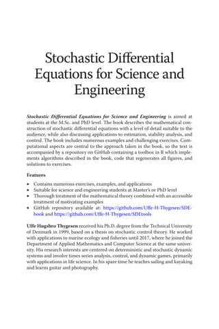


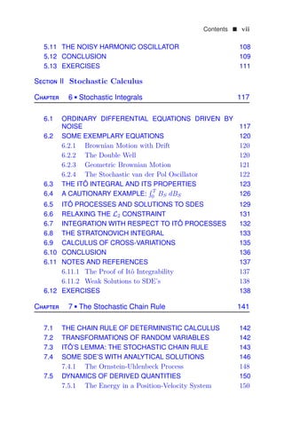


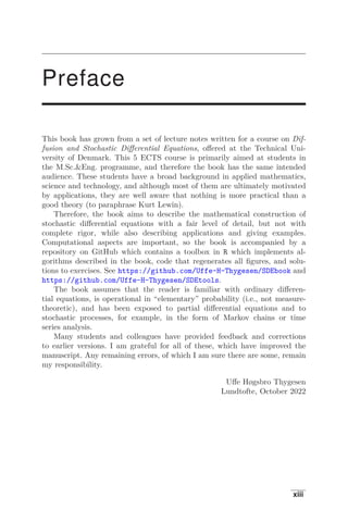

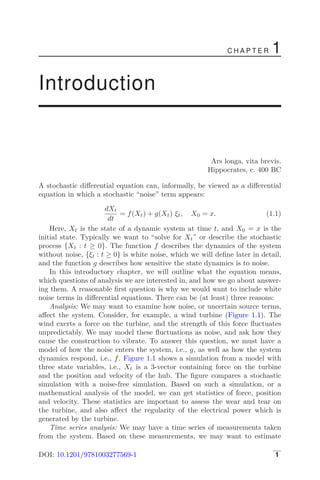
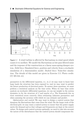

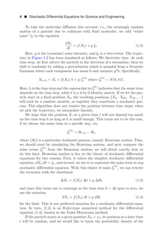
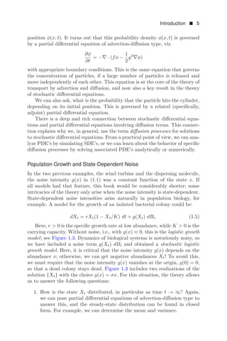


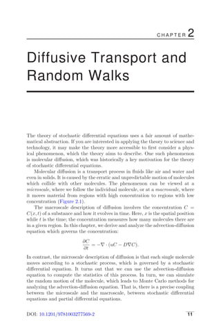
![12 Stochastic Differential Equations for Science and Engineering
Figure 2.1 Diffusion in a container in two dimensions. Top panels: Con-
centration fields. Bottom panels: Position of 100 molecules. Left panels:
Initially, the solute is concentrated at the center. Right panels: After
some time, the solute is less concentrated. The bottom right panel also
includes the trajectory of one molecule; notice its irregular appearance.
2.1 DIFFUSIVE TRANSPORT
In this section, we model how a substance spreads in space due to molecular
diffusion. Think of smoke in still air, or dye in still water. The substance is
distributed over a one-dimensional space R. Let μt([a, b]) denote the amount
of material present in the interval [a, b] at time t. Mathematically, this μt is
a measure. We may measure the substance in terms of number of molecules
or moles, or in terms of mass, but we choose to let μt be dimensionless. We
assume that μt admits a density, which is the concentration C(·, t) of the
substance, so that the amount of material present in any interval [a, b] can be
found as the integral of the concentration over the interval:
μt([a, b]) =
b
a
C(x, t) dx.
The density has unit per length; if the underlying space had been two or three
dimensional, then C would have unit per length squared or cubed, i.e., per
area or per volume. The objective of this section is to pose a partial differential
equation, the diffusion equation (2.3), which governs the time evolution of this
concentration C.](https://image.slidesharecdn.com/24320362-250520225118-652c6346/85/Stochastic-Differential-Equations-For-Science-And-Engineering-Uffe-Hgsbro-Thygesen-31-320.jpg)
![Diffusive Transport and Random Walks 13
C
x
a b
μ
Ja
Jb
Figure 2.2 Conservation in one dimension. The total mass in the interval
[a, b] is μt([a, b]) =
b
a C(x, t) dx, corresponding to the area of the shaded
region. The net flow into the interval [a, b] is J(a) − J(b).
2.1.1 The Conservation Equation
We first establish the conservation equation
∂C
∂t
+
∂J
∂x
= 0, (2.1)
which expresses that mass is redistributed in space by continuous movements,
but neither created, lost, nor teleported instantaneously between separated
regions in space. To see that this equation holds, note that transport may
then be quantified with a flux J(x, t), which is the net amount of material
that crosses the point x per unit time, from left to right. The flux has physical
dimension “per time”. Then, the amount of material in the interval [a, b] is
only changed by the net influx at the two endpoints, i.e.,
d
dt
μt([a, b]) = J(a, t) − J(b, t).
See Figure 2.2. Assume that the flux J is differentiable in x, then
J(a, t) − J(b, t) = −
b
a
∂J
∂x
(x, t) dx.
On the other hand, since μt is given as an integral, we can use the Leibniz
integral rule to find the rate of change by differentiating under the integral
sign:
d
dt
μt([a, b]) =
b
a
∂C
∂t
(x, t) dx.
Here, we assume that C is smooth so that the Leibniz integral rule applies.
Combining these two expressions for the rate of change of material in [a, b],
we obtain: b
a
∂C
∂t
(x, t) +
∂J
∂x
(x, t)
dx = 0.](https://image.slidesharecdn.com/24320362-250520225118-652c6346/85/Stochastic-Differential-Equations-For-Science-And-Engineering-Uffe-Hgsbro-Thygesen-32-320.jpg)
![14 Stochastic Differential Equations for Science and Engineering
Since the interval [a, b] is arbitrary, we can conclude that the integrand is
identically 0, or
∂C
∂t
(x, t) +
∂J
∂x
(x, t) = 0.
This is known as the conservation equation. To obtain a more compact nota-
tion, we often omit the arguments (x, t), and we use a dot (as in Ċ) for time
derivative and a prime (as in J
) for spatial derivative. Thus, we can state the
conservation equation compactly as
Ċ + J
= 0.
2.1.2 Fick’s Laws
Fick’s first law for diffusion states that the diffusive flux is proportional to the
concentration gradient:
J(x, t) = −D
∂C
∂x
(x, t) or simply J = −DC
. (2.2)
This means that the diffusion will move matter from regions of high concen-
tration to regions of low concentration. The constant of proportionality, D,
is termed the diffusivity and has dimensions area per time (also when the
underlying space has more than one dimension). The diffusivity depends on
the diffusing substance, the background material it is diffusing in, and the
temperature. See Table 2.1 for examples of diffusivities.
Fick’s first law (2.2) is empirical but consistent with a microscopic model
of molecule motion, as we will soon see. Combining Fick’s first law with the
conservation equation (2.1) gives Fick’s second law, the diffusion equation:
Ċ = (DC
)
. (2.3)
This law predicts, for example, that the concentration will decrease at a peak,
i.e., where C
= 0 and C
0. In many physical situations, the diffusivity D
is constant in space. In this case, we may write Fick’s second law as
Ċ = DC
when D is constant in space, (2.4)
i.e., the rate of increase of concentration is proportional to the spatial curva-
ture of the concentration. However, constant diffusivity is a special situation,
and the general form of the diffusion equation is (2.3).
TABLE 2.1 Examples of Diffusivities
Process Diffusivity [m2
/s]
Smoke particle in air at room temperature 2 × 10⁻⁵
Salt ions in water at room temperature 1 × 10⁻⁹
Carbon atoms in iron at 1250 K 2 × 10−11](https://image.slidesharecdn.com/24320362-250520225118-652c6346/85/Stochastic-Differential-Equations-For-Science-And-Engineering-Uffe-Hgsbro-Thygesen-33-320.jpg)
![Diffusive Transport and Random Walks 15
Biography: Adolph Eugen Fick (1829–1901)
A German pioneer in biophysics with a background
in mathematics, physics, and medicine. Interested
in transport in muscle tissue, he used the transport
of salt in water as a convenient model system. In
a sequence of papers around 1855, he reported on
experiments as well as a theoretical model of trans-
port, namely Fick’s laws, which were derived as an
analogy to the conduction of heat.
Exercise 2.1: For the situation in Figure 2.2, will the amount of material in
the interval [a, b] increase or decrease in time? Assume that (2.4) applies, i.e.,
the transport is diffusive and the diffusivity D is constant in space.
For the diffusion equation to admit a unique solution, we need an initial
condition C(x, 0) and spatial boundary conditions. Typical boundary condi-
tions either fix the concentration C at the boundary, i.e., Dirichlet conditions,
or the flux J. In the latter case, since the flux J = uC−D∇C involves both the
concentration C and its gradient ∇C, the resulting condition is of Robin type.
In many situations, the domain is unbounded so that the boundary condition
concerns the limit |x| → ∞.
2.1.3 Diffusive Spread of a Point Source
We now turn to an important situation where the diffusion equation admits
a simple solution in closed form: We take the spatial domain to be the entire
real line R, we consider a diffusivity D which is constant in space and time,
and we assume that the fluxes vanish in the limit |x| → ∞. Consider the initial
condition that one unit of material is located at position x0, i.e.,
C(x, 0) = δ(x − x0),
where δ is the Dirac delta. The solution is then a Gaussian bell curve:
C(x, t) =
1
√
2Dt
φ
x − x0
√
2Dt
. (2.5)
Here, φ(·) is the probability density function (p.d.f.) of a standard Gaussian
variable,
φ(x) =
1
√
2π
exp(−
1
2
x2
). (2.6)
Thus, the substance is distributed according to a Gaussian distribution with
mean x0 and standard deviation
√
2Dt; see Figure 2.3. This standard devia-
tion is a characteristic length scale of the concentration field which measures](https://image.slidesharecdn.com/24320362-250520225118-652c6346/85/Stochastic-Differential-Equations-For-Science-And-Engineering-Uffe-Hgsbro-Thygesen-34-320.jpg)
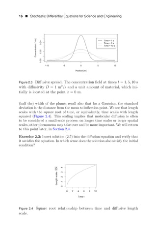
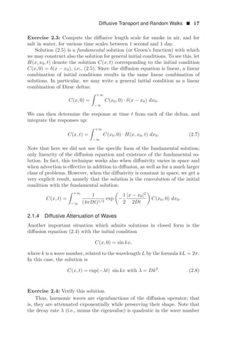
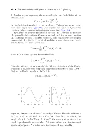
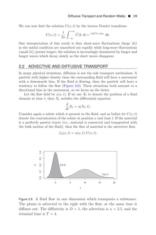
![20 Stochastic Differential Equations for Science and Engineering
If in addition molecular diffusion is in effect, then according to Fick’s first law
(2.2) this gives rise to a diffusive flux JD = −DC
. We may assume that these
two transport mechanisms operate independently, so that the total flux is the
sum of the advective and diffusive fluxes:
J(x, t) = u(x, t) C(x, t) − D(x)
∂C
∂x
(x, t),
or simply J = uC − DC
. Inserting this into the conservation equation (2.1),
we obtain the advection-diffusion equation for the concentration field:
Ċ = −(uC − DC
)
. (2.9)
A simple case is when u and D are constant, the initial condition is a Dirac
delta, C(x, 0) = δ(x − x0), where x0 is a parameter, and the flux vanishes as
|x| → ∞. Then the solution is:
C(x, t) =
1
√
4πDt
exp
−
(x − ut − x0)2
4Dt
, (2.10)
which is the probability density function of a Gaussian random variable with
mean x0 + ut and variance 2Dt. Advection shifts the mean with constant
rate, as if there had been no diffusion, and diffusion gives rise to a linearly
growing variance while preserving the Gaussian shape, as in the case of pure
diffusion (i.e., diffusion without advection). This solution is important, but
also a very special case: In general, when the flow is not constant, it will affect
the variance, and the diffusion will affect the mean.
Exercise 2.5:
1. Verify the solution (2.10).
2. Solve the advection-diffusion equation (2.9) on the real line with con-
stant u and D with the initial condition C(x, 0) = sin(kx) or, if you
prefer, C(x, 0) = exp(ikx).
2.3 DIFFUSION IN MORE THAN ONE DIMENSION
Consider again the one-dimensional situation in Figure 2.2. In n dimensions,
the interval [a, b] is replaced by a region V ⊂ Rn
. Let μt(V ) denote the amount
of the substance present in this region. This measure can be written in terms
of a volume integral of the density C:
μt(V ) =
V
C(x, t) dx.
Here x = (x1, . . . , xn) ∈ Rn
and dx is the volume of an infinitesimal volume
element. The concentration C has physical dimension “per volume”, i.e., SI](https://image.slidesharecdn.com/24320362-250520225118-652c6346/85/Stochastic-Differential-Equations-For-Science-And-Engineering-Uffe-Hgsbro-Thygesen-39-320.jpg)
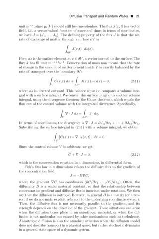
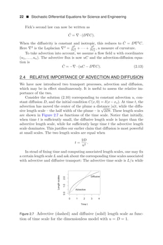
![Diffusive Transport and Random Walks 23
the diffusive time scale is L2
/2D. We define the Péclet number as the ratio
between the two:
Pe = 2
Diffusive time scale
Advective time scale
=
Lu
D
.
It is common to include factor 2 in order to obtain a simpler final expression,
but note that different authors may include different factors. Regardless of the
precise numerical value, a large Péclet number means that the diffusive time
scale is larger than the advective time scale. In this situation, advection is a
more effective transport mechanism than diffusion at the given length scale;
that is, the transport is dominated by advection. Conversely, if the Péclet
number is near 0, diffusion is more effective than advection at the given length
scale. Such considerations may suggest to simplify the model by omitting the
least significant term, and when done cautiously, this can be a good idea.
The analysis in this section has assumed that u and D were constant.
When this is not the case, it is customary to use “typical” values of u and D
to compute the Péclet number. This can be seen as a useful heuristic, but can
also be justified by the non-dimensional versions of the transport equations,
where the Péclet number enters. Of course, exactly which “typical values”
are used for u and D can be a matter of debate, but this debate most often
affects digits and not orders of magnitude. Even the order of magnitude of the
Péclet number is a useful indicator if the transport phenomenon under study
is dominated by diffusion or advection.
Example 2.4.1 Consider the advection-diffusion equation (2.13) in two di-
mensions, where the flow u(x) is around a cylinder. We non-dimensionalize
space so that the cylinder is centered at the origin and has radius 1, and non-
dimensionalize time so that the flow velocity far from the cylinder is 1. Then,
the flow is, in polar coordinates (r, θ) with x = r cos θ, y = r sin θ,
ur(r, θ) = (1 − r−2
) cos θ, uθ = −(1 + r−2
) sin θ.
This is called irrotational flow in fluid mechanics (Batchelor, 1967). A unit of
material is released at time t = 0 at position x = −3, y = −0.5. We solve the
advection-diffusion equation for t ∈ [0, 2.5] for three values of the diffusivity
D: D = 1, D = 0.1, and D = 0.01, leading to the three Péclet numbers 1, 10,
and 100. Figure 2.8 shows the solution at time t = 2.5 for the three Péclet
numbers. Notice how higher Péclet numbers (lower diffusivity D) imply a more
narrow distribution of the material.
2.5 THE MOTION OF A SINGLE MOLECULE
We can accept Fick’s first equation as an empirical fact, but we would like
to connect it to our microscopic understanding. In this section, we present a
caricature of a microscopic mechanism which can explain Fickian diffusion:
Each individual molecule moves in an erratic and unpredictable fashion, due](https://image.slidesharecdn.com/24320362-250520225118-652c6346/85/Stochastic-Differential-Equations-For-Science-And-Engineering-Uffe-Hgsbro-Thygesen-42-320.jpg)
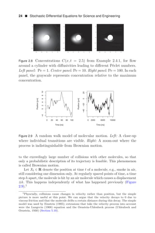
![Diffusive Transport and Random Walks 25
Biography: Robert Brown (1773–1858)
A Scottish botanist who in 1827 studied pollen im-
mersed in water under a microscope and observed
an erratic motion of the grains. Unexplained at
the time, we now attribute the motion to seem-
ingly random collision between the pollen and wa-
ter molecules. The physical phenomenon and its
mathematical model are named Brownian motion,
although many other experimentalists and theoreti-
cians contributed to our modern understanding of
the phenomenon.
In summary, the position {Xt : t ≥ 0} is a random walk:
Xt+h =
⎧
⎨
⎩
Xt + k w.p. (with probability) p,
Xt w.p. 1 − 2p,
Xt − k w.p. p.
.
Here, p ∈ (0, 1
2 ] is a parameter. The displacement in one time step, Xt+h −Xt,
has mean 0 and variance 2k2
p. Displacements over different time steps are
independent, so the central limit theorem applies. After many time steps, the
probability distribution of the displacement Xnh will be well approximated
by a Gaussian with mean 0 and variance 2k2
pn:
Xnh ∼ N(0, 2k2
pn). (2.14)
That is, Xnh will (approximately) have the probability density function
1
2k2pn
· φ(x/ 2k2pn),
where φ is still the p.d.f. of a standard Gaussian variable from (2.6). Next,
assume that we release a large number N of molecules at the origin, and that
they move independently. According to the law of large numbers, the number
of molecules present between x1 and x2 at time nh will be approximately
N
x2
x1
1
2k2pn
· φ(x/ 2k2pn) dx.
Notice that this agrees with equation (2.5), assuming that we take N = 1,
D = k2
p/h and t = nh.
We see that our cartoon model of molecular motion is consistent with the
results of the diffusion equation, if we assume that](https://image.slidesharecdn.com/24320362-250520225118-652c6346/85/Stochastic-Differential-Equations-For-Science-And-Engineering-Uffe-Hgsbro-Thygesen-44-320.jpg)
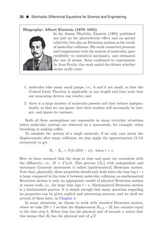
![Diffusive Transport and Random Walks 27
2.6 MONTE CARLO SIMULATION OF PARTICLE MOTION
The previous section considered diffusion only. To add advection, the mi-
croscale picture is that each particle is advected with the fluid while subject
to random collisions with other molecules which randomly perturb the parti-
cle. Thus, each particle performs a biased random walk. When the diffusivity
D and the flow u are constant in space and time, the Gaussian solution (2.10)
to the advection-diffusion equation applies. Then, a random walk model that
is consistent with the advection-diffusion equation is to sample the increments
ΔX = Xt − Xs from a Gaussian distribution
ΔX ∼ N(u · (t − s), 2D(t − s)).
Now what if the flow u = u(x, t) varies in space and time? To simulate the
trajectory of a single particle, it seems to be a reasonable heuristic to divide
the time interval [0, T] into N subintervals
0 = t0, t1, . . . , tN = T.
We first sample X0 from the initial distribution C(·, 0). Then, we sample the
remaining trajectory recursively: At each sub-interval [ti, ti+1], we approxi-
mate the flow field with a constant, namely u(Xti
, ti). This gives us:
Xti+1 ∼ N(Xti + u(Xti ) · Δti, 2D · Δti), (2.15)
where Δti = ti+1 −ti. It seems plausible that, as the time step in this recursion
goes to 0, this approximation becomes more accurate so that the p.d.f. of Xt
will approach the solution C(·, t) to the advection-diffusion equation (2.9).
This turns out to be the case, although we are far from ready to prove it.
Example 2.6.1 (Flow past a cylinder revisited) Example 2.4.1 and Fig-
ure 2.8 present solutions of the advection-diffusion equation for the case where
the flow goes around a cylinder. In the introduction, Figure 1.2 (page 3) show
a trajectory of a single molecule in the same flow. This trajectory is simulated
with the recursion (2.15), using a Péclet number of 200.
The Monte Carlo method, we have just described simulates the motion of
single molecules, chosen randomly from the ensemble. Monte Carlo simulation
can be used to compute properties of the concentration C, but can also answer
questions that are not immediately formulated using partial differential equa-
tions; for example, concerning the time a molecule spends in a region. Monte
Carlo methods are appealing in situations where analytical solutions to the
partial differential equations are not available, and when numerical solutions
are cumbersome, e.g., due to irregular geometries. Monte Carlo methods can
also be useful when other processes than transport are active, for example,
when chemical reactions take place on or between the dispersing particles.](https://image.slidesharecdn.com/24320362-250520225118-652c6346/85/Stochastic-Differential-Equations-For-Science-And-Engineering-Uffe-Hgsbro-Thygesen-46-320.jpg)
![Diffusive Transport and Random Walks 29
Factbox: [The error function] The physics literature often prefers the “er-
ror function” to the standard Gaussian cumulative distribution function.
The error function is defined as
erf(x) =
2
√
π
x
0
e−s2
ds,
and the complementary error function is
erfc(x) = 1 − erf(x) =
2
√
π
∞
x
e−s2
ds.
These are related to the standard Gaussian distribution function Φ(x) by
erfc(x) = 2 − 2Φ(
√
2x), Φ(x) = 1 −
1
2
erfc(x/
√
2).
erf(x) = 2Φ(
√
2x) − 1, Φ(x) =
1
2
+
1
2
erf(x/
√
2).
2.8 EXERCISES
Exercise 2.6:
1. Solve the diffusion equation (2.4) on the real line with a “Heaviside step”
initial condition
C(x, 0) =
0 when x 0,
1 when x 0.
.
Use boundary conditions limx→+∞ C(x, t) = 1 and limx→−∞ C(x, t) =
0.
Hint: If you cannot guess the solution, use formula (2.7) and manipulate
the integral into a form that resembles the definition of the cumulative
distribution function.
2. Consider the diffusion equation (2.4) on the positive half-line x ≥ 0
with initial condition C(x, 0) = 0 and boundary conditions C(0, t) = 1,
C(∞, t) = 0.
Hint: Utilize the solution of the previous question, and the fact that in
that question, C(0, t) = 1/2 for all t 0.
Exercise 2.7: It is useful to have simple bounds on the tail probabilities in
the Gaussian distribution, such as (Karatzas and Shreve, 1997):
x
1 + x2
φ(x) ≤ 1 − Φ(x) ≤
1
x
φ(x).](https://image.slidesharecdn.com/24320362-250520225118-652c6346/85/Stochastic-Differential-Equations-For-Science-And-Engineering-Uffe-Hgsbro-Thygesen-48-320.jpg)

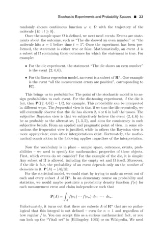
![34 Stochastic Differential Equations for Science and Engineering
to exclude such “non-measurable” subsets of Rn
: They do not correspond to
events.
In elementary probability and statistics, we tend to ignore non-measurable
subsets of Rn
, which have little relevance in applications. However, for more
complicated sample spaces Ω, which appear in the study of stochastic processes
and in particular stochastic differential equations, this difficulty cannot be
ignored: Not all subsets of the sample space can be events, and we often need
careful analysis to determined which ones are.
When not every set A ⊂ Ω can be an event, which ones should be? Some
events are required for the theory to be useful. For example, in the scalar
case Ω = R, we want intervals to correspond to events, so that the statement
ω ∈ [a, b] is an event for any a and b. Moreover, it is imperative that our
machinery of logic works: If A is an event, then the complementary set Ac
must also be an event, so that the statement “not A” is valid. Next, if also
B is an event, then the intersection A ∩ B must also be an event, so that the
statement “A and B” is valid. More generally, in stochastic processes we often
consider infinite sequences of events, for instance when analyzing convergence.
So if {Ai : i ∈ N} is a sequence of events, then the statement “for each integer
i, the statement Ai holds” should be valid. In terms of subsets of sample space
Ω, this means that A1 ∩ A2 ∩ . . . must be an event.
Let F denote the collection of events which we consider. Mathematically
speaking, the requirements on F that we have just argued for, means that F
is a σ-algebra:
Definition 3.1.1 (σ-algebra of events) Given a sample space Ω, a σ-
algebra F of events is a family of subsets of Ω for which:
1. The certain event is included, Ω ∈ F.
2. For each event A ∈ F, the complementary set Ac
is also an event,
Ac
∈ F.
3. Given a sequence of events {Ai ∈ F : i ∈ N}, it is an event that all Ai
occur, i.e., ∩iAi ∈ F.
Given a sequence of events {Ai ∈ F : i ∈ N}, also the union ∪iAi is an event.
Exercise: Verify this!. We often say, for short, that σ-algebras are characterized
by being closed under countable operations of union and intersection.
Example 3.1.1 (The Borel algebra) A specific σ-algebra which we will
encounter frequently in this book, is related to the case Ω = R. We previously
argued that the intervals [a, b] should be events for the theory to be useful in
many situations. The smallest σ-algebra which contains the intervals is called
the Borel-algebra and denoted B(R) or simply B.
The Borel algebra contains all open sets and all closed sets, as well as many
others. This collection of sets is large enough to contain the sets one encoun-
ters in practice, and the fact that the Vitali set and other non-Borel sets exist
is more an excitement to mathematicians than a nuisance to practitioners.](https://image.slidesharecdn.com/24320362-250520225118-652c6346/85/Stochastic-Differential-Equations-For-Science-And-Engineering-Uffe-Hgsbro-Thygesen-53-320.jpg)
![Stochastic Experiments and Probability Spaces 35
Biography: Félix Édouard Justin Émile Borel (1871–1956)
The French mathematician Borel was one of the
leading figures in the development of measure the-
ory. He applied measure theory to real functions of
real variables, as well as to the foundations of prob-
ability. He was also politically active, argued for a
united Europe, was Minister of the Navy, and was
imprisoned during World War II for assisting the
Resistance.
In the case Ω = Rn
, we require F to include (hyper)rectangles of the form
(a1, b1) × (a2, b2) × . . . × (an, bn), for ai, bi ∈ R and also use the name Borel-
algebra, B(Rn
), for the smallest σ-algebra that contains these hyper-rectangles.
More generally, if Ω is a topological space (i.e., we have defined a system of
open subsets of Ω), then the Borel algebra on Ω is the smallest σ-algebra of
subsets of Ω that contain all the open sets.
It is important to notice that for a given sample space Ω, there can be
several systems of events F. In many applications there is an obvious choice,
but in general, to specify a stochastic experiment, we must state not only
what can happen (i.e., Ω) but also which questions we can ask (i.e., F).
Having outcomes and events in place, we need to assign a probability P(A)
to each event A ∈ F. The way we do this must be consistent:
Definition 3.1.2 (Probability measure) A measure P is a map F →
[0, ∞] which is countably additive, i.e.: P(∪iAi) =
i P(Ai) whenever
A1, A2, . . . are mutually exclusive events (Ai ∩ Aj = ∅ for i = j). A prob-
ability measure is a measure for which P(Ω) = 1.
This definition explains why we call the sets in F measurable: F consists
exactly of those sets, for which the measure P(A) is defined. Notice that
probability is additive only for countable collections of sets, just as the σ-
algebra F must only be closed under countable unions of sets.
An event with probability 0 is called a null event. Conversely, if an event
has probability 1, then we say that this event occurs almost surely (a.s.) or
with probability 1 (w.p. 1).
Example 3.1.2 Consider the uniform distribution on [0, 1); i.e., Ω = [0, 1),
F is the Borel algebra on Ω, and probability corresponds to length, P([a, b]) =
b−a for 0 ≤ a ≤ b 1. Now, the rational numbers form a countable set Q, so
the set A = Ω∩Q is measurable and has measure P(A) = 0: When sampling a
real number uniformly from [0, 1), the probability of getting a rational number
is 0. At the same time, the rationals are dense in [0, 1) (every real number can](https://image.slidesharecdn.com/24320362-250520225118-652c6346/85/Stochastic-Differential-Equations-For-Science-And-Engineering-Uffe-Hgsbro-Thygesen-54-320.jpg)