EXACT SOLUTIONS OF SCHRÖDINGER EQUATION WITH SOLVABLE POTENTIALS FOR NON PT/P...ijrap
We have obtained explicitly the exact solutions of the Schrodinger equation with Non PT/PT symmetric
Rosen Morse II, Scarf II and Coulomb potentials. Energy eigenvalues and the corresponding
unnormalized wave functions for these systems for both Non PT and PT symmetric are also obtained using
the Nikiforov-Uvarov (NU) method.
International Journal of Mathematics and Statistics Invention (IJMSI) inventionjournals
International Journal of Mathematics and Statistics Invention (IJMSI) is an international journal intended for professionals and researchers in all fields of computer science and electronics. IJMSI publishes research articles and reviews within the whole field Mathematics and Statistics, new teaching methods, assessment, validation and the impact of new technologies and it will continue to provide information on the latest trends and developments in this ever-expanding subject. The publications of papers are selected through double peer reviewed to ensure originality, relevance, and readability. The articles published in our journal can be accessed online.
Representation of Integer Positive Number as A Sum of Natural SummandsIJERA Editor
In this paper the problem of representation of integer positive number as a sum of natural terms is considered. The new approach to calculation of number of representations is offered. Results of calculations for numbers from 1 to 500 are given. Dependence of partial contributions to total sum of number of representations is investigated. Application of results is discussed.
This paper presents concepts of Bernoulli distribution, and how it can be used as an approximation of Binomial, Poisson, and Gaussian distributions with a different approach from earlier existing literature. Due to discrete nature of the random variable X, a more appropriate method of the principle of mathematical induction (PMI) is used as an alternative approach to limiting behavior of the binomial random variable. The study proved de Moivre–Laplace theorem (convergence of binomial distribution to Gaussian distribution) to all values of p such that p ≠ 0 and p ≠ 1 using a direct approach which opposes the popular and most widely used indirect method of moment generating function.
EXPECTED NUMBER OF LEVEL CROSSINGS OF A RANDOM TRIGONOMETRIC POLYNOMIALJournal For Research
Let EN( T; Φ’ , Φ’’ ) denote the average number of real zeros of the random trigonometric polynomial T=Tn( Φ, É )= . In the interval (Φ’, Φ’’). Assuming that ak(É ) are independent random variables identically distributed according to the normal law and that bk = kp (p ≥ 0) are positive constants, we show that EN( T : 0, 2À ) ~ Outside an exceptional set of measure at most (2/ n ) where β = constant S ~ 1, S’ ~ 1. 1991 Mathematics subject classification (amer. Math. Soc.): 60 B 99.
Bound State Solution to Schrodinger Equation with Hulthen Plus Exponential Co...ijrap
In this work, we obtained an approximate bound state solution to Schrodinger with Hulthen plus
exponential Coulombic potential with centrifugal potential barrier using parametric Nikiforov-Uvarov
method. We obtained both the eigen energy and the wave functions to non -relativistic wave equations. We
implement Matlab algorithm to obtained the numerical bound state energies for various values of
adjustable screening parameter at various quantum state.. The developed potential reduces to Hulthen
potential and the numerical bound state energy conform to that of existing literature.
Necessary and Sufficient Conditions for Oscillations of Neutral Delay Differe...inventionjournals
In this paper, we discuss the oscillatory behavior of all solutions of the first order neutral delay difference equations with several positive and negative coefficients ( ) ( ) ( ) ( ) 0 , i i j j k k I J K x n p x n r x n q x n , o n n (*) where I, J and K are initial segments of natural numbers, pi , rj , qk are positive numbers, i , j are positive integers and k is a nonnegative integer for iI, jJ and kK. We establish a necessary and sufficient conditions for the oscillation of all solutions of (*) is that its characteristic equation ( 1) 1 0 j i k i j k I J K p r q has no positive roots . AMS Subject Classifications : 39A10, 39A12.
Characterization and the Kinetics of drying at the drying oven and with micro...Open Access Research Paper
The objective of this work is to contribute to valorization de Nephelium lappaceum by the characterization of kinetics of drying of seeds of Nephelium lappaceum. The seeds were dehydrated until a constant mass respectively in a drying oven and a microwawe oven. The temperatures and the powers of drying are respectively: 50, 60 and 70°C and 140, 280 and 420 W. The results show that the curves of drying of seeds of Nephelium lappaceum do not present a phase of constant kinetics. The coefficients of diffusion vary between 2.09.10-8 to 2.98. 10-8m-2/s in the interval of 50°C at 70°C and between 4.83×10-07 at 9.04×10-07 m-8/s for the powers going of 140 W with 420 W the relation between Arrhenius and a value of energy of activation of 16.49 kJ. mol-1 expressed the effect of the temperature on effective diffusivity.
"Understanding the Carbon Cycle: Processes, Human Impacts, and Strategies for...MMariSelvam4
The carbon cycle is a critical component of Earth's environmental system, governing the movement and transformation of carbon through various reservoirs, including the atmosphere, oceans, soil, and living organisms. This complex cycle involves several key processes such as photosynthesis, respiration, decomposition, and carbon sequestration, each contributing to the regulation of carbon levels on the planet.
Human activities, particularly fossil fuel combustion and deforestation, have significantly altered the natural carbon cycle, leading to increased atmospheric carbon dioxide concentrations and driving climate change. Understanding the intricacies of the carbon cycle is essential for assessing the impacts of these changes and developing effective mitigation strategies.
By studying the carbon cycle, scientists can identify carbon sources and sinks, measure carbon fluxes, and predict future trends. This knowledge is crucial for crafting policies aimed at reducing carbon emissions, enhancing carbon storage, and promoting sustainable practices. The carbon cycle's interplay with climate systems, ecosystems, and human activities underscores its importance in maintaining a stable and healthy planet.
In-depth exploration of the carbon cycle reveals the delicate balance required to sustain life and the urgent need to address anthropogenic influences. Through research, education, and policy, we can work towards restoring equilibrium in the carbon cycle and ensuring a sustainable future for generations to come.
Willie Nelson Net Worth: A Journey Through Music, Movies, and Business Venturesgreendigital
Willie Nelson is a name that resonates within the world of music and entertainment. Known for his unique voice, and masterful guitar skills. and an extraordinary career spanning several decades. Nelson has become a legend in the country music scene. But, his influence extends far beyond the realm of music. with ventures in acting, writing, activism, and business. This comprehensive article delves into Willie Nelson net worth. exploring the various facets of his career that have contributed to his large fortune.
Follow us on: Pinterest
Introduction
Willie Nelson net worth is a testament to his enduring influence and success in many fields. Born on April 29, 1933, in Abbott, Texas. Nelson's journey from a humble beginning to becoming one of the most iconic figures in American music is nothing short of inspirational. His net worth, which estimated to be around $25 million as of 2024. reflects a career that is as diverse as it is prolific.
Early Life and Musical Beginnings
Humble Origins
Willie Hugh Nelson was born during the Great Depression. a time of significant economic hardship in the United States. Raised by his grandparents. Nelson found solace and inspiration in music from an early age. His grandmother taught him to play the guitar. setting the stage for what would become an illustrious career.
First Steps in Music
Nelson's initial foray into the music industry was fraught with challenges. He moved to Nashville, Tennessee, to pursue his dreams, but success did not come . Working as a songwriter, Nelson penned hits for other artists. which helped him gain a foothold in the competitive music scene. His songwriting skills contributed to his early earnings. laying the foundation for his net worth.
Rise to Stardom
Breakthrough Albums
The 1970s marked a turning point in Willie Nelson's career. His albums "Shotgun Willie" (1973), "Red Headed Stranger" (1975). and "Stardust" (1978) received critical acclaim and commercial success. These albums not only solidified his position in the country music genre. but also introduced his music to a broader audience. The success of these albums played a crucial role in boosting Willie Nelson net worth.
Iconic Songs
Willie Nelson net worth is also attributed to his extensive catalog of hit songs. Tracks like "Blue Eyes Crying in the Rain," "On the Road Again," and "Always on My Mind" have become timeless classics. These songs have not only earned Nelson large royalties but have also ensured his continued relevance in the music industry.
Acting and Film Career
Hollywood Ventures
In addition to his music career, Willie Nelson has also made a mark in Hollywood. His distinctive personality and on-screen presence have landed him roles in several films and television shows. Notable appearances include roles in "The Electric Horseman" (1979), "Honeysuckle Rose" (1980), and "Barbarosa" (1982). These acting gigs have added a significant amount to Willie Nelson net worth.
Television Appearances
Nelson's char
WRI’s brand new “Food Service Playbook for Promoting Sustainable Food Choices” gives food service operators the very latest strategies for creating dining environments that empower consumers to choose sustainable, plant-rich dishes. This research builds off our first guide for food service, now with industry experience and insights from nearly 350 academic trials.
Climate Change All over the World .pptxsairaanwer024
Climate change refers to significant and lasting changes in the average weather patterns over periods ranging from decades to millions of years. It encompasses both global warming driven by human emissions of greenhouse gases and the resulting large-scale shifts in weather patterns. While climate change is a natural phenomenon, human activities, particularly since the Industrial Revolution, have accelerated its pace and intensity
Epcon is One of the World's leading Manufacturing Companies.EpconLP
Epcon is One of the World's leading Manufacturing Companies. With over 4000 installations worldwide, EPCON has been pioneering new techniques since 1977 that have become industry standards now. Founded in 1977, Epcon has grown from a one-man operation to a global leader in developing and manufacturing innovative air pollution control technology and industrial heating equipment.
UNDERSTANDING WHAT GREEN WASHING IS!.pdfJulietMogola
Many companies today use green washing to lure the public into thinking they are conserving the environment but in real sense they are doing more harm. There have been such several cases from very big companies here in Kenya and also globally. This ranges from various sectors from manufacturing and goes to consumer products. Educating people on greenwashing will enable people to make better choices based on their analysis and not on what they see on marketing sites.
Artificial Reefs by Kuddle Life Foundation - May 2024punit537210
Situated in Pondicherry, India, Kuddle Life Foundation is a charitable, non-profit and non-governmental organization (NGO) dedicated to improving the living standards of coastal communities and simultaneously placing a strong emphasis on the protection of marine ecosystems.
One of the key areas we work in is Artificial Reefs. This presentation captures our journey so far and our learnings. We hope you get as excited about marine conservation and artificial reefs as we are.
Please visit our website: https://kuddlelife.org
Our Instagram channel:
@kuddlelifefoundation
Our Linkedin Page:
https://www.linkedin.com/company/kuddlelifefoundation/
and write to us if you have any questions:
info@kuddlelife.org
Artificial Reefs by Kuddle Life Foundation - May 2024
lect2a.ppt
1. 1
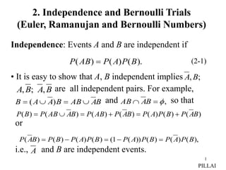
Independence: Events A and B are independent if
• It is easy to show that A, B independent implies
are all independent pairs. For example,
and so that
or
i.e., and B are independent events.
).
(
)
(
)
( B
P
A
P
AB
P (2-1)
;
,B
A
B
A
B
A ,
;
,
B
A
AB
B
A
A
B
)
( ,
B
A
AB
),
(
)
(
)
(
))
(
1
(
)
(
)
(
)
(
)
( B
P
A
P
B
P
A
P
B
P
A
P
B
P
B
A
P
)
(
)
(
)
(
)
(
)
(
)
(
)
( B
A
P
B
P
A
P
B
A
P
AB
P
B
A
AB
P
B
P
A
PILLAI
2. Independence and Bernoulli Trials
(Euler, Ramanujan and Bernoulli Numbers)
2. 2
As an application, let Ap and Aq represent the events
and
Then from (1-4)
Also
Hence it follows that Ap and Aq are independent events!
"the prime divides the number "
p
A p N
"the prime divides the number ".
q
A q N
1 1
{ } , { }
p q
P A P A
p q
1
{ } {" divides "} { } { }
p q p q
P A A P pq N P A P A
pq
(2-2)
PILLAI
3. 3
• If P(A) = 0, then since the event always, we have
and (2-1) is always satisfied. Thus the event of zero
probability is independent of every other event!
• Independent events obviously cannot be mutually
exclusive, since and A, B independent
implies Thus if A and B are independent,
the event AB cannot be the null set.
• More generally, a family of events are said to be
independent, if for every finite sub collection
we have
A
AB
,
0
)
(
0
)
(
)
(
AB
P
A
P
AB
P
0
)
(
,
0
)
(
B
P
A
P
.
0
)
(
AB
P
,
,
,
, 2
1 n
i
i
i A
A
A
n
k
i
n
k
i k
k
A
P
A
P
1
1
).
(
(2-3)
i
A
PILLAI
4. 4
• Let
a union of n independent events. Then by De-Morgan’s
law
and using their independence
Thus for any A as in (2-4)
a useful result.
We can use these results to solve an interesting number
theory problem.
,
3
2
1 n
A
A
A
A
A
(2-4)
n
A
A
A
A
2
1
.
))
(
1
(
)
(
)
(
)
(
1
1
2
1
n
i
i
n
i
i
n A
P
A
P
A
A
A
P
A
P (2-5)
,
))
(
1
(
1
)
(
1
)
(
1
n
i
i
A
P
A
P
A
P (2-6)
PILLAI
5. 5
Example 2.1 Two integers M and N are chosen at random.
What is the probability that they are relatively prime to
each other?
Solution: Since M and N are chosen at random, whether
p divides M or not does not depend on the other number N.
Thus we have
where we have used (1-4). Also from (1-10)
Observe that “M and N are relatively prime” if and only if
there exists no prime p that divides both M and N.
2
{" divides both and "}
1
{" divides "} {" divides "}
P p M N
P p M P p N
p
2
{" does divede both and "}
1
1 {" divides both and "} 1
P p not M N
P p M N
p
PILLAI
6. 6
Hence
where Xp represents the event
Hence using (2-2) and (2-5)
where we have used the Euler’s identity1
1See Appendix for a proof of Euler’s identity by Ramanujan.
2 3 5
" and are relatively prime"
M N X X X
" divides both and ".
p
X p M N
2
prime
2 2
2
prime
1
1
{" and N are relatively prime"} ( )
1 1 6
(1 ) 0.6079,
/6
1/
p
p
p
k
p
P M P X
k
PILLAI
7. 7
The same argument can be used to compute the probability
that an integer chosen at random is “square free”.
Since the event
using (2-5) we have
1
1 prime
1
1/ (1 ) .
s
s
k p
p
k
2
prime
"An integer chosen at random is square free"
{" does divide "},
p
p not N
2
2
prime prime
2 2
2
1
1
{"An integer chosen at random is square free"}
{ does divide } (1 )
1 1 6
.
/6
1/
p p
k
p
P
P p not N
k
PILLAI
8. 8
Note: To add an interesting twist to the ‘square free’ number
problem, Ramanujan has shown through elementary but
clever arguments that the inverses of the nth powers of all
‘square free’ numbers add to where (see (2-E))
Thus the sum of the inverses of the squares of ‘square free’
numbers is given by
2
/ ,
n n
S S
1
1/ .
n
n
k
S k
2
2 2 2 2 2 2 2 2 2
4
2
4 2
1 1 1 1 1 1 1 1 1
2 3 5 6 7 10 11 13 14
/6 15
1.51198.
/90
S
S
PILLAI
9. 9
Input Output
,
)
( p
A
P i
).
(
)
(
)
(
)
(
);
(
)
(
)
( 3
2
1
3
2
1 A
P
A
P
A
P
A
A
A
P
A
P
A
P
A
A
P j
i
j
i
.
3
1
i
Example 2.2: Three switches connected in parallel operate
independently. Each switch remains closed with probability
p. (a) Find the probability of receiving an input signal at the
output. (b) Find the probability that switch S1 is open given
that an input signal is received at the output.
Solution: a. Let Ai = “Switch Si is closed”. Then
Since switches operate independently, we have
Fig.2.1
PILLAI
1
s
2
s
3
s
10. 10
Let R = “input signal is received at the output”. For the
event R to occur either switch 1 or switch 2 or switch 3
must remain closed, i.e.,
(2-7)
(2-8)
(2-9)
.
3
2
1 A
A
A
R
.
3
3
)
1
(
1
)
(
)
( 3
2
3
3
2
1 p
p
p
p
A
A
A
P
R
P
).
(
)
|
(
)
(
)
|
(
)
( 1
1
1
1 A
P
A
R
P
A
P
A
R
P
R
P
,
1
)
|
( 1
A
R
P 2
3
2
1 2
)
(
)
|
( p
p
A
A
P
A
R
P
Using (2-3) - (2-6),
We can also derive (2-8) in a different manner. Since any
event and its compliment form a trivial partition, we can
always write
But and
and using these in (2-9) we obtain
,
3
3
)
1
)(
2
(
)
( 3
2
2
p
p
p
p
p
p
p
R
P
(2-10)
which agrees with (2-8).
PILLAI
11. 11
Note that the events A1, A2, A3 do not form a partition, since
they are not mutually exclusive. Obviously any two or all
three switches can be closed (or open) simultaneously.
Moreover,
b. We need From Bayes’ theorem
Because of the symmetry of the switches, we also have
.
1
)
(
)
(
)
( 3
2
1
A
P
A
P
A
P
).
|
( 1 R
A
P
.
3
3
2
2
3
3
)
1
)(
2
(
)
(
)
(
)
|
(
)
|
( 3
2
2
3
2
2
1
1
1
p
p
p
p
p
p
p
p
p
p
p
R
P
A
P
A
R
P
R
A
P
).
|
(
)
|
(
)
|
( 3
2
1 R
A
P
R
A
P
R
A
P
(2-11)
PILLAI
12. 12
Repeated Trials
Consider two independent experiments with associated
probability models (1, F1, P1) and (2, F2, P2). Let
1, 2 represent elementary events. A joint
performance of the two experiments produces an
elementary events = (, ). How to characterize an
appropriate probability to this “combined event” ?
Towards this, consider the Cartesian product space
= 1 2 generated from 1 and 2 such that if
1 and 2 , then every in is an ordered pair
of the form = (, ). To arrive at a probability model
we need to define the combined trio (, F, P).
PILLAI
13. 13
Suppose AF1 and B F2. Then A B is the set of all pairs
(, ), where A and B. Any such subset of
appears to be a legitimate event for the combined
experiment. Let F denote the field composed of all such
subsets A B together with their unions and compliments.
In this combined experiment, the probabilities of the events
A 2 and 1 B are such that
Moreover, the events A 2 and 1 B are independent for
any A F1 and B F2 . Since
we conclude using (2-12) that
).
(
)
(
),
(
)
( 2
1
1
2 B
P
B
P
A
P
A
P
(2-12)
,
)
(
)
( 1
2 B
A
B
A
(2-13)
PILLAI
14. 14
)
(
)
(
)
(
)
(
)
( 2
1
1
2 B
P
A
P
B
P
A
P
B
A
P
for all A F1 and B F2 . The assignment in (2-14) extends
to a unique probability measure on the sets in F
and defines the combined trio (, F, P).
Generalization: Given n experiments and
their associated let
represent their Cartesian product whose elementary events
are the ordered n-tuples where Events
in this combined space are of the form
where and their unions an intersections.
(2-14)
)
( 2
1 P
P
P
,
,
,
, 2
1 n
,
1
,
and n
i
P
F i
i
,
,
,
, 2
1 n
.
i
i
n
A
A
A
2
1
n
2
1
(2-15)
(2-16)
,
i
i F
A
PILLAI
15. 15
If all these n experiments are independent, and is the
probability of the event in then as before
Example 2.3: An event A has probability p of occurring in a
single trial. Find the probability that A occurs exactly k times,
k n in n trials.
Solution: Let (, F, P) be the probability model for a single
trial. The outcome of n experiments is an n-tuple
where every and as in (2-15).
The event A occurs at trial # i , if Suppose A occurs
exactly k times in .
)
( i
i A
P
i
A i
F
1 2 1 1 2 2
( ) ( ) ( ) ( ).
n n n
P A A A P A P A P A
(2-17)
,
,
,
, 0
2
1
n
(2-18)
i
0
.
A
i
PILLAI
16. 16
Then k of the belong to A, say and the
remaining are contained in its compliment in
Using (2-17), the probability of occurrence of such an is
given by
However the k occurrences of A can occur in any particular
location inside . Let represent all such
events in which A occurs exactly k times. Then
But, all these s are mutually exclusive, and equiprobable.
i
,
,
,
, 2
1 k
i
i
i
k
n .
A
.
)
(
)
(
)
(
)
(
)
(
)
(
})
({
})
({
})
({
})
({
})
,
,
,
,
,
({
)
( 2
1
2
1
0
k
n
k
k
n
k
i
i
i
i
i
i
i
i
q
p
A
P
A
P
A
P
A
P
A
P
A
P
P
P
P
P
P
P n
k
n
k
(2-19)
N
,
,
, 2
1
.
trials"
in
times
exactly
occurs
" 2
1 N
n
k
A
(2-20)
i
PILLAI
17. 17
Thus
where we have used (2-19). Recall that, starting with n
possible choices, the first object can be chosen n different
ways, and for every such choice the second one in
ways, … and the kth one ways, and this gives the
total choices for k objects out of n to be
But, this includes the choices among the k objects that
are indistinguishable for identical objects. As a result
,
)
(
)
(
)
trials"
in
times
exactly
occurs
("
0
1
0
k
n
k
N
i
i q
Np
NP
P
n
k
A
P
(2-21)
(2-22)
)
1
(
n
)
1
(
k
n
).
1
(
)
1
(
k
n
n
n
!
k
k
n
k
k
n
n
k
k
n
n
n
N
!
)!
(
!
!
)
1
(
)
1
(
PILLAI
18. 18
,
,
,
2
,
1
,
0
,
)
trials"
in
times
exactly
occurs
("
)
(
n
k
q
p
k
n
n
k
A
P
k
P
k
n
k
n
(2-23)
)
( A
)
( A
represents the number of combinations, or choices of n
identical objects taken k at a time. Using (2-22) in (2-21),
we get
a formula, due to Bernoulli.
Independent repeated experiments of this nature, where the
outcome is either a “success” or a “failure”
are characterized as Bernoulli trials, and the probability of
k successes in n trials is given by (2-23), where p
represents the probability of “success” in any one trial.
PILLAI
19. 19
Example 2.4: Toss a coin n times. Obtain the probability of
getting k heads in n trials ?
Solution: We may identify “head” with “success” (A) and
let In that case (2-23) gives the desired
probability.
Example 2.5: Consider rolling a fair die eight times. Find
the probability that either 3 or 4 shows up five times ?
Solution: In this case we can identify
Thus
and the desired probability is given by (2-23) with
and Notice that this is similar to a “biased coin”
problem.
).
(H
P
p
.
}
4
or
3
either
{
success"
" 4
3 f
f
A
,
3
1
6
1
6
1
)
(
)
(
)
( 4
3
f
P
f
P
A
P
5
,
8
k
n
.
3
/
1
p
PILLAI
20. 20
Bernoulli trial: consists of repeated independent and
identical experiments each of which has only two outcomes A
or with and The probability of exactly
k occurrences of A in n such trials is given by (2-23).
Let
Since the number of occurrences of A in n trials must be an
integer either must
occur in such an experiment. Thus
But are mutually exclusive. Thus
A .
)
( q
A
P
,
)
( p
A
P
,
,
,
2
,
1
,
0 n
k
.
trials"
in
s
occurrence
exactly
" n
k
Xk (2-24)
n
X
X
X
X or
or
or
or 2
1
0
.
1
)
( 1
0
n
X
X
X
P (2-25)
j
i X
X ,
PILLAI
21. 21
From the relation
(2-26) equals and it agrees with (2-25).
For a given n and p what is the most likely value of k ?
From Fig.2.2, the most probable value of k is that number
which maximizes in (2-23). To obtain this value,
consider the ratio
n
k
n
k
k
n
k
k
n q
p
k
n
X
P
X
X
X
P
0 0
1
0 .
)
(
)
( (2-26)
,
)
(
0
k
n
k
n
k
n
b
a
k
n
b
a
(2-27)
,
1
)
(
n
q
p
)
(k
Pn
.
2
/
1
,
12
p
n
Fig. 2.2
)
(k
Pn
k
PILLAI
22. 22
Thus if or
Thus as a function of k increases until
if it is an integer, or the largest integer less than
and (2-29) represents the most likely number of successes
(or heads) in n trials.
Example 2.6: In a Bernoulli experiment with n trials, find
the probability that the number of occurrences of A is
between and
.
1
!
!
)!
(
)!
1
(
)!
1
(
!
)
(
)
1
( 1
1
p
q
k
n
k
q
p
n
k
k
n
k
k
n
q
p
n
k
P
k
P
k
n
k
k
n
k
n
n
),
1
(
)
(
k
P
k
P n
n p
k
n
p
k )
1
(
)
1
(
.
)
1
( p
n
k
)
(k
Pn
p
n
k )
1
(
,
)
1
( p
n
(2-28)
(2-29)
1
k .
2
k
max
k
PILLAI
23. 23
Solution: With as defined in (2-24),
clearly they are mutually exclusive events. Thus
Example 2.7: Suppose 5,000 components are ordered. The
probability that a part is defective equals 0.1. What is the
probability that the total number of defective parts does not
exceed 400 ?
Solution: Let
,
,
,
2
,
1
,
0
, n
i
Xi
.
)
(
)
(
)
"
and
between
is
of
s
Occurrence
("
2
1
2
1
2
1
1 1
2
1
k
k
k
k
n
k
k
k
k
k
k
k
k q
p
k
n
X
P
X
X
X
P
k
k
A
P
(2-30)
".
components
5,000
among
defective
are
parts
"k
Yk
PILLAI
24. 24
Using (2-30), the desired probability is given by
Equation (2-31) has too many terms to compute. Clearly,
we need a technique to compute the above term in a more
efficient manner.
From (2-29), the most likely number of successes in n
trials, satisfy
or
.
)
9
.
0
(
)
1
.
0
(
5000
)
(
)
(
5000
400
0
400
0
400
1
0
k
k
k
k
k
k
Y
P
Y
Y
Y
P
(2-31)
max
k
p
n
k
p
n )
1
(
1
)
1
( max
(2-32)
,
max
n
p
p
n
k
n
q
p
(2-33)
PILLAI
25. 25
so that
From (2-34), as the ratio of the most probable
number of successes (A) to the total number of trials in a
Bernoulli experiment tends to p, the probability of
occurrence of A in a single trial. Notice that (2-34) connects
the results of an actual experiment ( ) to the axiomatic
definition of p. In this context, it is possible to obtain a more
general result as follows:
Bernoulli’s theorem: Let A denote an event whose
probability of occurrence in a single trial is p. If k denotes
the number of occurrences of A in n independent trials, then
.
lim p
n
km
n
(2-34)
,
n
.
2
n
pq
p
n
k
P
(2-35)
n
km /
PILLAI
26. 26
Equation (2-35) states that the frequency definition of
probability of an event and its axiomatic definition ( p)
can be made compatible to any degree of accuracy.
Proof: To prove Bernoulli’s theorem, we need two identities.
Note that with as in (2-23), direct computation gives
Proceeding in a similar manner, it can be shown that
n
k
)
(k
Pn
.
)
(
!
)!
1
(
)!
1
(
!
)!
1
(
!
)!
1
(
)!
(
!
!
)!
(
!
)
(
1
1
1
0
1
1
1
0
1
1
1
0
np
q
p
np
q
p
i
i
n
n
np
q
p
i
i
n
n
q
p
k
k
n
n
q
p
k
k
n
n
k
k
P
k
n
i
n
i
n
i
i
n
i
n
i
k
n
k
n
k
n
k
k
n
k
n
k
n
(2-36)
.
)!
1
(
)!
(
!
)!
2
(
)!
(
!
)!
1
(
)!
(
!
)
(
2
2
1
2
1
0
2
npq
p
n
q
p
k
k
n
n
q
p
k
k
n
n
q
p
k
k
n
n
k
k
P
k
k
n
k
n
k
k
n
k
n
k
n
k
k
n
k
n
k
n
(2-37)
PILLAI
27. 27
Returning to (2-35), note that
which in turn is equivalent to
Using (2-36)-(2-37), the left side of (2-39) can be expanded
to give
Alternatively, the left side of (2-39) can be expressed as
,
)
(
to
equivalent
is 2
2
2
n
np
k
p
n
k
(2-38)
.
)
(
)
(
)
( 2
2
0
2
2
0
2
n
k
P
n
k
P
np
k n
n
k
n
n
k
(2-39)
.
2
)
(
2
)
(
)
(
)
(
2
2
2
2
2
2
0
0
2
0
2
npq
p
n
np
np
npq
p
n
p
n
k
P
k
np
k
P
k
k
P
np
k n
n
k
n
n
k
n
n
k
(2-40)
.
)
(
)
(
)
(
)
(
)
(
)
(
)
(
)
(
)
(
2
2
2
2
2
2
2
0
2
n
np
k
P
n
k
P
n
k
P
np
k
k
P
np
k
k
P
np
k
k
P
np
k
n
n
np
k
n
n
np
k
n
n
np
k
n
n
np
k
n
n
k
(2-41)
PILLAI
28. 28
Using (2-40) in (2-41), we get the desired result
Note that for a given can be made arbitrarily
small by letting n become large. Thus for very large n, we
can make the fractional occurrence (relative frequency)
of the event A as close to the actual probability p of the
event A in a single trial. Thus the theorem states that the
probability of event A from the axiomatic framework can be
computed from the relative frequency definition quite
accurately, provided the number of experiments are large
enough. Since is the most likely value of k in n trials,
from the above discussion, as the plots of tends
to concentrate more and more around in (2-32).
.
2
n
pq
p
n
k
P
(2-42)
2
/
,
0
n
pq
n
k
max
k
,
n )
(k
Pn
max
k
PILLAI
29. 29
Next we present an example that illustrates the usefulness of
“simple textbook examples” to practical problems of interest:
Example 2.8 : Day-trading strategy : A box contains n
randomly numbered balls (not 1 through n but arbitrary
numbers including numbers greater than n). Suppose
a fraction of those balls are initially
drawn one by one with replacement while noting the numbers
on those balls. The drawing is allowed to continue until
a ball is drawn with a number larger than the first m numbers.
Determine the fraction p to be initially drawn, so as to
maximize the probability of drawing the largest among the
n numbers using this strategy.
Solution: Let “ drawn ball has the largest
number among all n balls, and the largest among the
say ; 1
m np p
st
k k
X )
1
(
PILLAI
30. 30
first k balls is in the group of first m balls, k > m.” (2.43)
Note that is of the form
where
A = “largest among the first k balls is in the group of first
m balls drawn”
and
B = “(k+1)st ball has the largest number among all n balls”.
Notice that A and B are independent events, and hence
Where m = np represents the fraction of balls to be initially
drawn. This gives
P (“selected ball has the largest number among all balls”)
k
X ,
A B
.
1
1
)
(
)
(
)
(
k
p
k
np
n
k
m
n
B
P
A
P
X
P k
(2-44)
1 1
1 1
( ) ln
ln .
n n n n
k np
np
k m k m
P X p p p k
k k
p p
(2-45)
31. 31
Maximization of the desired probability in (2-45) with
respect to p gives
or
From (2-45), the maximum value for the desired probability
of drawing the largest number equals 0.3679 also.
Interestingly the above strategy can be used to “play the
stock market”.
Suppose one gets into the market and decides to stay
up to 100 days. The stock values fluctuate day by day, and
the important question is when to get out?
According to the above strategy, one should get out
0
)
ln
1
(
)
ln
(
p
p
p
dp
d
1
0.3679.
p e
(2-46)
PILLAI
32. 32
at the first opportunity after 37 days, when the stock value
exceeds the maximum among the first 37 days. In that case
the probability of hitting the top value over 100 days for the
stock is also about 37%. Of course, the above argument
assumes that the stock values over the period of interest are
randomly fluctuating without exhibiting any other trend.
Interestingly, such is the case if we consider shorter time
frames such as inter-day trading.
In summary if one must day-trade, then a possible strategy
might be to get in at 9.30 AM, and get out any time after
12 noon (9.30 AM + 0.3679 6.5 hrs = 11.54 AM to be
precise) at the first peak that exceeds the peak value between
9.30 AM and 12 noon. In that case chances are about 37%
that one hits the absolute top value for that day! (disclaimer :
Trade at your own risk)
PILLAI
33. 33
PILLAI
We conclude this lecture with a variation of the Game of
craps discussed in Example 3-16, Text.
Example 2.9: Game of craps using biased dice:
From Example 3.16, Text, the probability of
winning the game of craps is 0.492929 for the player.
Thus the game is slightly advantageous to the house. This
conclusion of course assumes that the two dice in question
are perfect cubes. Suppose that is not the case.
Let us assume that the two dice are slightly loaded in such
a manner so that the faces 1, 2 and 3 appear with probability
and faces 4, 5 and 6 appear with probability
for each dice. If T represents the combined
total for the two dice (following Text notation), we get
1
6 0
,
1
6
34. 34
PILLAI
2
4
2 2
5
2 2
6
7
1
6
1 1
36 6
1 1
36 6
{ 4} {(1,3),(2,2),(1,3)} 3( )
{ 5} {(1,4),(2,3),(3,2),(4,1)} 2( ) 2( )
{ 6} {(1,5),(2,4),(3,3),(4,2),(5,1)} 4( ) ( )
{ 7} {(1,6),(2,5),(3,4),(4,3),(5,2),(6,1
p P T P
p P T P
p P T P
p P T P
2
2 2
8
2 2
9
2
10
11
1
36
1 1
36 6
1 1
36 6
1
6
1
6
)} 6( )
{ 8} {(2,6),(3,5),(4,4),(5,3),(6,2)} 4( ) ( )
{ 9} {(3,6),(4,5),(5,4),(6,3)} 2( ) 2( )
{ 10} {(4,6),(5,5),(6,4)} 3( )
{ 11} {(5,6),(6,5)} 2(
p P T P
p P T P
p P T P
p P T P
2
) .
(Note that “(1,3)” above represents the event “the first dice
shows face 1, and the second dice shows face 3” etc.)
For we get the following Table:
0.01,
35. 35
PILLAI
T = k 4 5 6 7 8 9 10 11
pk = P{T = k} 0.0706 0.1044 0.1353 0.1661 0.1419 0.1178 0.0936 0.0624
This gives the probability of win on the first throw to be
(use (3-56), Text)
and the probability of win by throwing a carry-over to be
(use (3-58)-(3-59), Text)
Thus
Although perfect dice gives rise to an unfavorable game,
1 ( 7) ( 11) 0.2285
P P T P T
(2-47)
2
10
2
4 7
7
0.2717
k
k k
k
p
p p
P
(2-48)
1 2
{winning the game} 0.5002
P P P
(2-49)
36. 36
PILLAI
a slight loading of the dice turns the fortunes around in
favor of the player! (Not an exciting conclusion as far as
the casinos are concerned).
Even if we let the two dice to have different loading
factors and (for the situation described above), similar
conclusions do follow. For example,
gives (show this)
Once again the game is in favor of the player!
Although the advantage is very modest in each play, from
Bernoulli’s theorem the cumulative effect can be quite
significant when a large number of game are played.
All the more reason for the casinos to keep the dice in
perfect shape.
1
2
1 2
0.01 and 0.005
{winning the game} 0.5015.
P (2-50)
37. 37
In summary, small chance variations in each game
of craps can lead to significant counter-intuitive changes
when a large number of games are played. What appears
to be a favorable game for the house may indeed become
an unfavorable game, and when played repeatedly can lead
to unpleasant outcomes.
PILLAI
38. 38
Appendix: Euler’s Identity
S. Ramanujan in one of his early papers (J. of Indian
Math Soc; V, 1913) starts with the clever observation that
if are numbers less than unity where
the subscripts are the series of prime
numbers, then1
Notice that the terms in (2-A) are arranged in such a way
that the product obtained by multiplying the subscripts are
the series of all natural numbers Clearly,
(2-A) follows by observing that the natural numbers
1The relation (2-A) is ancient.
2 3 5 7 11
, , , , ,
a a a a a
2,3,5,7,11,
2,3,4,5,6,7,8,9, .
2 3 2 2 5
2 3 5 7
2 3 7 2 2 2 3 3
1 1 1 1
1
1 1 1 1
.
a a a a a
a a a a
a a a a a a a a
(2-A)
PILLAI
39. 39
are formed by multiplying primes and their powers.
Ramanujan uses (2-A) to derive a variety of
interesting identities including the Euler’s identity that
follows by letting in
(2-A). This gives the Euler identity
The sum on the right side in (2-B) can be related to the
Bernoulli numbers (for s even).
Bernoulli numbers are positive rational numbers
defined through the power series expansion of the even
function Thus if we write
then
2 3 5
1/2 , 1/3 , 1/5 ,
s s s
a a a
1
prime 1
1
(1 ) 1/ .
s
s
p n
p
n
(2-B)
2 cot( / 2).
x x
PILLAI
1 2 3 4 5
1 1 1 1 1
6 30 42 30 66
, , , , , .
B B B B B
2 4 6
1 2 3
cot( /2) 1
2 2! 4! 6!
x x x x
x B B B
(2-C)
40. 40
By direct manipulation of (2-C) we also obtain
so that the Bernoulli numbers may be defined through
(2-D) as well. Further
which gives
Thus1
1The series can be summed using the Fourier series expansion of a periodic ramp
signal as well.
6
2 4
3
1 2
1
1 2 2! 4! 6!
x
B x
x x B x B x
e
2 1 2 1 2 4
2
0 0
2 2 2 2 2
1
4 ( )
2(2 )! 1 1 1 1
(2 ) 1 2 3 4
n n x x
x
n
n n n n n
x
e
B n dx x e e dx
n
2 4
2 4
1 1
1/ ; 1/ etc.
6 90
k k
k k
2
1
1/
k
k
PILLAI
(2-D)
2
2
2
1
(2 )
1/
2(2 )!
n
n n
n
k
B
S k
n
(2-E)