Read Anytime AnywhereEasy Ebook Downloads at ebookmeta.com
Learning Ray, 5th Early Release Max Pumperla
https://ebookmeta.com/product/learning-ray-5th-early-
release-max-pumperla/
OR CLICK HERE
DOWLOAD EBOOK
Visit and Get More Ebook Downloads Instantly at https://ebookmeta.com
3.
With Early Releaseebooks, you get books in their earliest
form—the author’s raw and unedited content as they write—
so you can take advantage of these technologies long before
the official release of these titles.
Max Pumperla, Edward Oakes, and Richard Liaw
Learning Ray
Flexible Distributed Python for Data Science
Boston Farnham Sebastopol Tokyo
Beijing Boston Farnham Sebastopol Tokyo
Beijing
Table of Contents
1.An Overview of Ray. . . . . . . . . . . . . . . . . . . . . . . . . . . . . . . . . . . . . . . . . . . . . . . . . . . . . . . . . . 7
What Is Ray? 8
What Led to Ray? 8
Flexible Workloads in Python and Reinforcement Learning 10
Three Layers: Core, Libraries and Ecosystem 11
A Distributed Computing Framework 11
A Suite of Data Science Libraries 14
Machine Learning and the Data Science Workflow 14
Data Processing with Ray Data 17
Model Training 19
Hyperparameter Tuning 22
Model Serving 24
A Growing Ecosystem 26
How Ray Integrates and Extends 26
Ray as Distributed Interface 27
Summary 27
2. Getting Started With Ray Core. . . . . . . . . . . . . . . . . . . . . . . . . . . . . . . . . . . . . . . . . . . . . . . . 29
An Introduction To Ray Core 29
A First Example Using the Ray API 30
An Overview of the Ray Core API 40
Design Principles 41
Understanding Ray System Components 42
Scheduling and Executing Work on a Node 42
The Head Node 45
Distributed Scheduling and Execution 46
Summary 48
iii
6.
3. Building YourFirst Distributed Application. . . . . . . . . . . . . . . . . . . . . . . . . . . . . . . . . . . . . 49
Setting Up A Simple Maze Problem 50
Building a Simulation 55
Training a Reinforcement Learning Model 58
Building a Distributed Ray App 62
Recapping RL Terminology 67
Summary 68
4. Reinforcement Learning with Ray RLlib. . . . . . . . . . . . . . . . . . . . . . . . . . . . . . . . . . . . . . . . 69
An Overview of RLlib 70
Getting Started With RLlib 71
Building A Gym Environment 71
Running the RLlib CLI 73
Using the RLlib Python API 74
Configuring RLlib Experiments 81
Resource Configuration 81
Debugging and Logging Configuration 82
Rollout Worker and Evaluation Configuration 82
Environment Configuration 83
Working With RLlib Environments 84
An Overview of RLlib Environments 84
Working with Multiple Agents 85
Working with Policy Servers and Clients 90
Advanced Concepts 92
Building an Advanced Environment 93
Applying Curriculum Learning 94
Working with Offline Data 96
Other Advanced Topics 97
Summary 98
5. Hyperparameter Optimization with Ray Tune. . . . . . . . . . . . . . . . . . . . . . . . . . . . . . . . . . 99
Tuning Hyperparameters 100
Building a random search example with Ray 100
Why is HPO hard? 102
An introduction to Tune 103
How does Tune work? 104
Configuring and running Tune 108
Machine Learning with Tune 113
Using RLlib with Tune 113
Tuning Keras Models 114
Summary 116
iv | Table of Contents
7.
6. Distributed Trainingwith Ray Train. . . . . . . . . . . . . . . . . . . . . . . . . . . . . . . . . . . . . . . . . . 119
The Basics of Distributed Model Training 119
Introduction to Ray Train 120
Creating an End-To-End Example for Ray Train 121
Preprocessors in Ray Train 123
Usage of Preprocessors 123
Serialization of Preprocessors 123
Trainers in Ray Train 124
Distributed Training for Gradient Boosted Trees 124
Distributed Training for Deep Learning 125
Scaling Out Training with Ray Train Trainers 127
Connecting Data to Distributed Training 128
Ray Train Features 130
Checkpoints 130
Callbacks 130
Integration with Ray Tune 131
Exporting Models 132
Some Caveats 133
7. Data Processing with Ray. . . . . . . . . . . . . . . . . . . . . . . . . . . . . . . . . . . . . . . . . . . . . . . . . . . 135
Ray Datasets 136
An Overview of Datasets 136
Datasets Basics 137
Computing Over Datasets 140
Dataset Pipelines 142
Example: Parallel SGD from Scratch 145
External Library Integrations 148
Overview 148
Dask on Ray 149
Building an ML Pipeline 151
Background 151
End-to-End Example: Predicting Big Tips in Nyc Taxi Rides 152
Table of Contents | v
9.
CHAPTER 1
An Overviewof Ray
A distributed system is one in which the failure of a computer you didn’t even know
existed can render your own computer unusable.
—Leslie Lamport
A Note for Early Release Readers
With Early Release ebooks, you get books in their earliest form—the author’s raw and
unedited content as they write—so you can take advantage of these technologies long
before the official release of these titles.
One of the reasons we need efficient distributed computing is that we’re collecting
ever more data with a large variety at increasing speeds. The storage systems, data
processing and analytics engines that have emerged in the last decade are crucially
important to the success of many companies. Interestingly, most “big data” technolo‐
gies are built for and operated by (data) engineers, that are in charge of data collec‐
tion and processing tasks. The rationale is to free up data scientists to do what they’re
best at. As a data science practitioner you might want to focus on training complex
machine learning models, running efficient hyperparameter selection, building
entirely new and custom models or simulations, or serving your models to showcase
them. At the same time you simply might have to scale them to a compute cluster. To
do that, the distributed system of your choice needs to support all of these fine-
grained “big compute” tasks, potentially on specialized hardware. Ideally, it also fits
into the big data tool chain you’re using and is fast enough to meet your latency
requirements. In other words, distributed computing has to be powerful and flexible
enough for complex data science workloads — and Ray can help you with that.
7
10.
Python is likelythe most popular language for data science today, and it’s certainly
the one I find the most useful for my daily work. By now it’s over 30 years old, but has
a still growing and active community. The rich PyData ecosystem is an essential part
of a data scientist’s toolbox. How can you make sure to scale out your workloads
while still leveraging the tools you need? That’s a difficult problem, especially since
communities can’t be forced to just toss their toolbox, or programming language.
That means distributed computing tools for data science have to be built for their
existing community.
What Is Ray?
What I like about Ray is that it checks all the above boxes. It’s a flexible distributed
computing framework build for the Python data science community. Ray is easy to
get started and keeps simple things simple. Its core API is as lean as it gets and helps
you reason effectively about the distributed programs you want to write. You can effi‐
ciently parallelize Python programs on your laptop, and run the code you tested
locally on a cluster practically without any changes. Its high-level libraries are easy to
configure and can seamlessly be used together. Some of them, like Ray’s reinforce‐
ment learning library, would have a bright future as standalone projects, distributed
or not. While Ray’s core is built in C++, it’s been a Python-first framework since day
one, integrates with many important data science tools, and can count on a growing
ecosystem.
Distributed Python is not new, and Ray is not the first framework in this space (nor
will it be the last), but it is special in what it has to offer. Ray is particularly strong
when you combine several of its modules and have custom, machine learning heavy
workloads that would be difficult to implement otherwise. It makes distributed com‐
puting easy enough to run your complex workloads flexibly by leveraging the Python
tools you know and want to use. In other words, by learning Ray you get to know
flexible distributed Python for data science.
In this chapter you’ll get a first glimpse at what Ray can do for you. We will discuss
the three layers that make up Ray, namely its core engine, its high-level libraries and
its ecosystem. Throughout the chapter we’ll show you first code examples to give you
a feel for Ray, but we defer any in-depth treatment of Ray’s APIs and components to
later chapters. You can view this chapter as an overview of the whole book as well.
What Led to Ray?
Programming distributed systems is hard. It requires specific knowledge and experi‐
ence you might not have. Ideally, such systems get out of your way and provide
abstractions to let you focus on your job. But in practice “all non-trivial abstractions,
to some degree, are leaky” (Spolsky), and getting clusters of computers to do what
8 | Chapter 1: An Overview of Ray
11.
1 Moore’s Lawheld for a long time, but there might be signs that it’s slowing down. We’re not here to argue it,
though. What’s important is not that our computers generally keep getting faster, but the relation to the
amount of compute we need.
you want is undoubtedly difficult. Many software systems require resources that far
exceed what single servers can do. Even if one server was enough, modern systems
need to be failsafe and provide features like high availability. That means your appli‐
cations might have to run on multiple machines, or even datacenters, just to make
sure they’re running reliably.
Even if you’re not too familiar with machine learning (ML) or more generally artifi‐
cial intelligence (AI) as such, you must have heard of recent breakthroughs in the
field. To name just two, systems like Deepmind’s AlphaFold for solving the protein
folding problem, or OpenAI’s Codex that’s helping software developers with the tedi‐
ous parts of their job, have made the news lately. You might also have heard that ML
systems generally require large amounts of data to be trained. OpenAI has shown
exponential growth in compute needed to train AI models in their paper “AI and
Compute”. The operations needed for AI systems in their study is measured in peta‐
flops (thousands of trillion operations per second), and has been doubling every 3.4
months since 2012.
Compare this to Moore’s Law1
, which states that the number of transistors in comput‐
ers would double every two years. Even if you’re bullish on Moore’s law, you can see
how there’s a clear need for distributed computing in ML. You should also under‐
stand that many tasks in ML can be naturally decomposed to run in parallel. So, why
not speed things up if you can?
Distributed computing is generally perceived as hard. But why is that? Shouldn’t it be
realistic to find good abstractions to run your code on clusters, without having to
constantly think about individual machines and how they interoperate? What if we
specifically focused on AI workloads?
Researchers at RISELab at UC Berkeley created Ray to address these questions. None
of the tools existing at the time met their needs. They were looking for easy ways to
speed up their workloads by distributing them to compute clusters. The workloads
they had in mind were quite flexible in nature and didn’t fit into the analytics engines
available. At the same time, RISELab wanted to build a system that took care of how
the work was distributed. With reasonable default behaviors in place, researchers
should be able to focus on their work. And ideally they should have access to all their
favorite tools in Python. For this reason, Ray was built with an emphasis on high-
performance and heterogeneous workloads. Anyscale, the company behind Ray, is
building a managed Ray Platform and offers hosted solutions for your Ray applica‐
tions. Let’s have a look at an example of what kinds of applications Ray was designed
for.
What Led to Ray? | 9
12.
Flexible Workloads inPython and Reinforcement Learning
One of my favorite apps on my phone can automatically classify or “label” individual
plants in our garden. It works by simply showing it a picture of the plant in question.
That’s immensely helpful, as I’m terrible at distinguishing them all. (I’m not bragging
about the size of my garden, I’m just bad at it.) In the last couple of years we’ve seen a
surge of impressive applications like that.
Ultimately, the promise of AI is to build intelligent agents that go far beyond classify‐
ing objects. Imagine an AI application that not only knows your plants, but can take
care of to them, too. Such an application would have to
• Operate in dynamic environments (like the change of seasons)
• React to changes in the environment (like a heavy storm or pests attacking your
plants)
• Take sequences of actions (like watering and fertilizing plants)
• Accomplish long-term goals (like prioritizing plant health)
By observing its environment such an AI would also learn to explore the possible
actions it could take and come up with better solutions over time. If you feel like this
example is artificial or too far out, it’s not difficult to come up with examples on your
own that share all the above requirements. Think of managing and optimizing a sup‐
ply chain, strategically restocking a warehouse considering fluctuating demands, or
orchestrating the processing steps in an assembly line. Another famous example of
what you could expect from an AI would be Stephen Wozniak’s famous “Coffee Test”.
If you’re invited to a friend’s house, you can navigate to the kitchen, spot the coffee
machine and all necessary ingredients, figure out how to brew a cup of coffee, and sit
down to enjoy it. A machine should be able to do the same, except the last part might
be a bit of a stretch. What other examples can you think of?
You can frame all the above requirements naturally in a subfield of machine learning
called reinforcement learning (RL). We’ve dedicated all of Chapter 4 to RL. For now,
it’s enough to understand that it’s about agents interacting with their environment by
observing it and emitting actions. In RL, agents evaluate their environments by attrib‐
uting a reward (e.g., how healthy is my plant on a scale from 1 to 10). The term “rein‐
forcement” comes from the fact that agents will hopefully learn to seek out behaviour
that leads to good outcomes (high reward), and shy away from punishing situations
(low or negative reward). The interaction of agents with their environment is usually
modeled by creating a computer simulation of it. These simulations can become com‐
plicated quite quickly, as you might imagine from the examples we’ve given.
10 | Chapter 1: An Overview of Ray
13.
2 For theexperts among you, I don’t claim that RL is the answer. RL is just a paradigm that naturally fits into
this discussion of AI goals.
3 This is a Python book, so we’ll exclusively focus on it. But you should at least know that Ray also has a Java
API, which at this point is less mature than its Python equivalent.
We don’t have gardening robots like the one I’ve sketched yet. And we don’t know
which AI paradigm will get us there.2
What I do know is that the world is full of com‐
plex, dynamic and interesting examples that we need to tackle. For that we need com‐
putational frameworks that help us do that, and Ray was built to do exactly that.
RISELab created Ray to build and run complex AI applications at scale, and rein‐
forcement learning has been an integral part of Ray from the start.
Three Layers: Core, Libraries and Ecosystem
Now that you know why Ray was built and what its creators had in mind, let’s look at
the three layers of Ray.
• A low-level, distributed computing framework for Python with a concise core
API.3
• A set of high-level libraries for data science built and maintained by the creators
of Ray.
• A growing ecosystem of integrations and partnerships with other notable
projects.
There’s a lot to unpack here, and we’ll look into each of these layers individually in the
remainder of this chapter. You can imagine Ray’s core engine with its API at the cen‐
ter of things, on which everything else builds. Ray’s data science libraries build on top
of it. In practice, most data scientists will use these higher level libraries directly and
won’t often need to resort to the core API. The growing number of third-party inte‐
grations for Ray is another great entrypoint for experienced practitioners. Let’s look
into each one of the layers one by one.
A Distributed Computing Framework
At its core, Ray is a distributed computing framework. We’ll provide you with just the
basic terminology here, and talk about Ray’s architecture in depth in Chapter 2. In
short, Ray sets up and manages clusters of computers so that you can run distributed
tasks on them. A ray cluster consists of nodes that are connected to each other via a
network. You program against the so-called driver, the program root, which lives on
the head node. The driver can run jobs, that is a collection of tasks, that are run on the
nodes in the cluster. Specifically, the individual tasks of a job are run on worker pro‐
A Distributed Computing Framework | 11
14.
4 We’re usingRay version 1.9.0 at this point, as it’s the latest version available as of this writing.
cesses on worker nodes. Figure Figure 1-1 illustrates the basic structure of a Ray clus‐
ter.
Figure 1-1. The basic components of a Ray cluster
What’s interesting is that a Ray cluster can also be a local cluster, i.e. a cluster consist‐
ing just of your own computer. In this case, there’s just one node, namely the head
node, which has the driver process and some worker processes. The default number
of worker processes is the number of CPUs available on your machine.
With that knowledge at hand, it’s time to get your hands dirty and run your first local
Ray cluster. Installing Ray4
on any of the major operating systems should work seam‐
lessly using pip:
pip install "ray[rllib, serve, tune]"==1.9.0
With a simple pip install ray you would have installed just the very basics of Ray.
Since we want to explore some advanced features, we installed the “extras” rllib,
serve and tune, which we’ll discuss in a bit. Depending on your system configuration
you may not need the quotation marks in the above installation command.
Next, go ahead and start a Python session. You could use the ipython interpreter,
which I find to be the most suitable environment for following along simple exam‐
ples. If you don’t feel like typing in the commands yourself, you can also jump into
the jupyter notebook for this chapter and run the code there. The choice is up to you,
but in any case please remember to use Python version 3.7 or later. In your Python
session you can now easily import and initialize Ray as follows:
12 | Chapter 1: An Overview of Ray
15.
Example 1-1.
import ray
ray.init()
Withthose two lines of code you’ve started a Ray cluster on your local machine. This
cluster can utilize all the cores available on your computer as workers. In this case
you didn’t provide any arguments to the init function. If you wanted to run Ray on a
“real” cluster, you’d have to pass more arguments to init. The rest of your code
would stay the same.
After running this code you should see output of the following form (we use ellipses
to remove the clutter):
... INFO services.py:1263 -- View the Ray dashboard at http://127.0.0.1:8265
{'node_ip_address': '192.168.1.41',
'raylet_ip_address': '192.168.1.41',
'redis_address': '192.168.1.41:6379',
'object_store_address': '.../sockets/plasma_store',
'raylet_socket_name': '.../sockets/raylet',
'webui_url': '127.0.0.1:8265',
'session_dir': '...',
'metrics_export_port': 61794,
'node_id': '...'}
This indicates that your Ray cluster is up and running. As you can see from the first
line of the output, Ray comes with its own, pre-packaged dashboard. In all likelihood
you can check it out at http://127.0.0.1:8265, unless your output shows a different
port. If you want you can take your time to explore the dashboard for a little. For
instance, you should see all your CPU cores listed and the total utilization of your
(trivial) Ray application. We’ll come back to the dashboard in later chapters.
We’re not quite ready to dive into all the details of a Ray cluster here. To jump ahead
just a little, you might see the raylet_ip_address, which is a reference to a so-called
Raylet, which is responsible for scheduling tasks on your worker nodes. Each Raylet
has a store for distributed objects, which is hinted at by the object_store_address
above. Once tasks are scheduled, they get executed by worker processes. In Chapter 2
you’ll get a much better understanding of all these components and how they make
up a Ray cluster.
Before moving on, we should also briefly mention that the Ray core API is very acces‐
sible and easy to use. But since it is also a rather low-level interface, it takes time to
build interesting examples with it. Chapter 2 has an extensive first example to get you
started with the Ray core API, and in Chapter 3 you’ll see how to build a more inter‐
esting Ray application for reinforcement learning.
A Distributed Computing Framework | 13
16.
5 I neverliked the categorization of data science as an intersection of disciplines, like maths, coding and busi‐
ness. Ultimately, that doesn’t tell you what practitioners do. It doesn’t do a cook justice to tell them they sit at
the intersection of agriculture, thermodynamics and human relations. It’s not wrong, but also not very help‐
ful.
6 As a fun exercise, I recommend reading Paul Graham’s famous “Hackers and Painters” essay on this topic and
replace “computer science” with “data science”. What would hacking 2.0 be?
Right now your Ray cluster doesn’t do much, but that’s about to change. After giving
you a quick introduction to the data science workflow in the following section, you’ll
run your first concrete Ray examples.
A Suite of Data Science Libraries
Moving on to the second layer of Ray, in this section we’ll introduce all the data sci‐
ence libraries that Ray comes with. To do so, let’s first take a bird’s eye view on what it
means to do data science. Once you understand this context, it’s much easier to place
Ray’s higher-level libraries and see how they can be useful to you. If you have a good
idea of the data science process, you can safely skip ahead to section “Data Processing
with Ray Data” on page 17.
Machine Learning and the Data Science Workflow
The somewhat elusive term “data science” (DS) evolved quite a bit in recent years,
and you can find many definitions of varying usefulness online.5
To me, it’s the prac‐
tice of gaining insights and building real-world applications by leveraging data. That’s
quite a broad definition, and you don’t have to agree with me. My point is that data
science is an inherently practical and applied field that centers around building and
understanding things, which makes fairly little sense in a purely academic context. In
that sense, describing practitioners of this field as “data scientists” is about as bad of a
misnomer as describing hackers as “computer scientists”.6
Since you are familiar with Python and hopefully bring a certain craftsmanship atti‐
tude with you, we can approach the Ray’s data science libraries from a very pragmatic
angle. Doing data science in practice is an iterative process that goes something like
this:
Requirements engineering
You talk to stakeholders to identify the problems you need to solve and clarify the
requirements for this project.
Data collection
Then you source, collect and inspect the data.
14 | Chapter 1: An Overview of Ray
17.
Data processing
Afterwards youprocess the data such that you can tackle the problem.
Model building
You then move on to build a model (in the broadest sense) using the data. That
could be a dashboard with important metrics, a visualisation, or a machine learn‐
ing model, among many other things.
Model evaluation
The next step is to evaluate your model against the requirements in the first step.
Deployment
If all goes well (it likely doesn’t), you deploy your solution in a production envi‐
ronment. You should understand this as an ongoing process that needs to be
monitored, not as a one-off step.
Otherwise, you need to circle back and start from the top. The most likely outcome is
that you need to improve your solution in various ways, even after initial deployment.
Machine learning is not necessarily part of this process, but you can see how building
smart applications or gaining insights might benefit from ML. Building a face detec‐
tion app into your social media platform, for better or worse, might be one example
of that. When the data science process just described explicitly involves building
machine learning models, you can further specify some steps:
Data processing
To train machine learning models, you need data in a format that is understood
by your ML model. The process of transforming and selecting what data should
be fed into your model is often called feature engineering. This step can be messy.
You’ll benefit a lot if you can rely on common tools to do the job.
Model training
In ML you need to train your algorithms on data that got processed in the last
step. This includes selecting the right algorithm for the job, and it helps if you can
choose from a wide variety.
Hyperparameter tuning
Machine learning models have parameters that are tuned in the model training
step. Most ML models also have another set of parameters, called hyperparame‐
ters that can be modified prior to training. These parameters can heavily influ‐
ence the performance of your resulting ML model and need to be tuned properly.
There are good tools to help automate that process.
Model serving
Trained models need to be deployed. To serve a model means to make it available
to whoever needs access by whatever means necessary. In prototypes, you often
A Suite of Data Science Libraries | 15
18.
use simple HTTPservers, but there are many specialised software packages for
ML model serving.
This list is by no means exhaustive. Don’t worry if you’ve never gone through these
steps or struggle with the terminology, we’ll come back to this in much more detail in
later chapters. If you want to understand more about the holistic view of the data sci‐
ence process when building machine learning applications, the book Building
Machine Learning Powered Applications is dedicated to it entirely.
Figure Figure 1-2 gives an overview of the steps we just discussed:
Figure 1-2. An overview of the data science experimentation workflow using machine
learning
At this point you might be wondering how any of this relates to Ray. The good news
is that Ray has a dedicated library for each of the four ML-specific tasks above, cover‐
ing data processing, model training, hyperparameter tuning and model serving. And
the way Ray is designed, all these libraries are distributed by construction. Let’s walk
through each of them one-by-one.
16 | Chapter 1: An Overview of Ray
19.
Data Processing withRay Data
The first high-level library of Ray we talk about is called “Ray Data”. This library con‐
tains a data structure aptly called Dataset, a multitude of connectors for loading data
from various formats and systems, an API for transforming such datasets, a way to
build data processing pipelines with them, and many integrations with other data
processing frameworks. The Dataset abstraction builds on the powerful Arrow
framework.
To use Ray Data, you need to install Arrow for Python, for instance by running pip
install pyarrow. We’ll now discuss a simple example that creates a distributed Data
set on your local Ray cluster from a Python data structure. Specifically, you’ll create a
dataset from a Python dictionary containing a string name and an integer-valued data
for 10000 entries:
Example 1-2.
import ray
items = [{"name": str(i), "data": i} for i in range(10000)]
ds = ray.data.from_items(items)
ds.show(5)
Creating a Dataset by using from_items from the ray.data module.
Printing the first 10 items of the Dataset.
To show a Dataset means to print some of its values. You should see precisely 5 so-
called ArrowRow elements on your command line, like this:
ArrowRow({'name': '0', 'data': 0})
ArrowRow({'name': '1', 'data': 1})
ArrowRow({'name': '2', 'data': 2})
ArrowRow({'name': '3', 'data': 3})
ArrowRow({'name': '4', 'data': 4})
Great, now you have some distributed rows, but what can you do with that data? The
Dataset API bets heavily on functional programming, as it is very well suited for data
transformations. Even though Python 3 made a point of hiding some of its functional
programming capabilities, you’re probably familiar with functionality such as map,
filter and others. If not, it’s easy enough to pick up. map takes each element of your
dataset and transforms is into something else, in parallel. filter removes data points
according to a boolean filter function. And the slightly more elaborate flat_map first
maps values similarly to map, but then also “flattens” the result. For instance, if map
would produce a list of lists, flat_map would flatten out the nested lists and give you
A Suite of Data Science Libraries | 17
20.
just a list.Equipped with these three functional API calls, let’s see how easily you can
transform your dataset ds:
Example 1-3. Transforming a Dataset with common functional programming routines
squares = ds.map(lambda x: x["data"] ** 2)
evens = squares.filter(lambda x: x % 2 == 0)
evens.count()
cubes = evens.flat_map(lambda x: [x, x**3])
sample = cubes.take(10)
print(sample)
We map each row of ds to only keep the square value of its data entry.
Then we filter the squares to only keep even numbers (a total of 5000 ele‐
ments).
We then use flat_map to augment the remaining values with their respective
cubes.
To take a total of 10 values means to leave Ray and return a Python list with
these values that we can print.
The drawback of Dataset transformations is that each step gets executed synchro‐
nously. In example Example 1-3 this is a non-issue, but for complex tasks that e.g.
mix reading files and processing data, you want an execution that can overlap indi‐
vidual tasks. DatasetPipeline does exactly that. Let’s rewrite the last example into a
pipeline.
Example 1-4.
pipe = ds.window()
result = pipe
.map(lambda x: x["data"] ** 2)
.filter(lambda x: x % 2 == 0)
.flat_map(lambda x: [x, x**3])
result.show(10)
You can turn a Dataset into a pipeline by calling .window() on it.
Pipeline steps can be chained to yield the same result as before.
18 | Chapter 1: An Overview of Ray
21.
There’s a lotmore to be said about Ray Data, especially its integration with notable
data processing systems, but we’ll have to defer an in-depth discussion until Chap‐
ter 7.
Model Training
Moving on to the next set of libraries, let’s look at the distributed training capabilities
of Ray. For that, you have access to two libraries. One is dedicated to reinforcement
learning specifically, the other one has a different scope and is aimed primarily at
supervised learning tasks.
Reinforcement learning with Ray RLlib
Let’s start with Ray RLlib for reinforcement learning. This library is powered by the
modern ML frameworks TensorFlow and PyTorch, and you can choose which one to
use. Both frameworks seem to converge more and more conceptually, so you can pick
the one you like most without losing much in the process. Throughout the book we
use TensorFlow for consistency. Go ahead and install it with pip install tensor
flow right now.
One of the easiest ways to run examples with RLlib is to use the command line tool
rllib, which we’ve already implicitly installed earlier with pip. Once you run more
complex examples in Chapter 4, you will mostly rely on its Python API, but for now
we just want to get a first taste of running RL experiments.
We’ll look at a fairly classical control problem of balancing a pendulum. Imagine you
have a pendulum like the one in figure Figure 1-3, fixed at as single point and subject
to gravity. You can manipulate that pendulum by giving it a push from the left or the
right. If you assert just the right amount of force, the pendulum might remain in an
upright position. That’s our goal - and the question is whether we can teach a rein‐
forcement learning algorithm to do so for us.
A Suite of Data Science Libraries | 19
22.
Figure 1-3. Controllinga simple pendulum by asserting force to the left or the right
Specifically, we want to train a reinforcement learning agent that can push to the left
or right, thereby acting on its environment (manipulating the pendulum) to reach the
“upright position” goal for which it will be rewarded. To tackle this problem with Ray
RLlib, store the following content in a file called pendulum.yml.
Example 1-5.
# pendulum.yml
pendulumppo:
env: Pendulum-v1
run: PPO
checkpoint_freq: 5
stop:
episode_reward_mean: 800
config:
lambda: 0.1
gamma: 0.95
lr: 0.0003
num_sgd_iter: 6
The Pendulum-v1 environment simulates the pendulum problem we just
described.
We use a powerful RL algorithm called Proximal Policy Optimization, or PPO.
20 | Chapter 1: An Overview of Ray
23.
After every five“training iterations” we checkpoint a model.
Once we reach a reward of -800 , we stop the experiment.
The PPO needs some RL-specific configuration to make it work for this problem.
The details of this configuration file don’t matter much at this point, don’t get distrac‐
ted by them. The important part is that you specify the built-in Pendulum-v1 environ‐
ment and sufficient RL-specific configuration to ensure the training procedure works.
The configuration is a simplified version of one of Ray’s tuned examples. We chose
this one because it doesn’t require any special hardware and finishes in a matter of
minutes. If your computer is powerful enough, you can try to run the tuned example
as well, which should yield much better results. To train this pendulum example you
can now simply run:
rllib train -f pendulum.yml
If you want, you can check the output of this Ray program and see how the different
metrics evolve during the training procedure. In case you don’t want to create this file
on your own, and want to run an experiment which gives you much better results,
you can also run this:
curl https://raw.githubusercontent.com/maxpumperla/learning_ray/main/notebooks/pendulum.yml -o pen
rllib train -f pendulum.yml
In any case, assuming the training program finished, we can now check how well it
worked. To visualize the trained pendulum you need to install one more Python
library with pip install pyglet. The only other thing you need to figure out is
where Ray stored your training progress. When you run rllib train for an experi‐
ment, Ray will create a unique experiment ID for you and stores results in a sub-
folder of ~/ray-results by default. For the training configuration we used, you
should see a folder with results that looks like ~/ray_results/pendulum-ppo/
PPO_Pendulum-v1_<experiment_id>. During the training procedure intermediate
model checkpoints get generated in the same folder. For instance, I have a folder on
my machine called:
~/ray_results/pendulum-ppo/PPO_Pendulum-v1_20cbf_00000_0_2021-09-24_15-20-03/checkpoint_000029/ch
Once you figured out the experiment ID and chose a checkpoint ID (as a rule of
thumb the larger the ID, the better the results), you can evaluate the training perfor‐
mance of your pendulum training run like this:
rllib evaluate
~/ray_results/pendulum-ppo/PPO_Pendulum-v1_<experiment_id>/checkpoint_0000<cp-id>/checkpoint-<cp
--run PPO --env Pendulum-v1 --steps 2000
You should see an animation of a pendulum controlled by an agent that looks like
figure Figure 1-3. Since we opted for a quick training procedure instead of maximiz‐
A Suite of Data Science Libraries | 21
24.
ing performance, youshould see the agent struggle with the pendulum exercise. We
could have done much better, and if you’re interested to scan Ray’s tuned examples
for the Pendulum-v1 environment, you’ll find an abundance of solutions to this exer‐
cise. The point of this example was to show you how simple it can be to train and
evaluate reinforcement learning tasks with RLlib, using just two command line calls
to rllib.
Distributed training with Ray Train
Ray RLlib is dedicated to reinforcement learning, but what do you do if you need to
train models for other types of machine learning, like supervised learning? You can
use another Ray library for distributed training in this case, called Ray Train. At this
point, we don’t have built up enough knowledge of frameworks such as TensorFlow
to give you a concrete and informative example for Ray Train. We’ll discuss all of that
in Chapter 6, when it’s time to. But we can at least roughly sketch what a distributed
training “wrapper” for an ML model would look like, which is simple enough con‐
ceptually:
Example 1-6.
from ray.train import Trainer
def training_function():
pass
trainer = Trainer(backend="tensorflow", num_workers=4)
trainer.start()
results = trainer.run(training_function)
trainer.shutdown()
First, define your ML model training function. We simply pass here.
Then initialize a Trainer instance with TensorFlow as the backend.
Lastly, scale out your training function on a Ray cluster.
If you’re interested in distributed training, you could jump ahead to Chapter 6.
Hyperparameter Tuning
Naming things is hard, but the Ray team hit the spot with Ray Tune, which you can
use to tune all sorts of parameters. Specifically, it was built to find good hyperparame‐
ters for machine learning models. The typical setup is as follows:
22 | Chapter 1: An Overview of Ray
25.
• You wantto run an extremely computationally expensive training function. In
ML it’s not uncommon to run training procedures that take days, if not weeks,
but let’s say you’re dealing with just a couple of minutes.
• As result of training, you compute a so-called objective function. Usually you
either want to maximize your gains or minimize your losses in terms of perfor‐
mance of your experiment.
• The tricky bit is that your training function might depend on certain parameters,
hyperparameters, that influence the value of your objective function.
• You may have a hunch what individual hyperparameters should be, but tuning
them all can be difficult. Even if you can restrict these parameters to a sensible
range, it’s usually prohibitive to test a wide range of combinations. Your training
function is simply too expensive.
What can you do to efficiently sample hyperparameters and get “good enough” results
on your objective? The field concerned with solving this problem is called hyperpara‐
meter optimization (HPO), and Ray Tune has an enormous suite of algorithms for
tackling it. Let’s look at a first example of Ray Tune used for the situation we just
explained. The focus is yet again on Ray and its API, and not on a specific ML task
(which we simply simulate for now).
Example 1-7. Minimizing an objective for an expensive training function with Ray Tune
from ray import tune
import math
import time
def training_function(config):
x, y = config["x"], config["y"]
time.sleep(10)
score = objective(x, y)
tune.report(score=score)
def objective(x, y):
return math.sqrt((x**2 + y**2)/2)
result = tune.run(
training_function,
config={
"x": tune.grid_search([-1, -.5, 0, .5, 1]),
"y": tune.grid_search([-1, -.5, 0, .5, 1])
})
print(result.get_best_config(metric="score", mode="min"))
A Suite of Data Science Libraries | 23
26.
We simulate anexpensive training function that depends on two hyperparame‐
ters x and y, read from a config.
After sleeping for 5 seconds to simulate training and computing the objective we
report back the score to tune.
The objective computes the mean of the squares of x and y and returns the
square root of this term. This type of objective is fairly common in ML.
We then use tune.run to initialize hyperparameter optimization on our train
ing_function.
A key part is to provide a parameter space for x and y for tune to search over.
The Tune example in Example 1-7 finds the best possible choices of parameters x and
y for a training_function with a given objective we want to minimize. Even
though the objective function might look a little intimidating at first, since we com‐
pute the sum of squares of x and y, all values will be non-negative. That means the
smallest value is obtained at x=0 and y=0 which evaluates the objective function to 0.
We do a so-called grid search over all possible parameter combinations. As we explic‐
itly pass in five possible values for both x and y that’s a total of 25 combinations that
get fed into the training function. Since we instruct training_function to sleep for
10 seconds, testing all combinations of hyperparameters sequentially would take
more than four minutes total. Since Ray is smart about parallelizing this workload, on
my laptop this whole experiment only takes about 35 seconds. Now, imagine each
training run would have taken several hours, and we’d have 20 instead of two hyper‐
parameters. That makes grid search infeasible, especially if you don’t have educated
guesses on the parameter range. In such situations you’ll have to use more elaborate
HPO methods from Ray Tune, as discussed in Chapter 5.
Model Serving
The last of Ray’s high-level libraries we’ll discuss specializes on model serving and is
simply called Ray Serve. To see an example of it in action, you need a trained ML
model to serve. Luckily, nowadays you can find many interesting models on the inter‐
net that have already been trained for you. For instance, Hugging Face has a variety of
models available for you to download directly in Python. The model we’ll use is a lan‐
guage model called GPT-2 that takes text as input and produces text to continue or
complete the input. For example, you can prompt a question and GPT-2 will try to
complete it.
24 | Chapter 1: An Overview of Ray
27.
Serving such amodel is a good way to make it accessible. You may not now how to
load and run a TensorFlow model on your computer, but you do now how to ask a
question in plain English. Model serving hides the implementation details of a solu‐
tion and lets users focus on providing inputs and understanding outputs of a model.
To proceed, make sure to run pip install transformers to install the Hugging Face
library that has the model we want to use. With that we can now import and start an
instance of Ray’s serve library, load and deploy a GPT-2 model and ask it for the
meaning of life, like so:
Example 1-8.
from ray import serve
from transformers import pipeline
import requests
serve.start()
@serve.deployment
def model(request):
language_model = pipeline("text-generation", model="gpt2")
query = request.query_params["query"]
return language_model(query, max_length=100)
model.deploy()
query = "What's the meaning of life?"
response = requests.get(f"http://localhost:8000/model?query={query}")
print(response.text)
We start serve locally.
The @serve.deployment decorator turns a function with a request parameter
into a serve deployment.
Loading language_model inside the model function for every request is ineffi‐
cient, but it’s the quickest way to show you a deployment.
We ask the model to give us at most 100 characters to continue our query.
Then we formally deploy the model so that it can start receiving requests over
HTTP.
We use the indispensable requests library to get a response for any question you
might have.
A Suite of Data Science Libraries | 25
28.
7 Spark hasbeen created by another lab in Berkeley, AMPLab. The internet is full of blog posts claiming that
Ray should therefore be seen as a replacement of Spark. It’s better to think of them as tools with different
strengths that are both likely here to stay.
In ??? you will learn how to properly deploy models in various scenarios, but for now
I encourage you to play around with this example and test different queries. Running
the last two lines of code repeatedly will give you different answers practically every
time. Here’s a darkly poetic gem, raising more questions, that I queried on my
machine and slightly censored for underaged readers:
[{
"generated_text": "What's the meaning of life?nn
Is there one way or another of living?nn
How does it feel to be trapped in a relationship?nn
How can it be changed before it's too late?
What did we call it in our time?nn
Where do we fit within this world and what are we going to live for?nn
My life as a person has been shaped by the love I've received from others."
}]
This concludes our whirlwind tour of Ray’s data science libraries, the second of Ray’s
layers. Before we wrap up this chapter, let’s have a very brief look at the third layer,
the growing ecosystem around Ray.
A Growing Ecosystem
Ray’s high-level libraries are powerful and deserve a much deeper treatment through‐
out the book. While their usefulness for the data science experimentation lifecycle is
undeniable, I also don’t want to give off the impression that Ray is all you need from
now on. In fact, I believe the best and most successful frameworks are the ones that
integrate well with existing solutions and ideas. It’s better to focus on your core
strengths and leverage other tools for what’s missing in your solution. There’s usually
no reason to re-invent the wheel.
How Ray Integrates and Extends
To give you an example for how Ray integrates with other tools, consider that Ray
Data is a relatively new addition to its libraries. If you want to boil it down, and
maybe oversimplify a little, Ray is a compute-first framework. In contrast, distributed
frameworks like Apache Spark7
or Dask can be considered data-first. Pretty much
anything you do with Spark starts with the definition of a distributed dataset and
transformations thereof. Dask bets on bringing common data structures like Pandas
dataframes or Numpy arrays to a distributed setup. Both are immensely powerful in
their own regard, and we’ll give you a more detailed and fair comparison to Ray
26 | Chapter 1: An Overview of Ray
29.
8 Before thedeep learning framework Keras became an official part of a corporate flagship, it started out as a
convenient API specification for various lower-level frameworks such as Theano, CNTK, or TensorFlow. In
that sense Ray RLlib has the chance to become Keras for RL. Ray Tune might just be Keras for HPO. The
missing piece for more adoption is probably a more elegant API for both.
9 Note that “Ray Train” has been called “raysgd” in older versions of Ray, and does not have a new logo yet.
in ???. The gist of it is that Ray Data does not attempt to replace these tools. Instead, it
integrates well with both. As you’ll come to see, that’s a common theme with Ray.
Ray as Distributed Interface
One aspect of Ray that’s vastly understated in my eyes is that its libraries seamlessly
integrate common tools as backends. Ray often creates common interfaces, instead of
trying to create new standards8
. These interfaces allow you to run tasks in a dis‐
tributed fashion, a property most of the respective backends don’t have, or not to the
same extent. For instance, Ray RLlib and Train are backed by the full power of
TensorFlow and PyTorch. Ray Tune supports algorithms from practically every nota‐
ble HPO tool available, including Hyperopt, Optuna, Nevergrad, Ax, SigOpt and
many others. None of these tools are distributed by default, but Tune unifies them in
a common interface. Ray Serve can be used with frameworks such as FastAPI, and
Ray Data is backed by Arrow and comes with many integrations to other frameworks,
such as Spark and Dask. Overall this seems to be a robust design pattern that can be
used to extend current Ray projects or integrate new backends in the future.
Summary
To sum up what we’ve discussed in this chapter, Figure 1-4 gives you an overview of
the three layers of Ray as we laid them out. Ray’s core distributed execution engine
sits at the center of the framework. For practical data science workflows you can use
Ray Data for data processing, Ray RLlib for reinforcement learning, Ray Train for dis‐
tributed model training, Ray Tune for hyperparameter tuning and Ray Serve for
model serving. You’ve seen examples for each of these libraries and have an idea of
what their APIs entail. On top of that, Ray’s ecosystem has many extensions that we’ll
look more into later on. Maybe you can already spot a few tools you know and like in
Figure 1-49
?
Summary | 27
30.
Figure 1-4. Rayin three layers: its core API, the libraries RLlib, Tune, Ray Train, Ray
Serve, Ray Data, and some of the many third-party integrations
28 | Chapter 1: An Overview of Ray
31.
CHAPTER 2
Getting StartedWith Ray Core
A Note for Early Release Readers
With Early Release ebooks, you get books in their earliest form—the author’s raw and
unedited content as they write—so you can take advantage of these technologies long
before the official release of these titles.
For a book on distributed Python, it’s not without a certain irony that Python on its
own is largely ineffective for distributed computing. Its interpreter is effectively single
threaded which makes it difficult to, for example, leverage multiple CPUs on the same
machine, let alone a whole cluster of machines, using plain Python. That means you
need extra tooling, and luckily the Python ecosystem has some options for you. For
instance, libraries like multiprocessing can help you distribute work on a single
machine, but not beyond.
In this chapter you’ll understand how Ray core handles distributed computing by
spinning up a local cluster, and you’ll learn how to use Ray’s lean and powerful API to
parallelize some interesting computations. For instance, you’ll build an example that
runs a data-parallel task efficiently and asynchronously on Ray, in a convenient way
that’s not easily replicable with other tooling. We discuss how tasks and actors work as
distributed versions of functions and classes in Python. You’ll also learn about all the
fundamental concepts underlying Ray and what its architecture looks like. In other
words, we’ll give you a look under the hood of Ray’s engine.
An Introduction To Ray Core
The bulk of this chapter is an extended Ray core example that we’ll build together.
Many of Ray’s concepts can be explained with a good example, so that’s exactly what
29
32.
we’ll do. Asbefore, you can follow this example by typing the code yourself (which is
highly recommended), or by following the notebook for this chapter.
In Chapter 1 we’ve introduced you to the very basics of Ray clusters and showed you
how start a local cluster simply by typing
Example 2-1.
import ray
ray.init()
You’ll need a running Ray cluster to run the examples in this chapter, so make sure
you’ve started one before continuing. The goal of this section is to give you a quick
introduction to the Ray Core API, which we’ll simply refer to as the Ray API from
now on.
As a Python programmer, the great thing about the Ray API is that it hits so close to
home. It uses familiar concepts such as decorators, functions and classes to provide
you with a fast learning experience. The Ray API aims to provide a universal pro‐
gramming interface for distributed computing. That’s certainly no easy feat, but I
think Ray succeeds in this respect, as it provides you with good abstractions that are
intuitive to learn and use. Ray’s engine does all the heavy lifting for you in the back‐
ground. This design philosophy is what enables Ray to be used with existing Python
libraries and systems.
A First Example Using the Ray API
To give you an example, take the following function which retrieves and processes
data from a database. Our dummy database is a plain Python list containing the
words of the title of this book. We act as if retrieving an individual item from this
database and further processing it is expensive by letting Python sleep.
Example 2-2.
import time
database = [
"Learning", "Ray",
"Flexible", "Distributed", "Python", "for", "Data", "Science"
]
def retrieve(item):
time.sleep(item / 10.)
return item, database[item]
30 | Chapter 2: Getting Started With Ray Core
33.
A dummy databasecontaining string data with the title of this book.
We emulate a data-crunching operation that takes a long time.
Our database has eight items, from database[0] for “Learning” to database[7] for
“Science”. If we were to retrieve all items sequentially, how long should that take? For
the item with index 5 we wait for half a second (5 / 10.) and so on. In total, we can
expect a runtime of around (0+1+2+3+4+5+6+7)/10. = 2.8 seconds. Let’s see if that’s
what we actually get:
Example 2-3.
def print_runtime(input_data, start_time, decimals=1):
print(f'Runtime: {time.time() - start_time:.{decimals}f} seconds, data:')
print(*input_data, sep="n")
start = time.time()
data = [retrieve(item) for item in range(8)]
print_runtime(data, start)
We use a list comprehension to retrieve all eight items.
Then we unpack the data to print each item on its own line.
If you run this code, you should see the following output:
Runtime: 2.8 seconds, data:
(0, 'Learning')
(1, 'Ray')
(2, 'Flexible')
(3, 'Distributed')
(4, 'Python')
(5, 'for')
(6, 'Data')
(7, 'Science')
We cut off the output of the program after one decimal number. There’s a little over‐
head that brings the total closer to 2.82 seconds. On your end this might be slightly
less, or much more, depending on your computer. The important take-away is that
our naive Python implementation is not able to run this function in parallel. This
may not come as a surprise to you, but you could have at least suspected that Python
list comprehensions are more efficient in that regard. The runtime we got is pretty
much the worst case scenario, namely the 2.8 seconds we calculated prior to running
the code. If you think about it, it might even be a bit frustrating to see that a program
that essentially sleeps most of its runtime is that slow overall. Ultimately you can
blame the Global Interpreter Lock (GIL) for that, but it gets enough of it already.
An Introduction To Ray Core | 31
34.
1 I stilldon’t know how to pronounce this acronym, but I get the feeling that the same people who pronounce
GIF like “giraffe” also say GIL like “guitar”. Just pick one, or spell it out, if you feel insecure.
Python’s Global Interpreter Lock
The Global Interpreter Lock or GIL1
is undoubtedly one of the most infamous fea‐
tures of the Python language. In a nutshell it’s a lock that makes sure only one thread
on your computer can ever execute your Python code at a time. If you use multi-
threading, the threads need to take turns controlling the Python interpreter.
The GIL has been implemented for good reasons. For one, it makes memory manage‐
ment that much easier in Python. Another key advantage is that it makes single-
threaded programs quite fast. Programs that primarily use lots of system input and
output (we say they are I/O-bound), like reading files or databases, benefit as well.
One of the major downsides is that CPU-bound programs are essentially single-
threaded. In fact, CPU-bound tasks might even run faster when not using multi-
threading, as the latter incurs write-lock overheads on top of the GIL.
Given all that, the GIL might somewhat paradoxically be one of the reasons for
Python’s popularity, if you believe Larry Hastings. Interestingly, Hastings also led
(unsuccessful) efforts to remove it in a project called GILectomy, which is exactly the
kind of complicated surgery that it sounds like. The jury is still out, but Sam Gross
might just have found a way to remove the GIL in his nogil branch of Python 3.9. For
now, if you absolutely have to work around the GIL, consider using an implementa‐
tion different from CPython. CPython is Python’s standard implementation, and if
you don’t know that you’re using it, you’re definitely using it. Implementations like
Jython, IronPython or PyPy don’t have a GIL, but come with their own drawbacks.
Functions and Remote Ray Tasks
It’s reasonable to assume that such a task can benefit from parallelization. Perfectly
distributed, the runtime should not take much longer than the longest subtask,
namely 7/10. = 0.7 seconds. So, let’s see how you can extend this example to run on
Ray. To do so, you start by using the @ray.remote decorator as follows:
Example 2-4.
@ray.remote
def retrieve_task(item):
return retrieve(item)
With just this decorator we make any Python function a Ray task.
All else remains unchanged. retrieve_task just passes through to retrieve.
32 | Chapter 2: Getting Started With Ray Core
35.
2 This examplehas been adapted from Dean Wampler’s fantastic report “What is Ray?”.
In this way, the function retrieve_task becomes a so-called Ray task. That’s an
extremely convenient design choice, as you can focus on your Python code first, and
don’t have to completely change your mindset or programming paradigm to use Ray.
Note that in practice you would have simply added the @ray.remote decorator to
your original retrieve function (after all, that’s the intended use of decorators), but
we didn’t want to touch previous code to keep things as clear as possible.
Easy enough, so what do you have to change in the code that retrieves the data and
measures performance? It turns out, not much. Let’s have a look at how you’d do that:
Example 2-5. Measuring performance of your Ray task.
start = time.time()
data_references = [retrieve_task.remote(item) for item in range(8)]
data = ray.get(data_references)
print_runtime(data, start, 2)
To run retrieve_task on your local Ray cluster, you use .remote() and pass in
your data as before. You’ll get a list of object references.
To get back data, and not just Ray object references, you use ray.get.
Did you spot the differences? You have to execute your Ray task remotely using the
remote function. When tasks get executed remotely, even on your local cluster, Ray
does so asynchronously. The list items in data_references in the last code snippet do
not contain the results directly. In fact, if you check the Python type of the first item
with type(data_references[0]) you’ll see that it’s in fact an ObjectRef. These
object references correspond to futures which you need to ask the result of. This is
what the call to ray.get(...) is for.
We still want to work more on this example2
, but let’s take a step back here and recap
what we did so far. You started with a Python function and decorated it with
@ray.remote. This made your function a Ray task. Then, instead of calling the origi‐
nal function in your code straight-up, you called .remote(...) on the Ray task. The
last step was to .get(...) the results back from your Ray cluster. I think this proce‐
dure is so intuitive that I’d bet you could already create your own Ray task from
another function without having to look back at this example. Why don’t you give it a
try right now?
Coming back to our example, by using Ray tasks, what did we gain in terms of per‐
formance? On my machine the runtime clocks in at 0.71 seconds, which is just
An Introduction To Ray Core | 33
36.
slightly more thanthe longest subtask, which comes in at 0.7 seconds. That’s great
and much better than before, but we can further improve our program by leveraging
more of Ray’s API.
Using the object store with put and get
One thing you might have noticed is that in the definition of retrieve we directly
accessed items from our database. Working on a local Ray cluster this is fine, but
imagine you’re running on an actual cluster comprising several computers. How
would all those computers access the same data? Remember from Chapter 1 that in a
Ray cluster there is one head node with a driver process (running ray.init()) and
many worker nodes with worker processes executing your tasks. My laptop has a total
of 8 CPU cores, so Ray will create 8 worker processes on my one-node local cluster.
Our database is currently defined on the driver only, but the workers running your
tasks need to have access to it to run the retrieve task. Luckily, Ray provides an easy
way to share data between the driver and workers (or between workers). You can sim‐
ply use put to place your data into Ray’s distributed object store and then use get on
the workers to retrieve it as follows.
Example 2-6.
database_object_ref = ray.put(database)
@ray.remote
def retrieve_task(item):
obj_store_data = ray.get(database_object_ref)
time.sleep(item / 10.)
return item, obj_store_data[item]
put your database into the object store and receive a reference to it.
This allows your workers to get the data, no matter where they are located in the
cluster.
By using the object store this way, you can let Ray handle data access across the whole
cluster. We’ll talk about how exactly data is passed between nodes and within workers
when talking about Ray’s infrastructure. While the interaction with the object store
requires some overhead, Ray is really smart about storing the data, which gives you
performance gains when working with larger, more realistic datasets. For now, the
important part is that this step is essential in a truly distributed setting. If you like, try
to re-run Example 2-5 with this new retrieve_task function and confirm that it still
runs, as expected.
34 | Chapter 2: Getting Started With Ray Core
37.
Using Ray’s waitfunction for non-blocking calls
Note how in Example 2-5 we used ray.get(data_references) to access results. This
call is blocking, which means that our driver has to wait for all the results to be avail‐
able. That’s not a big deal in our case, the program now finishes in under a second.
But imagine processing of each data item would take several minutes. In that case you
would want to free up the driver process for other tasks, instead of sitting idly by.
Also, it would be great to process results as they come in (some finish much quicker
than others), rather than waiting for all data to be processed. One more question to
keep in mind is what happens if one of the data items can’t be retrieved as expected?
Let’s say there’s a deadlock somewhere in the database connection. In that case, the
driver will simply hang and never retrieve all items. For that reason it’s a good idea to
work with reasonable timeouts. In our scenario, we should not wait longer than 10
times the longest data retrieval task before stopping the task. Here’s how you can do
that with Ray by using wait:
Example 2-7.
start = time.time()
data_references = [retrieve_task.remote(item) for item in range(8)]
all_data = []
while len(data_references) > 0:
finished, data_references = ray.wait(data_references, num_returns=2, timeout=7.0)
data = ray.get(finished)
print_runtime(data, start, 3)
all_data.extend(data)
Instead of blocking, we loop through unfinished data_references.
We asynchronously wait for finished data with a reasonable timeout. data_ref
erences gets overridden here, to prevent an infinite loop.
We print results as they come in, namely in blocks of two.
Then we append new data to the all_data until finished.
As you can see ray.wait returns two arguments, namely finished data and futures
that still need to be processed. We use the num_returns argument, which defaults to
1, to let wait return whenever a new pair of data items is available. On my laptop this
results in the following output:
Runtime: 0.108 seconds, data:
(0, 'Learning')
(1, 'Ray')
Runtime: 0.308 seconds, data:
An Introduction To Ray Core | 35
38.
(2, 'Flexible')
(3, 'Distributed')
Runtime:0.508 seconds, data:
(4, 'Python')
(5, 'for')
Runtime: 0.709 seconds, data:
(6, 'Data')
(7, 'Science')
Note how in the while loop, instead of just printing results, we could have done many
other things, like starting entirely new tasks on other workers with the data already
retrieved up to this point.
Handling task dependencies
So far our example program has been fairly easy on a conceptual level. It consists of a
single step, namely retrieving a bunch of data. Now, imagine that once your data is
loaded you want to run a follow-up processing task on it. To be more concrete, let’s
say we want to use the result of our first retrieve task to query other, related data (pre‐
tend that you’re querying data from a different table in the same database). The fol‐
lowing code sets up such a task and runs both our retrieve_task and
follow_up_task consecutively.
Example 2-8. Running a follow-up task that depends on another Ray task
@ray.remote
def follow_up_task(retrieve_result):
original_item, _ = retrieve_result
follow_up_result = retrieve(original_item + 1)
return retrieve_result, follow_up_result
retrieve_refs = [retrieve_task.remote(item) for item in [0, 2, 4, 6]]
follow_up_refs = [follow_up_task.remote(ref) for ref in retrieve_refs]
result = [print(data) for data in ray.get(follow_up_refs)]
Using the result of retrieve_task we compute another Ray task on top of it.
Leveraging the original_item from the first task, we retrieve more data.
Then we return both the original and the follow-up data.
We pass the object references from the first task into the second task.
Running this code results in the following output.
36 | Chapter 2: Getting Started With Ray Core
39.
3 According toClarke’s third law any sufficiently advanced technology is indistinguishable from magic. For me,
this example has a bit of magic to it.
((0, 'Learning'), (1, 'Ray'))
((2, 'Flexible'), (3, 'Distributed'))
((4, 'Python'), (5, 'for'))
((6, 'Data'), (7, 'Science'))
If you don’t have a lot of experience with asynchronous programming, you might not
be impressed by Example 2-8. But I hope to convince you that it’s at least a bit sur‐
prising3
that this code snippet runs at all. So, what’s the big deal? After all, the code
reads like regular Python - a function definition and a few list comprehensions. The
point is that the function body of follow_up_task expects a Python tuple for its
input argument retrieve_result, which we unpack in the first line of the function
definition.
But by invoking [follow_up_task.remote(ref) for ref in retrieve_refs] we
do not pass in tuples to the follow-up task at all. Instead, we pass in Ray object refer‐
ences with retrieve_refs. What happens under the hood is that Ray knows that fol
low_up_task requires actual values, so internally in this task it will call ray.get to
resolve the futures. Ray builds a dependency graph for all tasks and executes them in
an order that respects the dependencies. You do not have to tell Ray explicitly when
to wait for a previous task to finish, it will infer that information for you.
The follow-up tasks will only be scheduled, once the individual retrieve tasks have
finished. If you ask me, that’s an incredible feature. In fact, if I had called
retrieve_refs something like retrieve_result, you may not even have noticed this
important detail. That’s by design. Ray wants you to focus on your work, not on the
details of cluster computing. In figure Figure 2-1 you can see the dependency graph
for the two tasks visualized.
An Introduction To Ray Core | 37
40.
4 The actormodel is an established concept in computer science, which you can find implemented e.g. in Akka
or Erlang. However, the history and specifics of actors are not relevant to our discussion.
Figure 2-1. Running two dependent tasks asynchronously and in parallel with Ray
If you feel like it, try to rewrite Example 2-8 so that it explicitly uses get on the first
task before passing values into the follow-up task. That does not only introduce more
boilerplate code, but it’s also a bit less intuitive to write and understand.
From classes to actors
Before wrapping up this example, let’s discuss one more important concept of Ray
Core. Notice how in our example everything is essentially a function. We just used
the ray.remote decorator to make some of them remote functions, and other than
that simply used plain Python. Let’s say we wanted to track how often our database
has been queried? Sure, we could simply count the results of our retrieve tasks, but is
there a better way to do this? We want to track this in a “distributed” way that will
scale. For that, Ray has the concept of actors. Actors allow you to run stateful compu‐
tations on your cluster. They can also communicate between each other4
. Much like
Ray tasks were simply decorated functions, Ray actors are decorated Python classes.
Let’s write a simple counter to track our database calls.
Example 2-9.
@ray.remote
class DataTracker:
def __init__(self):
38 | Chapter 2: Getting Started With Ray Core
41.
self._counts = 0
defincrement(self):
self._counts += 1
def counts(self):
return self._counts
We can make any Python class a Ray actor by using the same ray.remote decora‐
tor as before.
This DataTracker class is already an actor, since we equipped it with the ray.remote
decorator. This actor can track state, here just a simple counter, and its methods are
Ray tasks that get invoked precisely like we did with functions before, namely
using .remote(). Let’s see how we can modify our existing retrieve_task to incor‐
porate this new actor.
Example 2-10.
@ray.remote
def retrieve_tracker_task(item, tracker):
obj_store_data = ray.get(database_object_ref)
time.sleep(item / 10.)
tracker.increment.remote()
return item, obj_store_data[item]
tracker = DataTracker.remote()
data_references = [retrieve_tracker_task.remote(item, tracker) for item in range(8)]
data = ray.get(data_references)
print(ray.get(tracker.counts.remote()))
We pass in the tracker actor into this task.
The tracker receives an increment for each call.
We instantiate our DataTracker actor by calling .remote() on the class.
The actor gets passed into the retrieve task.
Afterwards we can get the counts state from our tracker from another remote
invocation.
Unsurprisingly, the result of this computation is in fact 8. We didn’t need actors to
compute this, but I hope you can see how useful it can be to have a mechanism to
track state across the cluster, potentially spanning multiple tasks. In fact, we could
An Introduction To Ray Core | 39
bet himself, butsimply to show his hand, in order to see whether or
not it is better than D’s.
SHOWING HANDS. It is the general usage that the hand called
must be shown first. In this case A’s hand is called, for D was the
one who called a halt on A in the betting, and stopped him from
going any further. The strict laws of the game require that both
hands must be shown, and if there are more than two in the final
call, all must be shown to the table. The excuse generally made for
not showing the losing hand is that the man with the worse hand
paid to see the better hand; but it must not be forgotten that the
man with the better hand has paid exactly the same amount, and is
equally entitled to see the worse hand. There is an excellent rule in
some clubs that a player refusing to show his hand in a call shall
refund the amount of the antes to all the other players, or pay all
the antes in the next jack pot. The rule of showing both hands is a
safeguard against collusion between two players, one of whom
might have a fairly good hand, and the other nothing; but by
mutually raising each other back and forth they could force any
other player out of the pool. The good hand could then be called
and shown, the confederate simply saying, “That is good,” and
throwing down his hand. Professionals call this system of cheating,
“raising out.”
When the hands are called and shown, the best poker hand wins,
their rank being determined by the table of values already given. In
the example just given suppose that A, on being called by D, had
shown three fours, and that D had three deuces. A would take the
entire pool, including all the antes, and the four blues and one red
staked by B after the draw. It might be that B would now discover
that he had laid down the best hand, having held three sixes. This
discovery would be of no benefit to him, for he abandoned his hand
when he declined to meet the raises of A and D.
If the hands are exactly a tie, the pool must be divided among
those who are in at the call. For instance: Two players show aces up,
and each finds his opponent’s second pair to be eights. The odd card
44.
must decide thepool; and if that card is also a tie the pool must be
divided.
If no bet is made after the draw, each player in turn throwing
down his cards, the antes are won by the last player who holds his
hand. This is usually the age, because he has the last say. If the age
has not made good his ante, it will be the dealer, and so on to the
right. There is no necessity for the fortunate player to show his
hand; the mere fact that he is the only one holding any cards is
prima facie evidence that his hand is the best. On the same
principle, the player who has made a bet or raise which no other
player will see, wins the pool without showing his hand, as he must
be the only one with cards in his hand; for when a player refuses to
see a bet he must abandon his hand, and with it all pretensions to
the pool. If he wishes to call, but has not money enough, he must
borrow it. He cannot demand a show of hands for what counters he
has, except in table stakes.
During the betting, players are at liberty to make any remarks
they see fit, and to tell as many cheerful lies about their hands as
they please. A player may even miscall his hand when he shows it;
the cards speak for themselves, just as the counters do, and what a
player says does not affect either in the slightest. If a player says: “I
raise you two blues,” the statement amounts to nothing until the
blues have been placed in the pool, and the owner’s hand removed
from them. There is no penalty if a player, during the betting, tells
his adversaries exactly what he holds; nor is he likely to lose
anything by it, for no one will believe him.
JACK POTS. The addition of jack pots has probably done more to
injure Poker than the trump signal has injured Whist. In the early
days, when poker parties were small, four players being a common
number, it was frequently the case that no one had a pair strong
enough to draw to, and such a deal was regarded as simply a waste
of time. To remedy this, it was proposed that whenever no player
came in, each should be obliged to ante an equal amount for the
next deal, and just to demonstrate that there were some good
45.
hands left inthe pack no one was allowed to draw cards until some
one had Jacks or better to draw to.
The result of this practice was to make jack pots larger than the
other pools, because every one was compelled to ante, and this
seems to have prompted those who were always wanting to increase
the stakes to devise excuses for increasing the number of jack pots.
This has been carried so far that the whole system has become a
nuisance, and has destroyed one of the finest points in the game of
Poker,—the liberty of personal judgment as to every counter put into
the pool, except the blind. The following excuses for making jack
pots are now in common use:
After a Misdeal some parties make it a jack; but the practice
should be condemned, because it puts it in the power of any
individual player to make it a jack when he deals.
The Buck is some article, such as a penknife, which is placed in
the pool at the beginning of the game, and is taken down with the
rest of the pool by whichever player wins it. When it comes to his
deal, it is a jack pot, and the buck is placed in the pool with the
dealer’s ante, to be won, taken down, and make another jack in the
same way.
The usual custom is to fix the amount of the ante in jack pots, a
red, or five whites, being the common stake. In some places it is at
the option of the holder of the buck to make the ante any amount
he pleases within the betting limit. Whichever system is adopted,
every player at the table must deposit a like amount in the pool.
Players are sometimes permitted to pass a jack; that is, not to ante
nor to take any part in the game until the jack is decided. If this is to
be allowed, it should be so understood at the beginning of the
game.
The High Hand jack pot is played whenever a hand of an agreed
value, such as a flush or a full, is shown to the board; that is, called.
In some places four of a kind calls for a round of jacks, every
player in turn making it a jack on his deal.
46.
Only Two In.It is a common custom in large parties, say six or
seven players, to make it a jack when no one but the dealer will
ante. Instead of allowing the blind to make his ante good, and draw
cards against the dealer, each player contributes two white counters,
the age adding one to his blind, and the cards are redealt for a jack
pot. Another variety of this custom is when the blind is opposed by
only one ante, to allow the age to make this player take down his
two counters, and to pay two counters for him, to make it a jack. For
instance: Five play, and A has the age. B and C pass, and D antes
two counters. The dealer, E, says: “I pass for a jack.” A then puts up
three counters, one of which is added to his blind, the other two
paying D’s ante in the ensuing jack. D takes down his two counters,
and the cards are redealt. This cannot be done if more than one
player has anted, nor if the ante has been raised or the blind
straddled. In the example just given, had D raised the ante to five
counters and E passed, the age would have had to put up four more
white counters and draw cards, or allow D to win his blind.
Progressive Jacks. In some localities it is the custom to make
the pair necessary to open a jack pot progress in value; Jacks or
better to open the first round; Queens the next; then Kings; then
Aces; and then back to Kings, Queens, and Jacks again. This is very
confusing, and is not popular.
Fattening Jacks. When the original ante is two counters only,
and no one holds Jacks or better on the first deal, each player must
contribute another white counter to “fatten,” and the cards are dealt
again. This continues until the pot is opened; that is, until some
player holds a hand as good or better than a pair of Jacks. The
fattening process is followed when the dealer can make the original
ante what he pleases; but if the ante for jacks is a fixed sum, such
as a red counter, it is not usual to fatten the pot at all. This saves all
disputes as to who is shy, one of the greatest nuisances in Poker.
Opening Jacks. As there is no age or straddle in any form of jack
pot, the player to the left of the dealer has the first say, and must
examine his hand to see if he has Jacks or better; that is to say,
47.
either an actualpair of Jacks, or some hand that would beat a pair
of Jacks if called upon to do so, such as two pairs, a straight, or
triplets. In some localities it is allowed to open jacks with a bobtail;
that is, four cards of a flush or straight. If the player on the dealer’s
left has not openers, or does not care to open the pot if he has, he
says: “I pass;” but he does not abandon his hand. The next player
on his left must then declare. In some places players are allowed to
throw down their cards when they pass; but in first-class games a
penalty of five white counters must be paid into the pool by any
player abandoning his hand before the second round of declarations,
as it gives an undue advantage to players with medium hands to
know that they have only a limited number of possible opponents.
For instance: If six play, and the first three not only pass, but throw
down and abandon their cards, a player with a pair of Jacks will
know that he has only two possible adversaries to draw against him,
which will so increase his chances that it may materially alter his
betting.
If no one acknowledges to holding Jacks or better, the pot is
fattened, and the cards are reshuffled and dealt. The best practice is
for the same dealer to deal again until some one gets Jacks or
better. This is called dealing off the jack. If any player has
forfeited his right in one deal, such as by having a foul hand, that
does not prevent him coming into the pot again on the next deal
with rights equal to the other players.
If any player holds Jacks or better, he can open the pot, or “the
jack,” for any amount he pleases within the betting limit. The
expression “open” is used because after one player has declared that
he holds Jacks or better, all restrictions are removed, and the pool is
then open to any player to come in and play for it, regardless of
what he may hold. Each player in turn, beginning on the left of the
opener, must declare whether or not he will stay. If he stays, he
must put up an amount equal to that bet by the opener, and has the
privilege of raising him if he sees fit. If he passes, he throws his
cards face downward on the table in front of the player whose turn it
will be to deal next. Should the opener be raised, and not care to
48.
see that raise,he must show his hand to the table before
abandoning it, in order to demonstrate that he had openers. Some
players show only the cards necessary to open, but the strict rules
require the whole hand to be shown before the draw. When once
the jack is opened, the betting before the draw proceeds exactly as
in the ordinary pool. Any player on the right of the opener, who
passed on the first round, may come in after the pot is opened. For
instance: E deals. A and B pass, but hold their hands. C opens, and
D throws down his hand. E sees the opener’s bet, and it then
becomes the turn of A and B, who have passed once, to say whether
or not they will play, now that the pot is opened.
When all those who have declared to stay have deposited an
equal amount in the pool, they draw cards to improve their hands,
just as in the ordinary pool, the player on the dealer’s left being
helped first. All those who draw cards, except the opener, throw
their discards into the centre of the table as usual; but the opener is
obliged always to place his discard under the chips in the pool. This
is in order that he may be able to show what he held originally, in
case he should conclude to split his openers in order to try for a
better hand. For instance: He has opened with a pair of Jacks, but
has four of one suit in his hand. Four other players have stayed,
perhaps the bet has been raised, and he knows that his Jacks will
probably be worthless, even if he gets a third. So he breaks the pair,
and draws for a flush. As the opener always places his discard under
the chips in the pool, it is not necessary for him to betray his game
by telling the whole table that he is drawing to a bobtail.
False Openers. Should a player open a jack without the hand to
justify it, and discover his error before he draws, the best usage
demands that his hand is foul, and that he forfeits to the pool
whatever amount he may have opened for, and any raises that he
may have stood. There are then three ways to play: First. Those
who have come in under the impression that the pot had been
legitimately opened but who have not openers themselves, can
withdraw their money, and allow any one to open it who has
openers. This is very unfair to those on the left of the false opener
49.
who have abandonedtheir hands. Second. Those who have come
into the pot after the false opening are allowed to stay in, and play
for it, no matter what their hands are. Third. On discovery of the
false opening, each player is allowed to take down whatever amount
he may have paid into the pool, including his original ante and all
fatteners, and the false opener must then make the entire amount
good. The cards are then dealt afresh. This is a very harsh
punishment for a very trifling and common error.
The second method is the most popular, and probably the fairest,
and is now the universal rule.
If the false opener does not discover his mistake until he has
drawn cards, his action is at least suspicious, and he should be
compelled to put up the total amount in the pool, as in case three.
In some localities such a player is barred from playing the next two
jacks, but compelled to ante his share in each.
Betting Jacks. When a jack pot has been properly opened, and
all have declared whether or not they will stay, and have drawn
cards, the players proceed to bet on their hands. As there is no age
in jack pots, the rule is for the opener to make the first bet; or, if he
has been raised out before the draw, the player next on his left who
still holds cards. The opener may decline to bet if he pleases; but if
he does so, he must show his openers, and then abandon his hand.
If no bet is made, the last player holding cards takes the pool
without showing his hand. If a bet is made, each player in turn on
the left must abdicate, better, or call, just as in the ordinary pool. At
the conclusion of the betting, if there is a call, the best poker hand
wins, of course. If there is no call, the player making the last bet or
raise takes the pool without showing his hand, unless he is the
opener, when the whole hand need not be shown, as it is no one’s
business what the opener got in the draw, no one having paid to see
it. All he need show is openers. But should the opener be one of
those in the final call, he must show his whole hand. Should it then
be discovered that he has not openers, the false opener is compelled
50.
to ante forall the players at the table for another Jack. This is
usually called giving them a “free ride.”
The Kitty is now an almost universal adjunct to the pool. In
clubs, it pays for the cards, and for an occasional round of
refreshments; in small poker parties it defrays the expense of the
weekly supper. When the amount is excessive, or accumulates too
rapidly, it is often used to give the players a “free ride” by paying all
their antes in a “kitty jack pot.”
The kitty is usually kept by the banker, who takes a white counter
out of every pool in which triplets or better are shown to the board,
and a red counter out of every jack pot. These counters must be
kept apart from the other chips, and must be accounted for at the
end of the game by paying the kitty so much in cash, just as if it was
one of the players.
Gambling houses and poker rooms are supposed to derive their
entire revenue from this source, and those of the lowest class invent
endless excuses for taking out for the kitty. In many houses there is
a sliding scale for various hands; one counter being taken for two
pairs; two counters for triplets; three for straights or flushes; and a
red for fours, jack pots, and misdeals. It is not uncommon for the
proprietors of such games to find thirty or forty dollars in the kitty
after a night’s play with five-cent chips.
TABLE STAKES. This is one of several variations in arranging the
stakes and the betting limit. In some localities it is the custom to
allow each player to purchase as many counters as he pleases; in
others it is the rule to compel each to buy an equal number at the
start, usually two hundred times the amount of the blind. In table
stakes the betting limit is always the amount that the player has in
front of him; but no player is allowed either to increase or diminish
that amount while he has any cards in front of him. Before the cards
are dealt for any pool he may announce that he wishes to buy
counters, or that he has some to sell to any other player wishing to
purchase; but for either transaction the consent of all the other
players must be obtained. No player is allowed under any
51.
circumstances to borrowfrom another, nor to be “shy” in any pot;
that is, to say, “I owe so many.” If he has any counters in front of
him, his betting is limited to what he has; if he has none, he is out
of the game, for that hand at least. As a player cannot increase the
amount he has in front of him during the play of a hand, it is best to
keep on the table at all times as much as one is likely to want to bet
on any one hand.
It is the usual custom, and an excellent one, to fix upon a definite
hour for closing a game of table stakes, and to allow no player to
retire from the game before that hour unless he is decavé, (has lost
all his capital). Should he insist on retiring, whatever counters he has
must be divided among the other players, and if there are any odd
ones after the division, they must be put into the current pool.
In table stakes, any player may call a sight for what money or
counters he has in front of him, even should another player have bet
a much larger amount. For instance: A has bet three dollars, and B
has only two dollars in front of him, but wishes to call A. B calls for a
sight by putting his two dollars in the pool, and A must then
withdraw his third dollar from the pool, but leave it on the table to
be called or raised by any other player. Should C wish to call A, or
even to raise him, A and C may continue the betting independently
of B’s part of the pool. Should C have even less money than B, say
one dollar, he may still further reduce the original pool, leaving the
two dollars aside for settlement between A and B, and A’s third
dollar still aside from that again for the decision of any other player.
Let us suppose that A and C continue the betting until one calls.
When the hands are shown, if either A’s or C’s is better than B’s, B
loses his interest; but if B’s hand is better than either A’s hand or C’s
hand, he takes the part of the pool for which he called a sight, while
A and C decide the remainder between them. For instance: A calls C,
and C shows three tens. Neither A nor B can beat it, and C takes
everything. But if B had three Jacks, and A only three fives, B would
take the part of the pool for which he called a sight, and C would
take the remainder.
52.
Should C haveraised and bluffed A out, or have bet so much that
A finally refused to call, A would have no interest in either pool, and
C would take all the money outside the pool for which B called a
sight. Should it then transpire, on the show of hands between B and
C, that A had laid down a better hand than either of them, that
would not entitle A to claim the sight pool from B, because in laying
down his hand he has practically acknowledged that C’s hand is
better, and has retired from the game. If B’s hand is better than C’s,
B takes the sight pool.
FREEZE OUT. This might be called a variety of table stakes. At
the start, each player is supplied with an equal number of counters;
but no one is allowed to replenish his stock, or to withdraw or loan
any part of it. As soon as any player has lost his capital he is decavé,
or frozen out, and must permanently retire from the game. The
other players continue until only one remains, who must of course
win everything on the table. This is not a popular form of Poker,
because it is sometimes a long time before a player who is frozen
out can get into a game again.
SHOW-DOWN POKER. This is a variety of draw poker, in which
each player takes the five cards dealt to him and turns them face up
so that all the other players can see them. Each player discards and
draws in turn, eldest hand first. As soon as a hand is beaten it is
thrown into the deadwood, all the cards drawn being dealt face up.
FLAT POKER. In this variety of the game, before the cards are
dealt, the age puts up, for a blind, any amount he pleases within the
limit. Those who are willing to bet a similar amount on the
possibilities of their hands put up a similar amount. Those who
decline are not given any cards. There are no straddles, raises, or
antes. Immediately after the deal each player who is in the pool
draws cards, the age first. There are then two ways to play: The
hands are shown and the best wins; or, beginning with the age, each
player may say if he will back his hand against the field; i.e., all the
others in the pool. If he will, he must put up as much as their
combined stakes. He cannot be raised; but if any one player or
53.
combination of playerscall him, and one of them can beat his hand,
the field divide the pool. For instance: Age makes it a blue, and
three others stay with him. After the draw C puts up three blues
against the field. D and A call it, and all show hands. If any of the
three, A, B or D can beat C they divide the pool, B getting his third,
although he did not contribute to the call. This game is a pure
gamble; except that a bold player may occasionally bluff the field off.
METHODS OF CHEATING. Poker and its congeners have
received more attention from the greeks than any other family of
card games. In fact it is generally believed that the term greek, as
applied to a card sharper, had its origin in the Adam of the poker
family, which was a gambling game introduced by the Greeks in
Italy.
So numerous and so varied are the methods of cheating at Poker
that it is an axiom among gamblers that if a pigeon will not stand
one thing he will another. The best informed make it a rule never to
play Poker with strangers, because they realize that it is impossible
for any but a professional gambler to know half the tricks employed
by the poker sharp. It is a notorious fact that even the shrewdest
gamblers are continually being taken in by others more expert than
themselves. What chance then has the honest card player?
There are black sheep in all flocks, and it may be well to give a
few hints to those who are in the habit of playing in mixed
companies.
Never play with a man who looks attentively at the faces of the
cards as he gathers them for his deal; or who stands the pack on
edge, with the faces of the cards towards him, and evens up the
bunch by picking out certain cards, apparently because they are
sticking up. Any pack can be straightened by pushing the cards
down with the hand. The man who lifts them up is more than
probably a cheat.
Never play with a man who looks intently at the pack and shuffles
the cards slowly. If he is not locating the cards for the ensuing deal
54.
he is wastingtime, and should be hurried a little.
Never play with a person who leaves the cut portion of the pack
on the table, and deals off the other part. In small parties this is a
very common way of working what is known as the top stock. If
such a dealer is carefully watched it will usually be found that he
seizes the first opportunity to place the part cut off on the top of the
part dealt from. The top stock is then ready for the draw, and the
judicious player should at once cash his chips and retire from the
game.
Never play with a man who continually holds his cards very close
to his body, or who completely conceals his hand before the draw, or
who takes great care to put his discard among previous discards, so
that the exact number of cards put out cannot be counted. He is
probably working a vest or sleeve hold-out. Some clumsy or
audacious sharpers will go so far as to hold out cards in their lap, or
stick them in a “bug” under the table. One of the most successful
poker sharps ever known, “Eat-um-up Jake” Blackburn, who had a
hand like a ham, could hold out five cards in his palm while he
carried on all the operations of shuffling, dealing, and playing his
hand. Such men require great dexterity and nerve to get rid of their
“deadwood,” or surplus cards, without detection. Holding out is
regarded by the professional as a most dangerous experiment, but it
is very common.
Never play with a man who keeps his eyes rivetted on the cards as
he deals, and who deals comparatively slowly. He is probably using
marked cards, or has marked the important ones himself during the
play. Poker sharps who mark cards by scratching them with a sharp
point concealed in a ring are obliged to hold the cards at a certain
angle to the light in order to see the scratches. Those who dig points
in the cards with the thumb nail depend on touch instead of sight. If
you find such points on the cards, either dig other points on other
cards, or retire from the game.
Against the hold-out or marked cards there is no protection,
because the dealer does not care how much the cards in the pack
55.
are shuffled orcut; but every method of running up hands, or
stocking cards, can be made ineffective if the pone will not only cut
the cards, but carefully reunite the packets. If the two parts are
straightened after the cut, it will be impossible for the dealer to shift
the cut, and bring the cards back to their original position. The
dealer will sometimes bend the top or bottom card so as to form a
bridge, which will enable him to find the place where the cards
were cut. This can only be overcome by shuffling the cards instead
of cutting them, which every player has the right to do. If you insist
on shuffling, the greek will do the same in his turn, and will run up
hands to be dealt to himself. It is perfectly useless to endeavour to
protect yourself against a poker sharp; the only remedy is to leave
the game.
Many persons have a strong prejudice against playing with a man
who shuffles his chips. The mere fact of his being an expert at chip
shuffling has nothing to do with the game of poker, the
accomplishment usually being the result of long experience at the
faro table. The reason for the prejudice is that a chip shuffler is
usually cold blooded, courageous, and seldom a loser at any game
that requires nerve.
SUGGESTIONS FOR GOOD PLAY. Volumes might be written for
the guidance of the poker player without improving his game a
particle, unless he possesses at least one of four qualifications:
Control over his features and actions; judgment of human nature;
courage; and patience. The man whose face or manner betrays the
nature of his hand, or the effect of an opponent’s bet or raise, will
find everyone to beat his weak hands, and no one to call his strong
ones. Unless he is a fair judge of human nature he will never be able
to estimate the strength or peculiarities of the players to whom he is
opposed, and will fail to distinguish a bluff from an ambuscade.
Without courage he cannot reap the full benefit of his good hands;
and without patience he cannot save his money in the time of
adversity.
56.
Of one thingevery player may rest assured, and that is that Poker
cannot be played by mathematical formulas. Beyond the most
elementary calculations of the chances in favour of certain events
the theory of probabilities is of no assistance. It is not necessary to
call in a mathematician to prove that a player who habitually
discards a pair of aces to draw to three cards of a suit will lose by
the operation in the long run. Nor will any amount of calculation
convince some players that they are wasting their money to stay in a
jack pot in order to draw to a pair of tens, although such is the fact.
The various positions occupied by the player at the poker table
may be briefly examined, and some general suggestions offered for
his guidance in each of them. In the first place he should look out
for his counters. It is always best for each player to place the
amount of his ante or his bet immediately in front of him, so that
there need be no dispute as to who is up, or who is shy. Above all it
should be insisted that any player who has once put counters in the
pool, and taken his hand from them, should not again take them
down.
The Age is the most valuable position at the table, but it is
seldom fully taken advantage of. The age should never look at his
hand until it is his turn to make good his blind. He may pick up his
cards, but he should use his eyes in following the manner and facial
expression of the other players as they sort their cards. One of the
greatest errors made by the age is in thinking that he must save his
blind. The player who draws to nothing because he can do so
cheaply, will usually have nothing to draw at the end of the game.
The age can usually afford to draw to four-card flushes, and to
straights open at both ends, but should not do so when there are
less than three who have paid to draw cards, or when the ante has
been raised.
If the age holds Kings or better before the draw, he should
invariably raise the ante unless there are five players in the pool
besides himself, or unless some other player has already raised. If
he holds two pairs, he should do all his betting before the draw. If
57.
any other playerhas raised, or his own raise is re-raised, the age
must use his judgment of the player and the circumstances. It is
useless for the age to disguise his hand by such manœuvres as
holding up an odd card to a pair, unless he raises the blind at the
same time. If he draws one or two cards only, and has not raised the
blind, every one will credit him for a small pair and an ace, or for a
bobtail, and will inevitably call any bluff he may make. The age is
the poorest position at the table for a bluff, but it is decidedly the
best in which to win large pots with moderate hands.
The Dealer has the next best position to the age, and in large
parties there is very little difference in the way in which the two
positions should be played.
The first bettor has the worst position at the table and he should
seldom come in on less than Queens. He should seldom raise the
ante, even with two pairs, as he will only drive others out. In this
position very little can be made out of good hands, because every
one expects to find them there; but it offers many excellent
opportunities for successful bluffing. A player in this position should
never straddle. Many players endeavour to force their luck in this
way, but it is a losing game, and the best players seldom or never
straddle. Having to make the first bet after the draw, it is usual for
the player in this position, if he has an average hand, to chip along,
by simply betting a single counter, and waiting for developments.
With a strong hand, it is best to bet its full value at once, on the
chance that the bet may be taken for a bluff, and called.
Other Positions. As the positions go round the table from the
first bettor to the age, they become more desirable, and little need
be said of them beyond the consideration of the average strength
necessary for a player to go in on.
GOING IN. There is a great difference of opinion as to the
minimum value of a hand which should justify a player in drawing
cards if he can do so for the usual ante. In close games many
players make it a rule not to go in on less than tens, while in more
liberal circles the players will draw to any pair. In determining which
58.
course to follow,the individual must be guided by his observation
and judgment. Suppose five play, and A observes that B and C
constantly draw to small pairs, while D and E never come in on less
than tens. If A has the age, B, D, and E having anted, A may be sure
that there are at least two good hands against him, and will guide
himself accordingly. But if B and C are the only players in, A may
safely draw to a small pair. It can be mathematically demonstrated
that what is called an average go-in hand should be at least a pair
of tens; but a player who waits for tens in a liberal game, in which
others are drawing to ace high, will ante himself away if there are
many jack pots, and will get no calls when he gets a hand.
BETTING. Good players are guided by the general character of
the game in which they take part. Some parties play a very liberal
game, and the players bet high on medium hands, and give every
one a good fight. It is best to have liberal or lucky players on your
right; because if they sit behind you, they will continually raise you,
and you will be forced either to overbid your hand on the same
liberal scale that they adopt, or lose what you have already put up.
If a liberal player sits on your right you will often be able to make
large winnings on moderate hands. In a close game, when the
players bet in a niggardly manner, the liberal player is at a great
disadvantage; for he can win little or nothing on his good hands, but
will lose large amounts when he runs up the betting on a good hand
which is opposed to one that is better. When a liberal player finds a
close player following him freely, he may be sure there is a very
strong hand against him.
VARIETY. Above all things a player should avoid regularity in his
play, because observant adversaries will soon learn his methods. The
best players usually play two pairs pat, without drawing, about half
the time. This gives them the reputation of betting on pat hands
which are not genuine, and when they get one that is real, they will
often succeed in getting a good bet, or even a raise, from those
holding triplets or two large pairs, who have noticed them play two
pairs pat. In the same way it is advisable to hold up an odd card
occasionally, without raising the ante; so that when you do hold
59.
triplets, and drawtwo cards, you will not frighten every one at the
table. The chances of improving a pair by drawing three cards, are
one in three; and by drawing two cards only, one in four. The
difference is worth the moral effect of the variation in the play.
PROBABILITIES. The endless poker statistics that have been
published are of little or no value to the practical player, and there
are only a few figures that are worth remembering. It is a general
law in all games of chance that you should never do a thing which
you would not be willing to repeat under the same circumstances a
hundred times. The best example of the application of this law is in
drawing to bobtails. If you have a four-card flush to draw to, the
odds against getting it are about four to one; and unless you can
obtain the privilege of drawing to it by paying not more than one-
fifth of the amount in the pool, you will lose by it in the long run.
The best players never draw to four-card flushes except when they
have the age, and the ante has not been raised.
There are some players who pretend to be so guided by
probabilities that they never go into a pool unless the chances in
favour of their having a good hand after the draw are at least equal
to the odds they have to bet by going into the pool. This is all
nonsense; for no player knows when he goes into a pool how much
it will cost him to get out, and the value of his individual hand is an
unknown quantity at the best, because it cannot be compared to the
others. One thing only is certain, and that is that in the long run the
player who goes in with the strongest hand will still have the
strongest hand after the draw. This is an important thing to
remember in jack pots, in which the value of at least one hand is
known. If you draw to a pair smaller than Jacks, you do so with the
full knowledge that the pair itself is not strong enough to win. Now
what are the odds against your winning the pool? Suppose you hold
tens, and draw three cards. Your chance of improving your hand is a
little better than one in five. The opener of the jack pot has exactly
the same chance, and if both of you draw cards a hundred times
under those circumstances, he will beat you in the long run, to say
nothing of the other players who may come in and beat both of you.
60.
It is thereforeevident that in backing tens against openers, it is four
to one against your beating the openers to begin with, and if you do
beat them the odds are still against your winning the pot. If there
were five players, and the jack pots were all equal in amount, you
would have to win one pot out of five to make your investment pay.
Can you make this average when your original pair will not beat
openers?
There are three principles with regard to the draw that should
never be lost sight of:
(1) An average go-in hand is a hand which will win its proportion
of the pools, according to the number playing, taking all
improvements and opposition into account. This can be
demonstrated to be a pair of tens.
(2) The draw is much more valuable to a weak hand than to a
strong one, and weak hands will improve in much greater proportion
than strong ones will. For instance: The chances for a player to
improve by drawing to a pair of Queens are one in three and a half.
He may make two pairs, or triplets, or a full hand, or four of a kind.
The chances of improvement for a player drawing to two pairs, say
Eights up, are only one in thirteen. This consideration leads players
to adopt two lines of play: To bet all they intend to on two pairs
before the draw, in order to prevent weaker hands drawing cards
and improving; or, to discard the smaller pair in order to increase
their chances of improvement.
(3) The smaller the number of players, the greater the value of
the hands; and the larger the number of players, the greater the
chance that any given hand will be beaten. When only two play, you
can safely bet the limit on a pair of Eights; but in a party of eight
players they are hardly worth drawing to. For this reason average
hands should force the weaker out, and reduce the number of
players before the draw.
For the benefit of those interested in such matters the probable
improvement by the draw may be briefly given.
61.
It is 2½to 1 against improving a pair by drawing three cards; the
chances against making triplets or two pairs being 8 to 1; against a
full hand, 61 to 1; and against four of a kind, 364 to 1. It is 4 to 1
against improving a pair by drawing two cards; the chances against
triplets being 12 to 1, and 8 to 1 against two pairs.
It is 12 to 1 against making a full hand by drawing to two pairs.
It is 8 to 1 against improving triplets by drawing two cards; 14½
to 1 against a full hand, and 23 to 1 against four of a kind. It is 12 to
1 against improving if one card is drawn; 16 to 1 against the full,
and 46 to 1 against four of a kind.
It is 11 to 1 against making a straight out of a sequence of four
cards which is open in the middle, or at one end only. It is 5 to 1
against making a straight out of a sequence of four which is open at
both ends.
In-between Straight. Open-end Straight.
It is 4½ to 1 against filling a four-card flush. It is 23 to 1 against
filling a three-card flush. It is 95 to 1 against filling a two-card flush.
It is 3 to 1 against improving a four-card straight flush which is
open at both ends. The chances against getting the straight or the
flush have been given; the odds against getting the straight flush are
24 to 1. The chance for getting a pair exists; but the pair would
probably be worthless.
It is 4 to 1 against improving a four-card straight flush open in the
middle, or at one end only; the odds against getting the straight
flush being 46 to 1.
There are several minor or speculative draws which may be of
interest. Drawing to an ace and a King, it is 3 to 1 against making a
pair of either. It is 4 to 1 against making a pair of aces by drawing
62.
four cards toan ace; and 12 to 1 against making aces up, or better.
It is 24 to 1 against making a straight by drawing to three cards of
it, open at both ends. It is 12 to 1 against making either a straight or
a flush by drawing to three cards of a straight flush, open at both
ends.
HOW TO WIN AT POKER. There have been many alleged
infallible receipts for winning at Poker. Proctor thought that refusing
to go in on less than triplets would prove a certainty; but in the
same paragraph he acknowledges that the adversaries would soon
learn the peculiarity, and avoid betting against the player. Triplets
before the draw occur about once in every 45 hands. If five were
playing, a person following Proctor’s advice would have to blind 9
times, and ante in at least 12 jack pots in every 45 hands, to say
nothing of fattening. This means an outlay of at least 75 counters.
When the triplets come, will he get back 75 counters on them? He
will probably win the blind, and one or two antes; but the moment
he makes his own ante good, every player who cannot beat triplets,
knowing his system, will lay down his hand.
An extensive observation of the methods of the best players has
led the author to the conclusion that the great secret of success in
Poker, apart from natural aptitude for the game, and being a good
actor, is to avoid calling. If you think you have the best hand,
raise. If you think you have not the best, lay it down. Although you
may sometimes lay down a better hand than the one that takes the
pool, the system will prove of immense advantage to you in two
ways: In the first place, you will find it a great educator of the
judgment; and in the second place, it will take almost any
opponent’s nerve. Once an adversary has learned your method, it is
not a question of his betting a red chip on his hand; but of his
willingness to stand a raise of two blues, which he will regard as
inevitable if you come in against him at all. The fear of this raise will
prompt many a player to lay down a moderately good hand without
a bet; so that you have all the advantage of having made a strong
bluff without having put up a chip. The system will also drive all but
the most courageous to calling your hand on every occasion, being
63.
afraid of afurther and inevitable raise; and it is an old saying that a
good caller is a sure loser.
The theory of calling is to get an opportunity to compare your
hand with your adversary’s. Now, if you think that after the
comparison yours will prove the better hand, why not increase the
value of the pool? If, on the contrary, you fear that his hand will beat
yours, why throw good money after bad? If you don’t think at all
about it, and have no means of forming an opinion as to the
respective merits of your hands, you are not a poker player, and
have no business in the game.
BLUFFING. There is nothing connected with Poker on which
persons have such confused ideas as on the subject of bluffing. The
popular impression seems to be that a stiff upper lip, and a cheerful
expression of countenance, accompanied by a bet of five dollars, will
make most people lay down three aces; and that this result will be
brought about by the five-dollar bet, without any regard to the
player’s position at the table, the number of cards he drew, his
manner of seeing or raising the ante, or the play of his adversaries
before the draw. The truth of the matter is that for a bluff to be
either sound in principle or successful in practice, the player must
carefully select his opportunity. The bluff must be planned from the
start, and consistently played from the ante to the end. To use a
common expression: “The play must be right for it, or the bluff will
be wrong.”
There are many cases in which a bluff of fifty cents would be
much stronger than one of five dollars; the difference depending on
the player’s position at the table, his treatment of the ante, and the
number of cards he had drawn. As an example of the play being
right for a bluff, take the following case: Five play in a jack pot. A
and B have passed when C opens it for the limit. D and E pass out,
but A and B both stay, and each draws one card. C takes two cards,
and as it is his first bet he puts up the limit on his three aces. A
drops out, but B raises C the limit in return. Now, if C is a good
player he will lay down his three aces, even if he faintly suspects B is
64.
bluffing, because B’splay is sound in any case. He either could not,
or pretended he could not open the jack; but he could afford to pay
the limit to draw one card against openers, and he could afford to
raise the limit against an opener’s evidently honest two-card draw.
As a matter of fact the whole play was a bluff; for B not only had
nothing, but had nothing to draw to originally.
Another variety of the bluff, which is the author’s own invention,
will often prove successful with strangers, but it can seldom be
repeated in the same company. Suppose six play in a jack pot. A
passes, and B opens it by quietly putting up his counters. C and D
pass, and E, pretending not to know that B has opened it,
announces that he will open it for the limit, although he has not a
pair in his hand. He is of course immediately informed that it has
been opened, upon which he unhesitatingly raises it for the limit.
Whatever the others do, E stands pat, and looks cheerful. The
author has never known this bluff to be called.
Holding a strong hand, a player may often coax another to raise
him, by offering to divide the pool.
The successful bluffer should never show his hand. Even if he
starts the game by bluffing for advertising purposes, hoping to get
called on good hands later, he should not show anything or tell
anything that the others do not pay to see or know. Bluffing is
usually more successful when a player is in a lucky vein than when
he has been unfortunate.
POKER LAWS.
1. Formation of Table. A poker table is complete with seven
players. If eight play the dealer must take no cards, or a sixty-card
pack must be used. If there are more than seven candidates for
play, two tables must be formed unless the majority decide against
it.
65.
2. Cutting. Theplayers who shall form the table, and their
positions at the beginning of the game may be decided by drawing
from an outspread pack, or by throwing round a card to each
candidate, face up. If there are eight or more candidates, the tables
shall divide evenly if the number is even, those cutting the highest
cards playing together. If the number is odd, the smaller table shall
be formed by those cutting the highest cards. In cutting, the ace is
low. Any player exposing more than one card must cut again.
3. The table formed, the players draw from the outspread pack for
positions. The lowest cut has the first choice, and deals the first
hand. The player cutting the next lowest has the next choice, and so
on until all are seated.
4. Ties. If players cut cards of equal value they must cut again;
but the new cut decides nothing but the tie.
5. Stakes. Any player may be the banker, and keep the kitty, if
any. In Draw, Straight, or Stud Poker, each player may purchase as
many counters as he pleases. In Freeze-out, Table Stakes, Whiskey
Poker, and Progressive Poker, each player must begin with an equal
amount.
6. Betting Limits. Before play begins limits must be agreed upon
for the amount of the blind, the straddle, the ante in jack pots, and
for betting or raising.
7. Shuffling. Before the first deal the pack must be counted to
see that it contains the proper number of cards. Should the first
dealer neglect this he forfeits five counters to the pool. Before each
deal the cards must be shuffled. Any player may shuffle, the dealer
last.
8. Cutting to the Dealer. The dealer must present the pack to
the pone, [the player on his right,] to be cut. The pone may either
cut, or signify that he does not wish to do so, by tapping the pack
with his knuckles. Should the pone decline to cut, no other player
can insist on his doing so, nor do it for him. If he cuts, he must leave
at least four cards in each packet, and the dealer or the pone must
66.
reunite the packetsby placing the one not removed in cutting upon
the other.
9. If in cutting, or in reuniting the packets, a card is exposed, the
pack must be reshuffled and cut.
10. If the dealer reshuffles the pack after it has been properly cut,
he forfeits five counters to the current pool.
11. Dealing Before the Draw. After the age, [the player on the
dealer’s left,] has put up the amount of the blind, the dealer
distributes the cards face down, one at a time, in rotation, until each
player has received five cards.
12. The deal passes to the left, except in jack pots, when it may
be agreed that the same dealer shall deal until the pot is opened.
13. Misdealing. A misdeal does not lose the deal; the same
dealer must deal again. It is a misdeal: If the dealer fails to present
the pack to the pone; or if any card is found faced in the pack; or if
the pack is found imperfect; or if the dealer gives six or more cards
to more than one player; or if he deals more or fewer hands than
there are players; or if he omits a player in dealing; or if he deals a
card incorrectly, and fails to correct the error before dealing another.
14. Irregularities in the Hands. Should the dealer, or the wind,
turn over any card, the player to whom it is dealt must take it; but
the same player cannot be compelled to take two exposed cards.
Should such a combination occur there must be a new deal. If the
player exposes cards himself, he has no remedy.
15. Should any player receive more or less than his proper
number of cards, and discover the error before he looks at any card
in his hand, or lifts it from the table, he may demand a new deal if
no bet has been made; or he may ask the dealer to give him another
card from the pack if he has too few, or to draw a card if he has too
many. Cards so drawn must not be exposed, but should be placed
on the top of the pack. If a bet has been made, there must be a
new deal. Should the player take up his hand, or look at any card in
it, he has no remedy.
67.
16. Should aplayer take up a hand containing more or less than
five cards, or look at any card in it, such a hand is foul, and he must
abandon it, forfeiting any interest he may have in that pool. If one
player has six cards and his neighbour four, neither having lifted or
looked at any card, the dealer may be called upon to draw a card
from the six hand and give it to the four hand.
17. Straddling. During the deal, or at any time before he looks
at any card in his hand, the player to the left of the age may
straddle the blind by putting up double the amount put up by the
age. Should he straddle, the player on his left may double the
amount again, provided he has not seen any of his cards; and so on,
until the limit of the straddling is reached. This limit must not exceed
one-fourth of the betting limit. Should any player in his turn refuse
to straddle, no other player on his left can straddle.
18. The Ante. After the cards are dealt, each player in turn,
beginning with the one to the left of the age, or to the left of the
last straddler, if any, must either abandon his hand or put into the
pool twice the amount of the blind, or of the last straddle. When it
comes to the turn of the age, and the straddlers, if any, they must
either abandon their hands, or make the amount they have in the
pool equal to twice the amount of the blind, or of the last straddle, if
any.
19. Raising the Ante. Each player, when it is his turn to come
in, may add to the amount of the ante any sum within the betting
limit. This will compel any player coming in after him to equal the
total of the ante and the raise, or to abandon his hand; and it will
also give such following player the privilege of raising again by any
further amount within the betting limit. Should any player decline to
equal the amount put up by any previous player, he must abandon
his hand, together with all his interest in that pool. Any player who
has been raised in this manner may raise again in his turn; and not
until each player holding cards has anted an equal amount will the
game proceed.
68.
20. Winning theAntes. Should any player have put up an
amount which no other player will equal, he takes whatever counters
are then in the pool, without showing his hand, and the deal passes
to the next player on the dealer’s left. Should only one player come
in, and the age decline to make good his ante, the player who has
come in wins the blind, unless jack pots are played. Should any
player have straddled the blind, or raised the ante, there can be no
jack pot.
21. Making Jacks. If no player will come in, it is a Natural Jack,
and all the hands must be abandoned, each player putting up for the
ensuing deal the amount agreed upon. If no one has straddled the
blind, or raised the ante, and only one player has come in, the age
may do one of four things: He may forfeit his blind; or he may make
the ante good; or he may raise it; or he may demand that the single
player who has come in shall take down his ante, the age putting up
twice the amount agreed upon for jack pots; once for himself, and
once for the player who came in. All the other players must then put
up for the ensuing deal. This is an Only-Two-In Jack.
22. Drawing Cards. When two or more players have come in for
an equal amount, the others having abandoned their hands, each of
them in turn, beginning with the one on the dealer’s left, may
discard any or all of the cards originally dealt him, and draw others
in their place. The number discarded and drawn, if any, must be
distinctly announced by each player, including the dealer; and the
fresh cards must be given face down from the top of the pack,
without any further shuffling or cutting. Each player must receive the
entire number he asks for before the next player is helped. No player
shall receive from the dealer more or fewer than he discards; so that
if he is playing with a short hand, such as four cards only, he will still
have four cards after the draw; and if his hand was originally foul, it
will so remain.
23. Exposed Cards. In dealing for the draw, should any card be
found faced in the pack, or should any card be exposed by the
dealer in giving out the cards, or be blown over by the wind before
69.
the player hastouched it, such cards must be placed on the table
with the discards. The player whose card has been exposed does not
receive another in its place until all the other players, including the
dealer, have been helped.
24. Incorrect Draws. Should any player ask for an incorrect
number of cards, he must take them; unless he discovers the error
before the next player has been helped. If too many have been
asked for, he must discard before seeing them. If too few, and he
lifts any of them, he holds a foul hand. No player is allowed to take
back into his hand any card that has once been discarded. If he has
taken up the cards, or has seen any of them, and has too many, his
hand is foul, and must be abandoned. If the dealer gives himself
more cards than he needs, he must take them; but if less, he can
supply the deficiency, provided he has not looked at any of the
drawn cards.
25. Incorrect Dealing. Should the dealer give any player more
or fewer cards than he asks for, and the player discover the error
before taking them up or seeing any of them, the dealer must
withdraw the surplus card, and place it on the top of the pack.
Should the dealer give a player fewer cards than he asks for, he
must supply the deficiency when his attention is called to it, without
waiting to supply the other players. Should the dealer give cards to
any player out of his proper turn, he may correct the error if none of
the cards have been seen; not otherwise.
26. The Last Card of the pack must not be dealt. When only two
cards remain, and more than one is asked for, they must be mixed
with the discards and abandoned hands, and the whole shuffled
together, and presented to the pone to be cut. Discards of those
who have yet to draw must not be gathered.
27. After the cards have been delivered by the dealer, no player
has the right to be informed how many cards any player drew; and
any person, bystander or player, volunteering the information,
except the player himself, may be called upon to pay to the player
against whom he informs an amount equal to that then in the pool.
70.
Any player whohas made good the ante and drawn cards may,
before making a bet, ask how many cards the dealer drew, and the
dealer must inform him.
28. Betting After the Draw. The first player who holds cards on
the left of the age must make the first bet, whether he has straddled
or not. If he declines to bet he must abandon his hand. The fact that
the age is not playing makes no difference, as his privilege cannot
be transferred to any other player. Bets may vary in amount from
one counter to the betting limit. If no player will bet, the age takes
the pool without showing his hand; or, if he has passed out before
the draw, the last player on his right who holds cards wins the pool.
29. Raising the Bets. Should any player make a bet, each player
in turn on his left must either bet an equal amount or abandon his
hand. Should any player bet an equal amount, he has the privilege
of increasing the bet to any further sum within the betting limit. The
players on his left must then either meet the total amount of the
original bet and the raise, or abandon their hands. Any player
meeting the amount already bet has the privilege of increasing it to
any further amount within the limit, and so on, until no further raises
take place. Any player whose bet has been raised must abandon his
hand or meet the raise, with the privilege of raising again in return.
Should one player make a bet or raise which no other player will see,
he takes the pool without showing his hand, and the cards are
shuffled and cut for the next deal.
30. Calling the Bets. As long as one player raises another’s bets,
he gives that player the privilege of raising him again; but if a player
who has made a bet is not raised, the others simply betting an equal
amount, the first bettor is called, and all betting must cease. The
players must then show their hands to the table, in order to decide
which wins the pool.
31. Bets must be actually made by placing the counters in the
pool, and no bet is made until the player’s hand has been withdrawn
from the counters. Any counters once placed in the pool, and the


![4 We’re using Ray version 1.9.0 at this point, as it’s the latest version available as of this writing.
cesses on worker nodes. Figure Figure 1-1 illustrates the basic structure of a Ray clus‐
ter.
Figure 1-1. The basic components of a Ray cluster
What’s interesting is that a Ray cluster can also be a local cluster, i.e. a cluster consist‐
ing just of your own computer. In this case, there’s just one node, namely the head
node, which has the driver process and some worker processes. The default number
of worker processes is the number of CPUs available on your machine.
With that knowledge at hand, it’s time to get your hands dirty and run your first local
Ray cluster. Installing Ray4
on any of the major operating systems should work seam‐
lessly using pip:
pip install "ray[rllib, serve, tune]"==1.9.0
With a simple pip install ray you would have installed just the very basics of Ray.
Since we want to explore some advanced features, we installed the “extras” rllib,
serve and tune, which we’ll discuss in a bit. Depending on your system configuration
you may not need the quotation marks in the above installation command.
Next, go ahead and start a Python session. You could use the ipython interpreter,
which I find to be the most suitable environment for following along simple exam‐
ples. If you don’t feel like typing in the commands yourself, you can also jump into
the jupyter notebook for this chapter and run the code there. The choice is up to you,
but in any case please remember to use Python version 3.7 or later. In your Python
session you can now easily import and initialize Ray as follows:
12 | Chapter 1: An Overview of Ray](https://image.slidesharecdn.com/76020-250326110013-fba55187/75/Learning-Ray-5th-Early-Release-Max-Pumperla-14-2048.jpg)


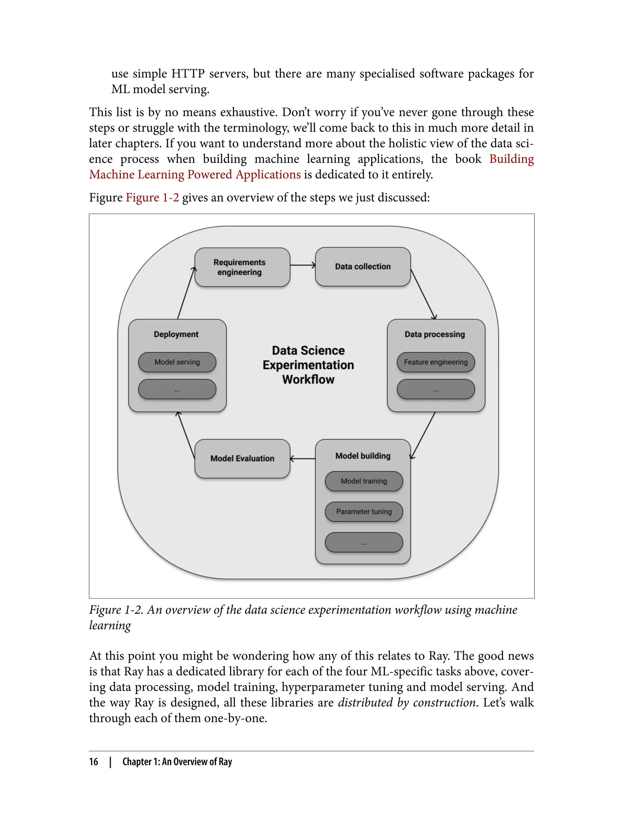
![Data Processing with Ray Data
The first high-level library of Ray we talk about is called “Ray Data”. This library con‐
tains a data structure aptly called Dataset, a multitude of connectors for loading data
from various formats and systems, an API for transforming such datasets, a way to
build data processing pipelines with them, and many integrations with other data
processing frameworks. The Dataset abstraction builds on the powerful Arrow
framework.
To use Ray Data, you need to install Arrow for Python, for instance by running pip
install pyarrow. We’ll now discuss a simple example that creates a distributed Data
set on your local Ray cluster from a Python data structure. Specifically, you’ll create a
dataset from a Python dictionary containing a string name and an integer-valued data
for 10000 entries:
Example 1-2.
import ray
items = [{"name": str(i), "data": i} for i in range(10000)]
ds = ray.data.from_items(items)
ds.show(5)
Creating a Dataset by using from_items from the ray.data module.
Printing the first 10 items of the Dataset.
To show a Dataset means to print some of its values. You should see precisely 5 so-
called ArrowRow elements on your command line, like this:
ArrowRow({'name': '0', 'data': 0})
ArrowRow({'name': '1', 'data': 1})
ArrowRow({'name': '2', 'data': 2})
ArrowRow({'name': '3', 'data': 3})
ArrowRow({'name': '4', 'data': 4})
Great, now you have some distributed rows, but what can you do with that data? The
Dataset API bets heavily on functional programming, as it is very well suited for data
transformations. Even though Python 3 made a point of hiding some of its functional
programming capabilities, you’re probably familiar with functionality such as map,
filter and others. If not, it’s easy enough to pick up. map takes each element of your
dataset and transforms is into something else, in parallel. filter removes data points
according to a boolean filter function. And the slightly more elaborate flat_map first
maps values similarly to map, but then also “flattens” the result. For instance, if map
would produce a list of lists, flat_map would flatten out the nested lists and give you
A Suite of Data Science Libraries | 17](https://image.slidesharecdn.com/76020-250326110013-fba55187/75/Learning-Ray-5th-Early-Release-Max-Pumperla-19-2048.jpg)
![just a list. Equipped with these three functional API calls, let’s see how easily you can
transform your dataset ds:
Example 1-3. Transforming a Dataset with common functional programming routines
squares = ds.map(lambda x: x["data"] ** 2)
evens = squares.filter(lambda x: x % 2 == 0)
evens.count()
cubes = evens.flat_map(lambda x: [x, x**3])
sample = cubes.take(10)
print(sample)
We map each row of ds to only keep the square value of its data entry.
Then we filter the squares to only keep even numbers (a total of 5000 ele‐
ments).
We then use flat_map to augment the remaining values with their respective
cubes.
To take a total of 10 values means to leave Ray and return a Python list with
these values that we can print.
The drawback of Dataset transformations is that each step gets executed synchro‐
nously. In example Example 1-3 this is a non-issue, but for complex tasks that e.g.
mix reading files and processing data, you want an execution that can overlap indi‐
vidual tasks. DatasetPipeline does exactly that. Let’s rewrite the last example into a
pipeline.
Example 1-4.
pipe = ds.window()
result = pipe
.map(lambda x: x["data"] ** 2)
.filter(lambda x: x % 2 == 0)
.flat_map(lambda x: [x, x**3])
result.show(10)
You can turn a Dataset into a pipeline by calling .window() on it.
Pipeline steps can be chained to yield the same result as before.
18 | Chapter 1: An Overview of Ray](https://image.slidesharecdn.com/76020-250326110013-fba55187/75/Learning-Ray-5th-Early-Release-Max-Pumperla-20-2048.jpg)


![• You want to run an extremely computationally expensive training function. In
ML it’s not uncommon to run training procedures that take days, if not weeks,
but let’s say you’re dealing with just a couple of minutes.
• As result of training, you compute a so-called objective function. Usually you
either want to maximize your gains or minimize your losses in terms of perfor‐
mance of your experiment.
• The tricky bit is that your training function might depend on certain parameters,
hyperparameters, that influence the value of your objective function.
• You may have a hunch what individual hyperparameters should be, but tuning
them all can be difficult. Even if you can restrict these parameters to a sensible
range, it’s usually prohibitive to test a wide range of combinations. Your training
function is simply too expensive.
What can you do to efficiently sample hyperparameters and get “good enough” results
on your objective? The field concerned with solving this problem is called hyperpara‐
meter optimization (HPO), and Ray Tune has an enormous suite of algorithms for
tackling it. Let’s look at a first example of Ray Tune used for the situation we just
explained. The focus is yet again on Ray and its API, and not on a specific ML task
(which we simply simulate for now).
Example 1-7. Minimizing an objective for an expensive training function with Ray Tune
from ray import tune
import math
import time
def training_function(config):
x, y = config["x"], config["y"]
time.sleep(10)
score = objective(x, y)
tune.report(score=score)
def objective(x, y):
return math.sqrt((x**2 + y**2)/2)
result = tune.run(
training_function,
config={
"x": tune.grid_search([-1, -.5, 0, .5, 1]),
"y": tune.grid_search([-1, -.5, 0, .5, 1])
})
print(result.get_best_config(metric="score", mode="min"))
A Suite of Data Science Libraries | 23](https://image.slidesharecdn.com/76020-250326110013-fba55187/75/Learning-Ray-5th-Early-Release-Max-Pumperla-25-2048.jpg)
![Serving such a model is a good way to make it accessible. You may not now how to
load and run a TensorFlow model on your computer, but you do now how to ask a
question in plain English. Model serving hides the implementation details of a solu‐
tion and lets users focus on providing inputs and understanding outputs of a model.
To proceed, make sure to run pip install transformers to install the Hugging Face
library that has the model we want to use. With that we can now import and start an
instance of Ray’s serve library, load and deploy a GPT-2 model and ask it for the
meaning of life, like so:
Example 1-8.
from ray import serve
from transformers import pipeline
import requests
serve.start()
@serve.deployment
def model(request):
language_model = pipeline("text-generation", model="gpt2")
query = request.query_params["query"]
return language_model(query, max_length=100)
model.deploy()
query = "What's the meaning of life?"
response = requests.get(f"http://localhost:8000/model?query={query}")
print(response.text)
We start serve locally.
The @serve.deployment decorator turns a function with a request parameter
into a serve deployment.
Loading language_model inside the model function for every request is ineffi‐
cient, but it’s the quickest way to show you a deployment.
We ask the model to give us at most 100 characters to continue our query.
Then we formally deploy the model so that it can start receiving requests over
HTTP.
We use the indispensable requests library to get a response for any question you
might have.
A Suite of Data Science Libraries | 25](https://image.slidesharecdn.com/76020-250326110013-fba55187/75/Learning-Ray-5th-Early-Release-Max-Pumperla-27-2048.jpg)
![7 Spark has been created by another lab in Berkeley, AMPLab. The internet is full of blog posts claiming that
Ray should therefore be seen as a replacement of Spark. It’s better to think of them as tools with different
strengths that are both likely here to stay.
In ??? you will learn how to properly deploy models in various scenarios, but for now
I encourage you to play around with this example and test different queries. Running
the last two lines of code repeatedly will give you different answers practically every
time. Here’s a darkly poetic gem, raising more questions, that I queried on my
machine and slightly censored for underaged readers:
[{
"generated_text": "What's the meaning of life?nn
Is there one way or another of living?nn
How does it feel to be trapped in a relationship?nn
How can it be changed before it's too late?
What did we call it in our time?nn
Where do we fit within this world and what are we going to live for?nn
My life as a person has been shaped by the love I've received from others."
}]
This concludes our whirlwind tour of Ray’s data science libraries, the second of Ray’s
layers. Before we wrap up this chapter, let’s have a very brief look at the third layer,
the growing ecosystem around Ray.
A Growing Ecosystem
Ray’s high-level libraries are powerful and deserve a much deeper treatment through‐
out the book. While their usefulness for the data science experimentation lifecycle is
undeniable, I also don’t want to give off the impression that Ray is all you need from
now on. In fact, I believe the best and most successful frameworks are the ones that
integrate well with existing solutions and ideas. It’s better to focus on your core
strengths and leverage other tools for what’s missing in your solution. There’s usually
no reason to re-invent the wheel.
How Ray Integrates and Extends
To give you an example for how Ray integrates with other tools, consider that Ray
Data is a relatively new addition to its libraries. If you want to boil it down, and
maybe oversimplify a little, Ray is a compute-first framework. In contrast, distributed
frameworks like Apache Spark7
or Dask can be considered data-first. Pretty much
anything you do with Spark starts with the definition of a distributed dataset and
transformations thereof. Dask bets on bringing common data structures like Pandas
dataframes or Numpy arrays to a distributed setup. Both are immensely powerful in
their own regard, and we’ll give you a more detailed and fair comparison to Ray
26 | Chapter 1: An Overview of Ray](https://image.slidesharecdn.com/76020-250326110013-fba55187/75/Learning-Ray-5th-Early-Release-Max-Pumperla-28-2048.jpg)

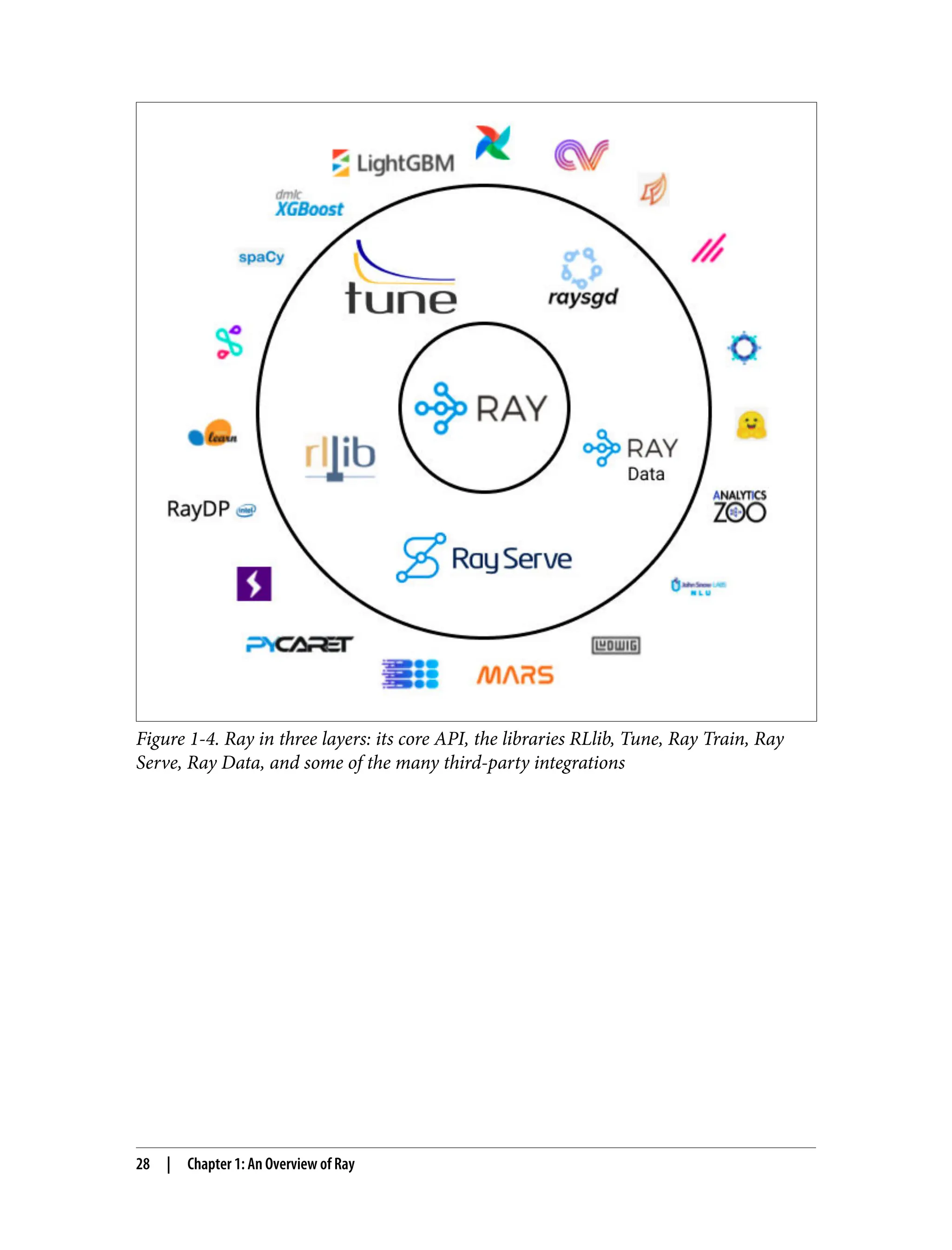
![we’ll do. As before, you can follow this example by typing the code yourself (which is
highly recommended), or by following the notebook for this chapter.
In Chapter 1 we’ve introduced you to the very basics of Ray clusters and showed you
how start a local cluster simply by typing
Example 2-1.
import ray
ray.init()
You’ll need a running Ray cluster to run the examples in this chapter, so make sure
you’ve started one before continuing. The goal of this section is to give you a quick
introduction to the Ray Core API, which we’ll simply refer to as the Ray API from
now on.
As a Python programmer, the great thing about the Ray API is that it hits so close to
home. It uses familiar concepts such as decorators, functions and classes to provide
you with a fast learning experience. The Ray API aims to provide a universal pro‐
gramming interface for distributed computing. That’s certainly no easy feat, but I
think Ray succeeds in this respect, as it provides you with good abstractions that are
intuitive to learn and use. Ray’s engine does all the heavy lifting for you in the back‐
ground. This design philosophy is what enables Ray to be used with existing Python
libraries and systems.
A First Example Using the Ray API
To give you an example, take the following function which retrieves and processes
data from a database. Our dummy database is a plain Python list containing the
words of the title of this book. We act as if retrieving an individual item from this
database and further processing it is expensive by letting Python sleep.
Example 2-2.
import time
database = [
"Learning", "Ray",
"Flexible", "Distributed", "Python", "for", "Data", "Science"
]
def retrieve(item):
time.sleep(item / 10.)
return item, database[item]
30 | Chapter 2: Getting Started With Ray Core](https://image.slidesharecdn.com/76020-250326110013-fba55187/75/Learning-Ray-5th-Early-Release-Max-Pumperla-32-2048.jpg)
![A dummy database containing string data with the title of this book.
We emulate a data-crunching operation that takes a long time.
Our database has eight items, from database[0] for “Learning” to database[7] for
“Science”. If we were to retrieve all items sequentially, how long should that take? For
the item with index 5 we wait for half a second (5 / 10.) and so on. In total, we can
expect a runtime of around (0+1+2+3+4+5+6+7)/10. = 2.8 seconds. Let’s see if that’s
what we actually get:
Example 2-3.
def print_runtime(input_data, start_time, decimals=1):
print(f'Runtime: {time.time() - start_time:.{decimals}f} seconds, data:')
print(*input_data, sep="n")
start = time.time()
data = [retrieve(item) for item in range(8)]
print_runtime(data, start)
We use a list comprehension to retrieve all eight items.
Then we unpack the data to print each item on its own line.
If you run this code, you should see the following output:
Runtime: 2.8 seconds, data:
(0, 'Learning')
(1, 'Ray')
(2, 'Flexible')
(3, 'Distributed')
(4, 'Python')
(5, 'for')
(6, 'Data')
(7, 'Science')
We cut off the output of the program after one decimal number. There’s a little over‐
head that brings the total closer to 2.82 seconds. On your end this might be slightly
less, or much more, depending on your computer. The important take-away is that
our naive Python implementation is not able to run this function in parallel. This
may not come as a surprise to you, but you could have at least suspected that Python
list comprehensions are more efficient in that regard. The runtime we got is pretty
much the worst case scenario, namely the 2.8 seconds we calculated prior to running
the code. If you think about it, it might even be a bit frustrating to see that a program
that essentially sleeps most of its runtime is that slow overall. Ultimately you can
blame the Global Interpreter Lock (GIL) for that, but it gets enough of it already.
An Introduction To Ray Core | 31](https://image.slidesharecdn.com/76020-250326110013-fba55187/75/Learning-Ray-5th-Early-Release-Max-Pumperla-33-2048.jpg)
![2 This example has been adapted from Dean Wampler’s fantastic report “What is Ray?”.
In this way, the function retrieve_task becomes a so-called Ray task. That’s an
extremely convenient design choice, as you can focus on your Python code first, and
don’t have to completely change your mindset or programming paradigm to use Ray.
Note that in practice you would have simply added the @ray.remote decorator to
your original retrieve function (after all, that’s the intended use of decorators), but
we didn’t want to touch previous code to keep things as clear as possible.
Easy enough, so what do you have to change in the code that retrieves the data and
measures performance? It turns out, not much. Let’s have a look at how you’d do that:
Example 2-5. Measuring performance of your Ray task.
start = time.time()
data_references = [retrieve_task.remote(item) for item in range(8)]
data = ray.get(data_references)
print_runtime(data, start, 2)
To run retrieve_task on your local Ray cluster, you use .remote() and pass in
your data as before. You’ll get a list of object references.
To get back data, and not just Ray object references, you use ray.get.
Did you spot the differences? You have to execute your Ray task remotely using the
remote function. When tasks get executed remotely, even on your local cluster, Ray
does so asynchronously. The list items in data_references in the last code snippet do
not contain the results directly. In fact, if you check the Python type of the first item
with type(data_references[0]) you’ll see that it’s in fact an ObjectRef. These
object references correspond to futures which you need to ask the result of. This is
what the call to ray.get(...) is for.
We still want to work more on this example2
, but let’s take a step back here and recap
what we did so far. You started with a Python function and decorated it with
@ray.remote. This made your function a Ray task. Then, instead of calling the origi‐
nal function in your code straight-up, you called .remote(...) on the Ray task. The
last step was to .get(...) the results back from your Ray cluster. I think this proce‐
dure is so intuitive that I’d bet you could already create your own Ray task from
another function without having to look back at this example. Why don’t you give it a
try right now?
Coming back to our example, by using Ray tasks, what did we gain in terms of per‐
formance? On my machine the runtime clocks in at 0.71 seconds, which is just
An Introduction To Ray Core | 33](https://image.slidesharecdn.com/76020-250326110013-fba55187/75/Learning-Ray-5th-Early-Release-Max-Pumperla-35-2048.jpg)
![slightly more than the longest subtask, which comes in at 0.7 seconds. That’s great
and much better than before, but we can further improve our program by leveraging
more of Ray’s API.
Using the object store with put and get
One thing you might have noticed is that in the definition of retrieve we directly
accessed items from our database. Working on a local Ray cluster this is fine, but
imagine you’re running on an actual cluster comprising several computers. How
would all those computers access the same data? Remember from Chapter 1 that in a
Ray cluster there is one head node with a driver process (running ray.init()) and
many worker nodes with worker processes executing your tasks. My laptop has a total
of 8 CPU cores, so Ray will create 8 worker processes on my one-node local cluster.
Our database is currently defined on the driver only, but the workers running your
tasks need to have access to it to run the retrieve task. Luckily, Ray provides an easy
way to share data between the driver and workers (or between workers). You can sim‐
ply use put to place your data into Ray’s distributed object store and then use get on
the workers to retrieve it as follows.
Example 2-6.
database_object_ref = ray.put(database)
@ray.remote
def retrieve_task(item):
obj_store_data = ray.get(database_object_ref)
time.sleep(item / 10.)
return item, obj_store_data[item]
put your database into the object store and receive a reference to it.
This allows your workers to get the data, no matter where they are located in the
cluster.
By using the object store this way, you can let Ray handle data access across the whole
cluster. We’ll talk about how exactly data is passed between nodes and within workers
when talking about Ray’s infrastructure. While the interaction with the object store
requires some overhead, Ray is really smart about storing the data, which gives you
performance gains when working with larger, more realistic datasets. For now, the
important part is that this step is essential in a truly distributed setting. If you like, try
to re-run Example 2-5 with this new retrieve_task function and confirm that it still
runs, as expected.
34 | Chapter 2: Getting Started With Ray Core](https://image.slidesharecdn.com/76020-250326110013-fba55187/75/Learning-Ray-5th-Early-Release-Max-Pumperla-36-2048.jpg)
![Using Ray’s wait function for non-blocking calls
Note how in Example 2-5 we used ray.get(data_references) to access results. This
call is blocking, which means that our driver has to wait for all the results to be avail‐
able. That’s not a big deal in our case, the program now finishes in under a second.
But imagine processing of each data item would take several minutes. In that case you
would want to free up the driver process for other tasks, instead of sitting idly by.
Also, it would be great to process results as they come in (some finish much quicker
than others), rather than waiting for all data to be processed. One more question to
keep in mind is what happens if one of the data items can’t be retrieved as expected?
Let’s say there’s a deadlock somewhere in the database connection. In that case, the
driver will simply hang and never retrieve all items. For that reason it’s a good idea to
work with reasonable timeouts. In our scenario, we should not wait longer than 10
times the longest data retrieval task before stopping the task. Here’s how you can do
that with Ray by using wait:
Example 2-7.
start = time.time()
data_references = [retrieve_task.remote(item) for item in range(8)]
all_data = []
while len(data_references) > 0:
finished, data_references = ray.wait(data_references, num_returns=2, timeout=7.0)
data = ray.get(finished)
print_runtime(data, start, 3)
all_data.extend(data)
Instead of blocking, we loop through unfinished data_references.
We asynchronously wait for finished data with a reasonable timeout. data_ref
erences gets overridden here, to prevent an infinite loop.
We print results as they come in, namely in blocks of two.
Then we append new data to the all_data until finished.
As you can see ray.wait returns two arguments, namely finished data and futures
that still need to be processed. We use the num_returns argument, which defaults to
1, to let wait return whenever a new pair of data items is available. On my laptop this
results in the following output:
Runtime: 0.108 seconds, data:
(0, 'Learning')
(1, 'Ray')
Runtime: 0.308 seconds, data:
An Introduction To Ray Core | 35](https://image.slidesharecdn.com/76020-250326110013-fba55187/75/Learning-Ray-5th-Early-Release-Max-Pumperla-37-2048.jpg)
![(2, 'Flexible')
(3, 'Distributed')
Runtime: 0.508 seconds, data:
(4, 'Python')
(5, 'for')
Runtime: 0.709 seconds, data:
(6, 'Data')
(7, 'Science')
Note how in the while loop, instead of just printing results, we could have done many
other things, like starting entirely new tasks on other workers with the data already
retrieved up to this point.
Handling task dependencies
So far our example program has been fairly easy on a conceptual level. It consists of a
single step, namely retrieving a bunch of data. Now, imagine that once your data is
loaded you want to run a follow-up processing task on it. To be more concrete, let’s
say we want to use the result of our first retrieve task to query other, related data (pre‐
tend that you’re querying data from a different table in the same database). The fol‐
lowing code sets up such a task and runs both our retrieve_task and
follow_up_task consecutively.
Example 2-8. Running a follow-up task that depends on another Ray task
@ray.remote
def follow_up_task(retrieve_result):
original_item, _ = retrieve_result
follow_up_result = retrieve(original_item + 1)
return retrieve_result, follow_up_result
retrieve_refs = [retrieve_task.remote(item) for item in [0, 2, 4, 6]]
follow_up_refs = [follow_up_task.remote(ref) for ref in retrieve_refs]
result = [print(data) for data in ray.get(follow_up_refs)]
Using the result of retrieve_task we compute another Ray task on top of it.
Leveraging the original_item from the first task, we retrieve more data.
Then we return both the original and the follow-up data.
We pass the object references from the first task into the second task.
Running this code results in the following output.
36 | Chapter 2: Getting Started With Ray Core](https://image.slidesharecdn.com/76020-250326110013-fba55187/75/Learning-Ray-5th-Early-Release-Max-Pumperla-38-2048.jpg)
![3 According to Clarke’s third law any sufficiently advanced technology is indistinguishable from magic. For me,
this example has a bit of magic to it.
((0, 'Learning'), (1, 'Ray'))
((2, 'Flexible'), (3, 'Distributed'))
((4, 'Python'), (5, 'for'))
((6, 'Data'), (7, 'Science'))
If you don’t have a lot of experience with asynchronous programming, you might not
be impressed by Example 2-8. But I hope to convince you that it’s at least a bit sur‐
prising3
that this code snippet runs at all. So, what’s the big deal? After all, the code
reads like regular Python - a function definition and a few list comprehensions. The
point is that the function body of follow_up_task expects a Python tuple for its
input argument retrieve_result, which we unpack in the first line of the function
definition.
But by invoking [follow_up_task.remote(ref) for ref in retrieve_refs] we
do not pass in tuples to the follow-up task at all. Instead, we pass in Ray object refer‐
ences with retrieve_refs. What happens under the hood is that Ray knows that fol
low_up_task requires actual values, so internally in this task it will call ray.get to
resolve the futures. Ray builds a dependency graph for all tasks and executes them in
an order that respects the dependencies. You do not have to tell Ray explicitly when
to wait for a previous task to finish, it will infer that information for you.
The follow-up tasks will only be scheduled, once the individual retrieve tasks have
finished. If you ask me, that’s an incredible feature. In fact, if I had called
retrieve_refs something like retrieve_result, you may not even have noticed this
important detail. That’s by design. Ray wants you to focus on your work, not on the
details of cluster computing. In figure Figure 2-1 you can see the dependency graph
for the two tasks visualized.
An Introduction To Ray Core | 37](https://image.slidesharecdn.com/76020-250326110013-fba55187/75/Learning-Ray-5th-Early-Release-Max-Pumperla-39-2048.jpg)
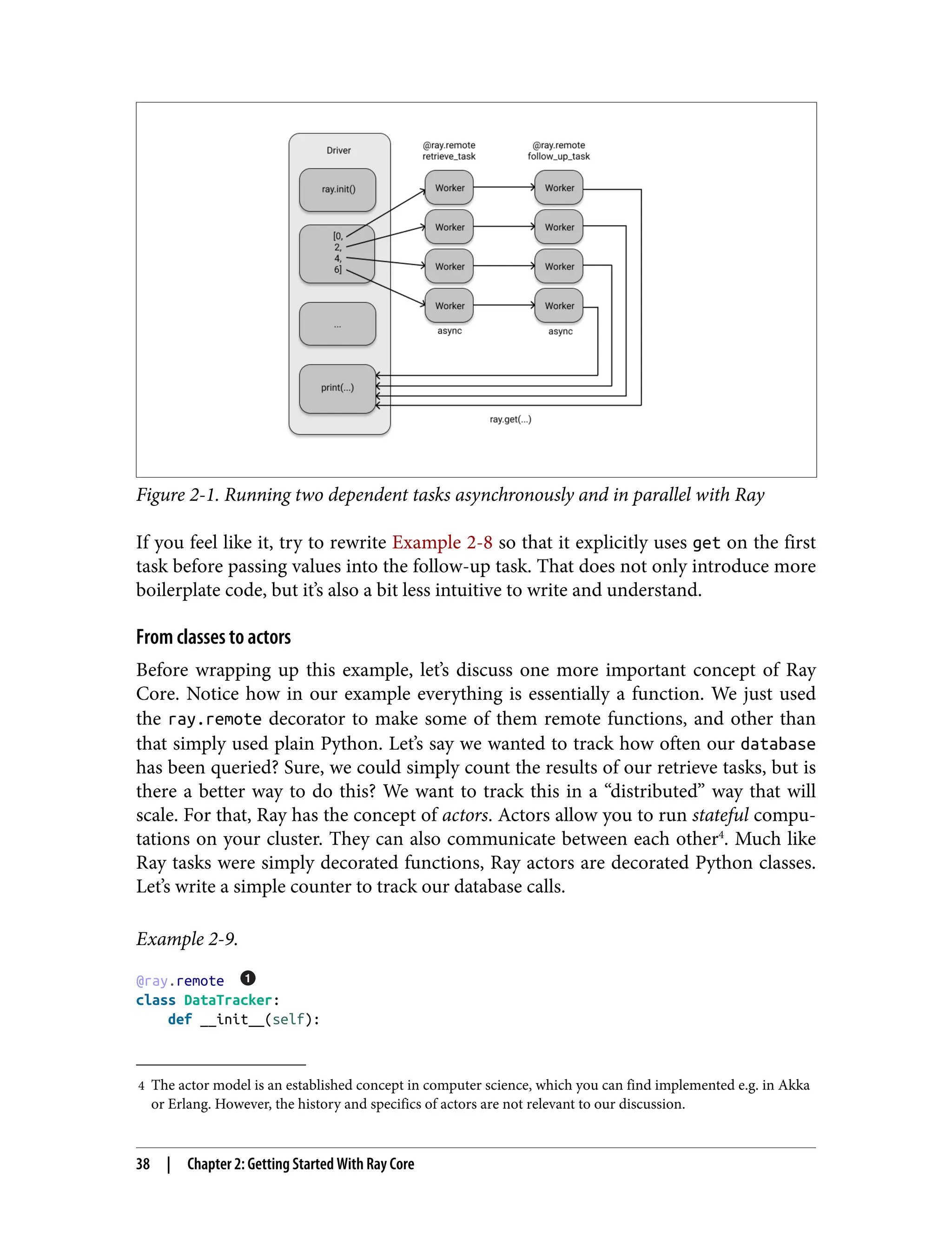
![self._counts = 0
def increment(self):
self._counts += 1
def counts(self):
return self._counts
We can make any Python class a Ray actor by using the same ray.remote decora‐
tor as before.
This DataTracker class is already an actor, since we equipped it with the ray.remote
decorator. This actor can track state, here just a simple counter, and its methods are
Ray tasks that get invoked precisely like we did with functions before, namely
using .remote(). Let’s see how we can modify our existing retrieve_task to incor‐
porate this new actor.
Example 2-10.
@ray.remote
def retrieve_tracker_task(item, tracker):
obj_store_data = ray.get(database_object_ref)
time.sleep(item / 10.)
tracker.increment.remote()
return item, obj_store_data[item]
tracker = DataTracker.remote()
data_references = [retrieve_tracker_task.remote(item, tracker) for item in range(8)]
data = ray.get(data_references)
print(ray.get(tracker.counts.remote()))
We pass in the tracker actor into this task.
The tracker receives an increment for each call.
We instantiate our DataTracker actor by calling .remote() on the class.
The actor gets passed into the retrieve task.
Afterwards we can get the counts state from our tracker from another remote
invocation.
Unsurprisingly, the result of this computation is in fact 8. We didn’t need actors to
compute this, but I hope you can see how useful it can be to have a mechanism to
track state across the cluster, potentially spanning multiple tasks. In fact, we could
An Introduction To Ray Core | 39](https://image.slidesharecdn.com/76020-250326110013-fba55187/75/Learning-Ray-5th-Early-Release-Max-Pumperla-41-2048.jpg)


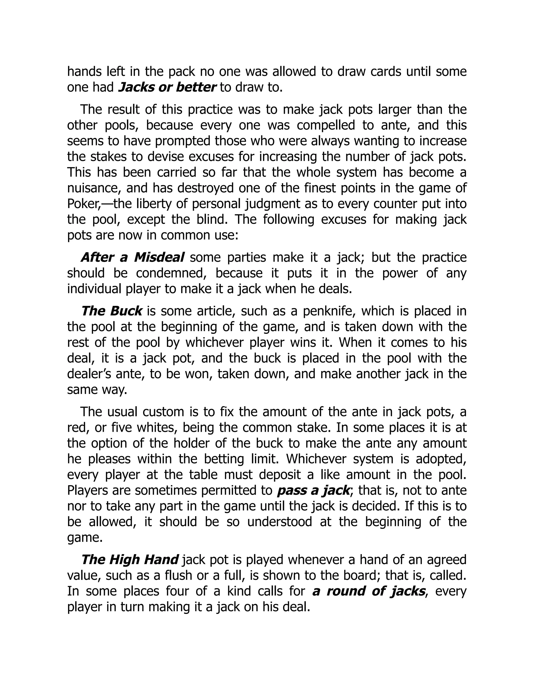

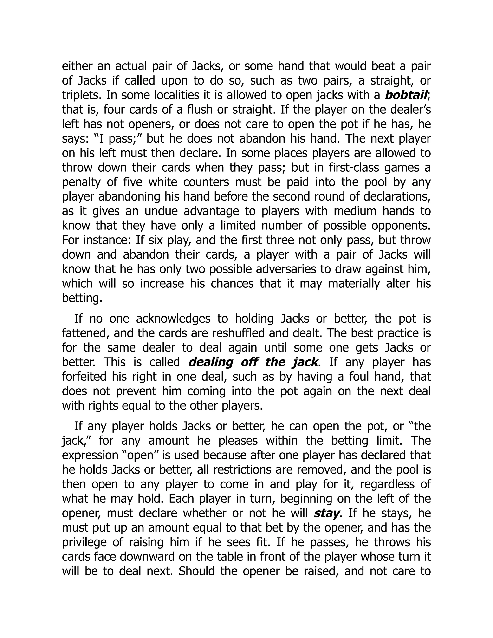

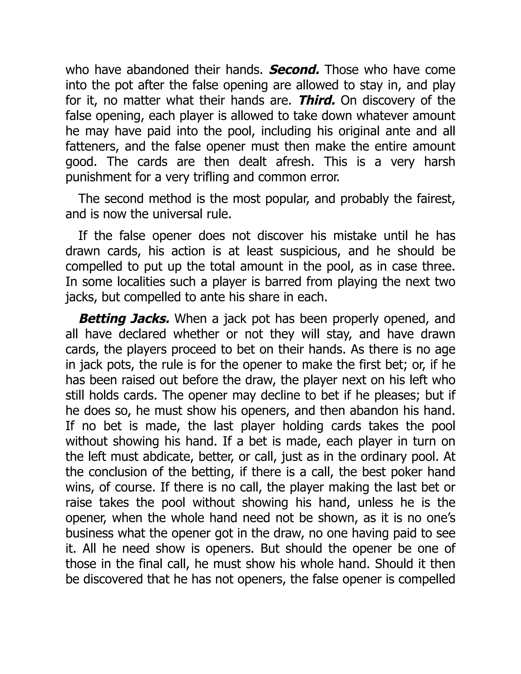
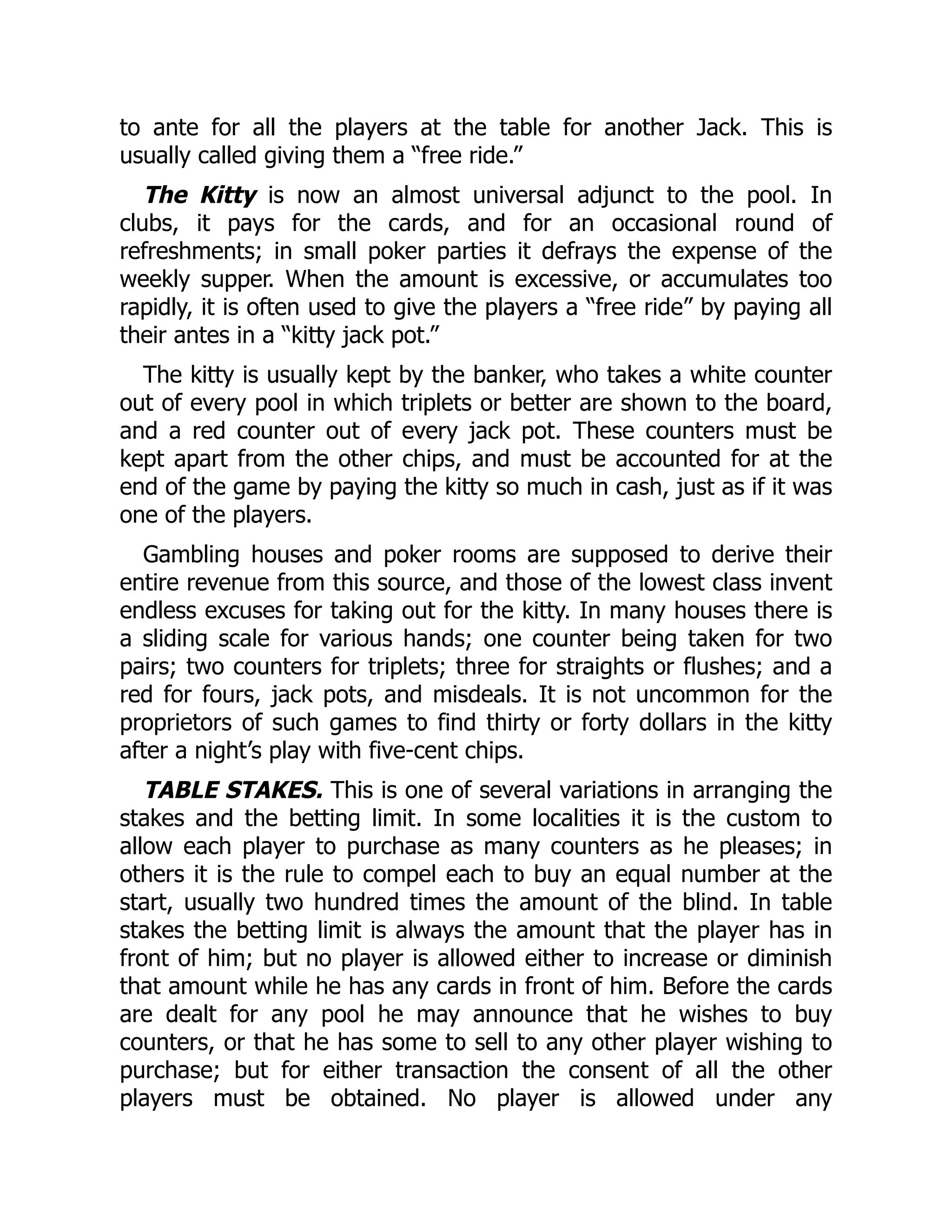


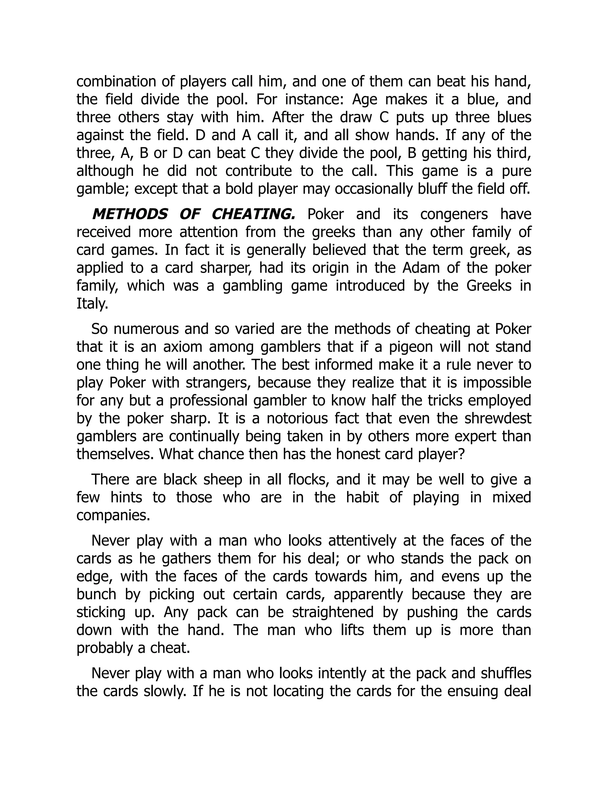

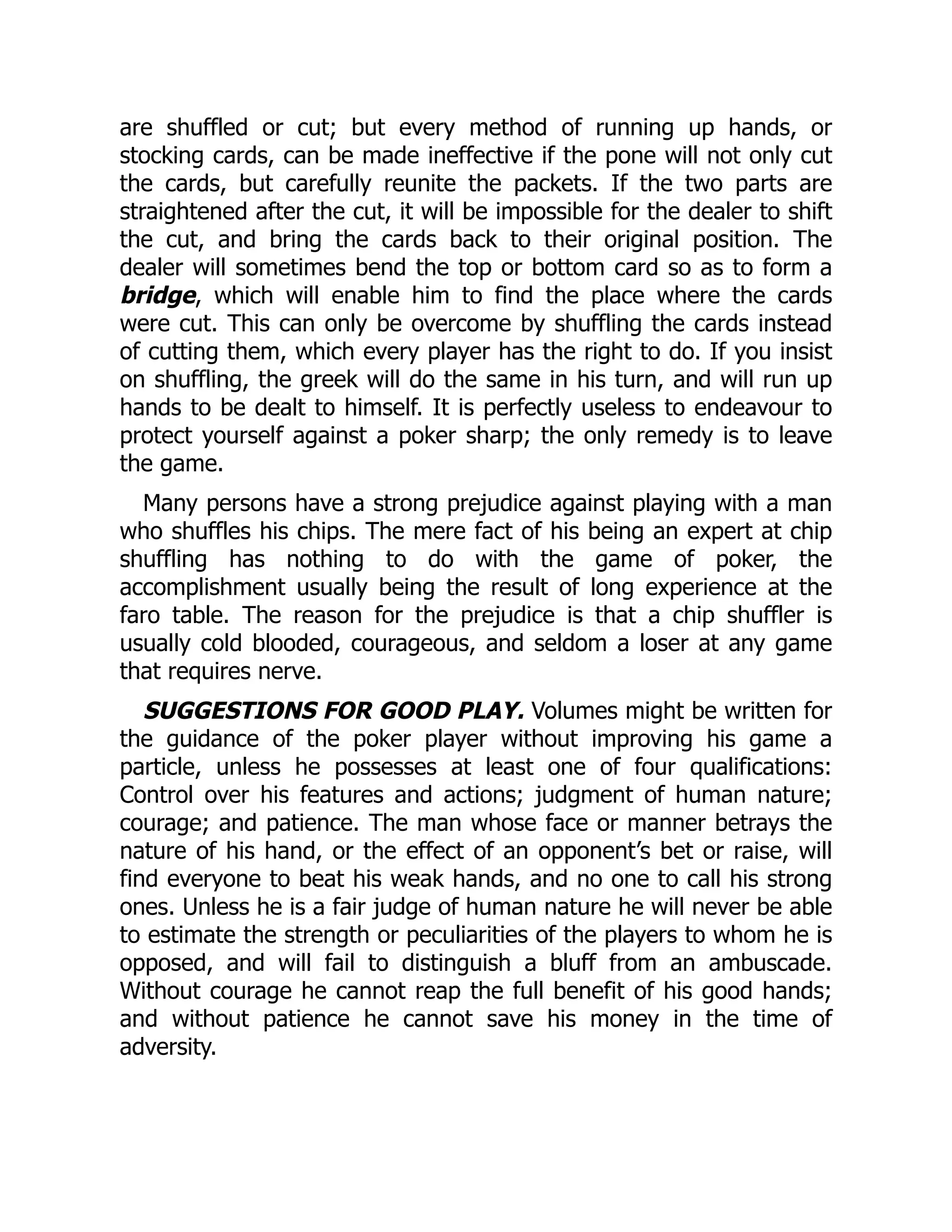

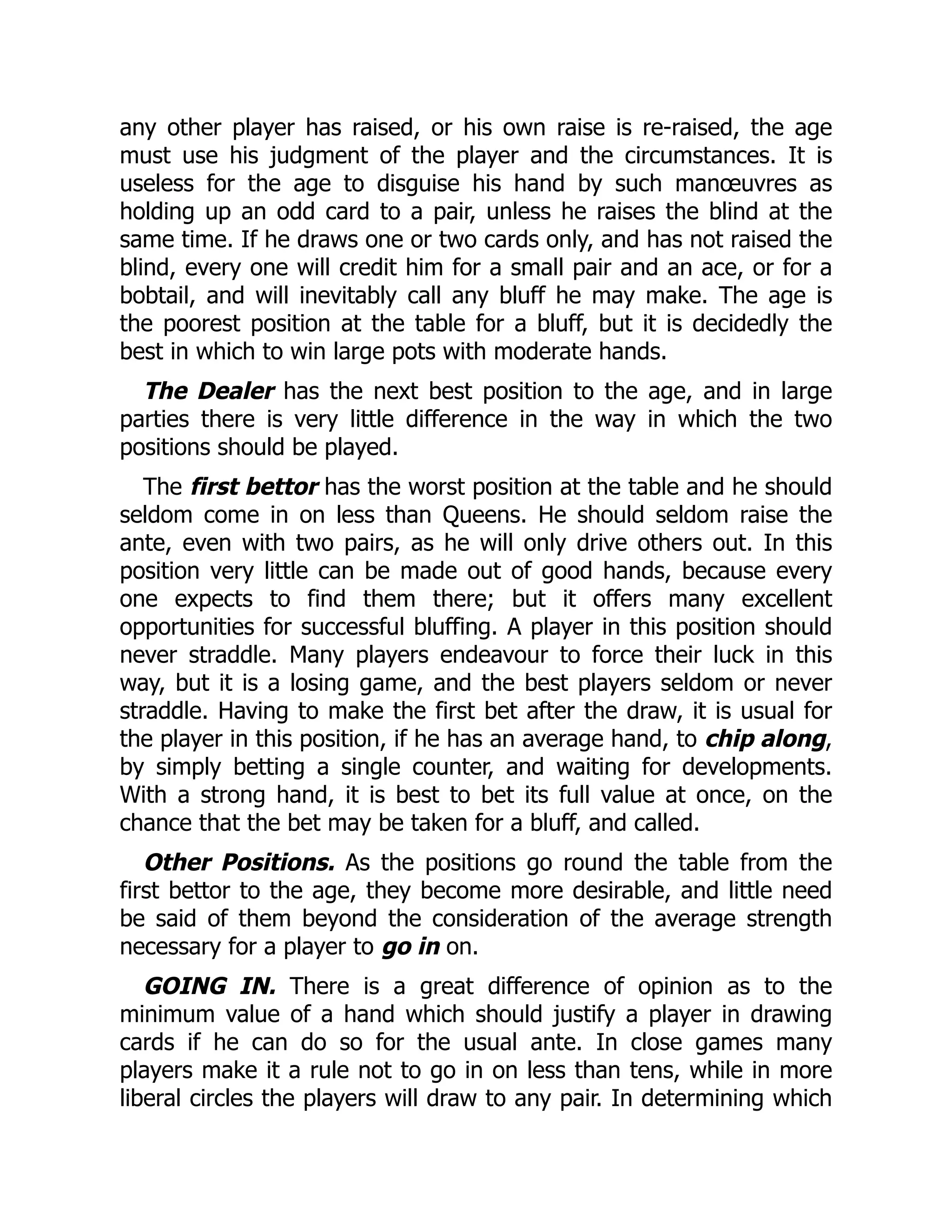
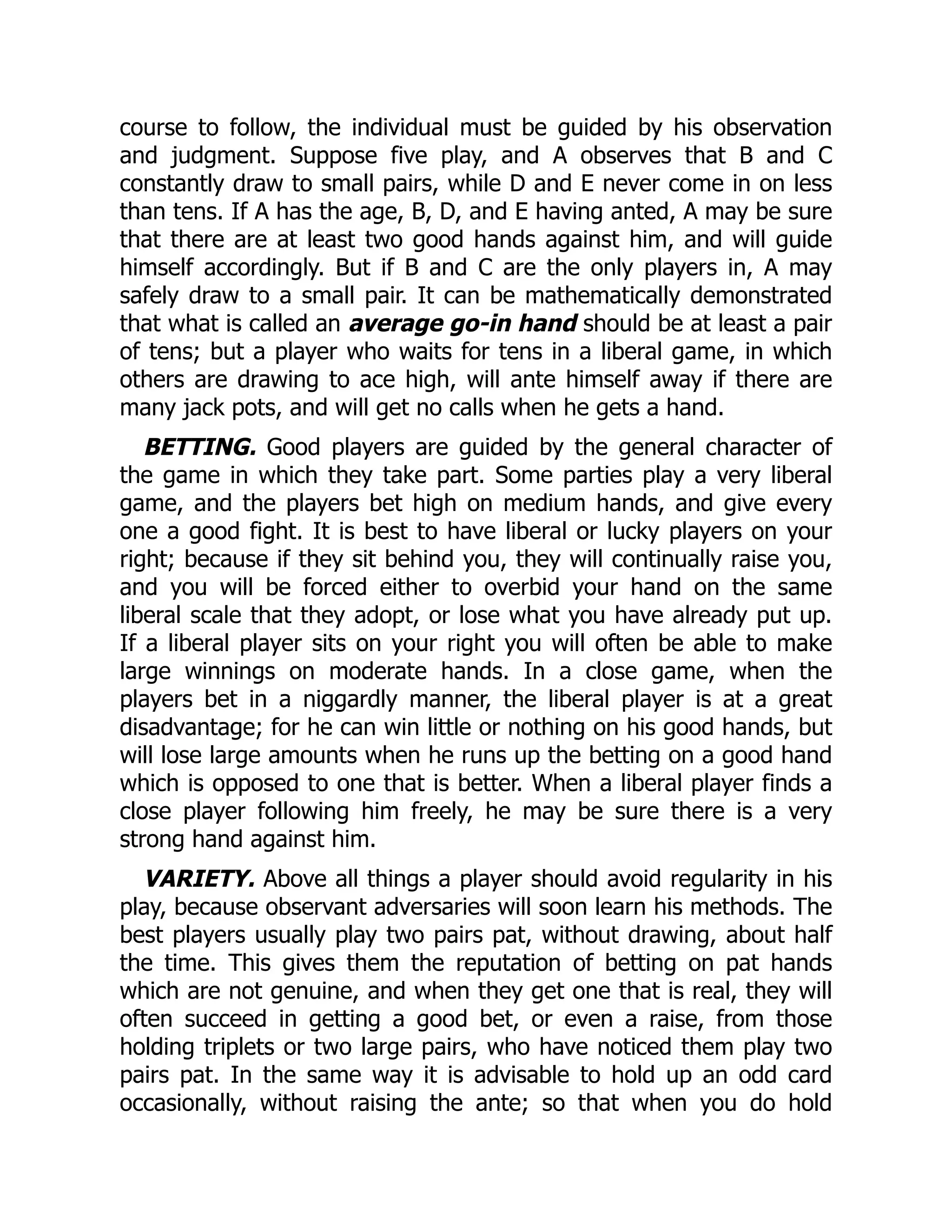

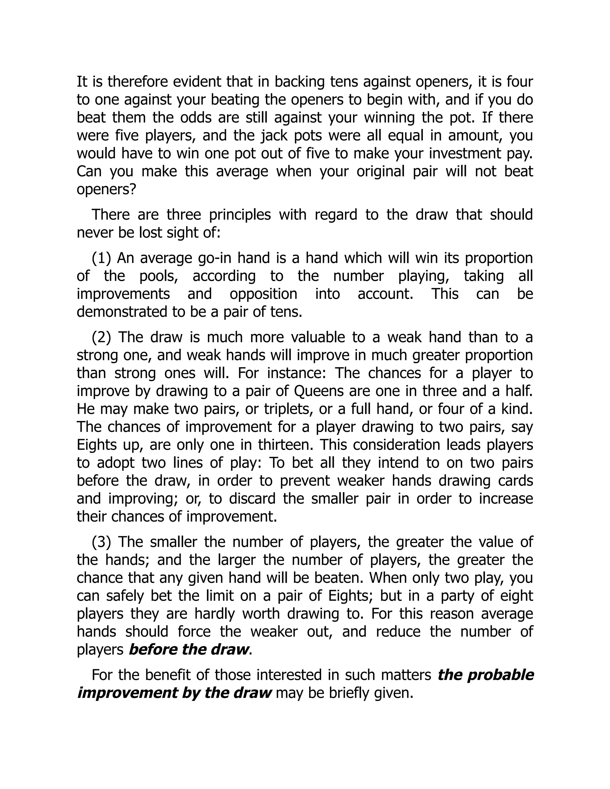


![2. Cutting. The players who shall form the table, and their
positions at the beginning of the game may be decided by drawing
from an outspread pack, or by throwing round a card to each
candidate, face up. If there are eight or more candidates, the tables
shall divide evenly if the number is even, those cutting the highest
cards playing together. If the number is odd, the smaller table shall
be formed by those cutting the highest cards. In cutting, the ace is
low. Any player exposing more than one card must cut again.
3. The table formed, the players draw from the outspread pack for
positions. The lowest cut has the first choice, and deals the first
hand. The player cutting the next lowest has the next choice, and so
on until all are seated.
4. Ties. If players cut cards of equal value they must cut again;
but the new cut decides nothing but the tie.
5. Stakes. Any player may be the banker, and keep the kitty, if
any. In Draw, Straight, or Stud Poker, each player may purchase as
many counters as he pleases. In Freeze-out, Table Stakes, Whiskey
Poker, and Progressive Poker, each player must begin with an equal
amount.
6. Betting Limits. Before play begins limits must be agreed upon
for the amount of the blind, the straddle, the ante in jack pots, and
for betting or raising.
7. Shuffling. Before the first deal the pack must be counted to
see that it contains the proper number of cards. Should the first
dealer neglect this he forfeits five counters to the pool. Before each
deal the cards must be shuffled. Any player may shuffle, the dealer
last.
8. Cutting to the Dealer. The dealer must present the pack to
the pone, [the player on his right,] to be cut. The pone may either
cut, or signify that he does not wish to do so, by tapping the pack
with his knuckles. Should the pone decline to cut, no other player
can insist on his doing so, nor do it for him. If he cuts, he must leave
at least four cards in each packet, and the dealer or the pone must](https://image.slidesharecdn.com/76020-250326110013-fba55187/75/Learning-Ray-5th-Early-Release-Max-Pumperla-65-2048.jpg)
![reunite the packets by placing the one not removed in cutting upon
the other.
9. If in cutting, or in reuniting the packets, a card is exposed, the
pack must be reshuffled and cut.
10. If the dealer reshuffles the pack after it has been properly cut,
he forfeits five counters to the current pool.
11. Dealing Before the Draw. After the age, [the player on the
dealer’s left,] has put up the amount of the blind, the dealer
distributes the cards face down, one at a time, in rotation, until each
player has received five cards.
12. The deal passes to the left, except in jack pots, when it may
be agreed that the same dealer shall deal until the pot is opened.
13. Misdealing. A misdeal does not lose the deal; the same
dealer must deal again. It is a misdeal: If the dealer fails to present
the pack to the pone; or if any card is found faced in the pack; or if
the pack is found imperfect; or if the dealer gives six or more cards
to more than one player; or if he deals more or fewer hands than
there are players; or if he omits a player in dealing; or if he deals a
card incorrectly, and fails to correct the error before dealing another.
14. Irregularities in the Hands. Should the dealer, or the wind,
turn over any card, the player to whom it is dealt must take it; but
the same player cannot be compelled to take two exposed cards.
Should such a combination occur there must be a new deal. If the
player exposes cards himself, he has no remedy.
15. Should any player receive more or less than his proper
number of cards, and discover the error before he looks at any card
in his hand, or lifts it from the table, he may demand a new deal if
no bet has been made; or he may ask the dealer to give him another
card from the pack if he has too few, or to draw a card if he has too
many. Cards so drawn must not be exposed, but should be placed
on the top of the pack. If a bet has been made, there must be a
new deal. Should the player take up his hand, or look at any card in
it, he has no remedy.](https://image.slidesharecdn.com/76020-250326110013-fba55187/75/Learning-Ray-5th-Early-Release-Max-Pumperla-66-2048.jpg)