Download as PDF, PPTX
![Location Graph
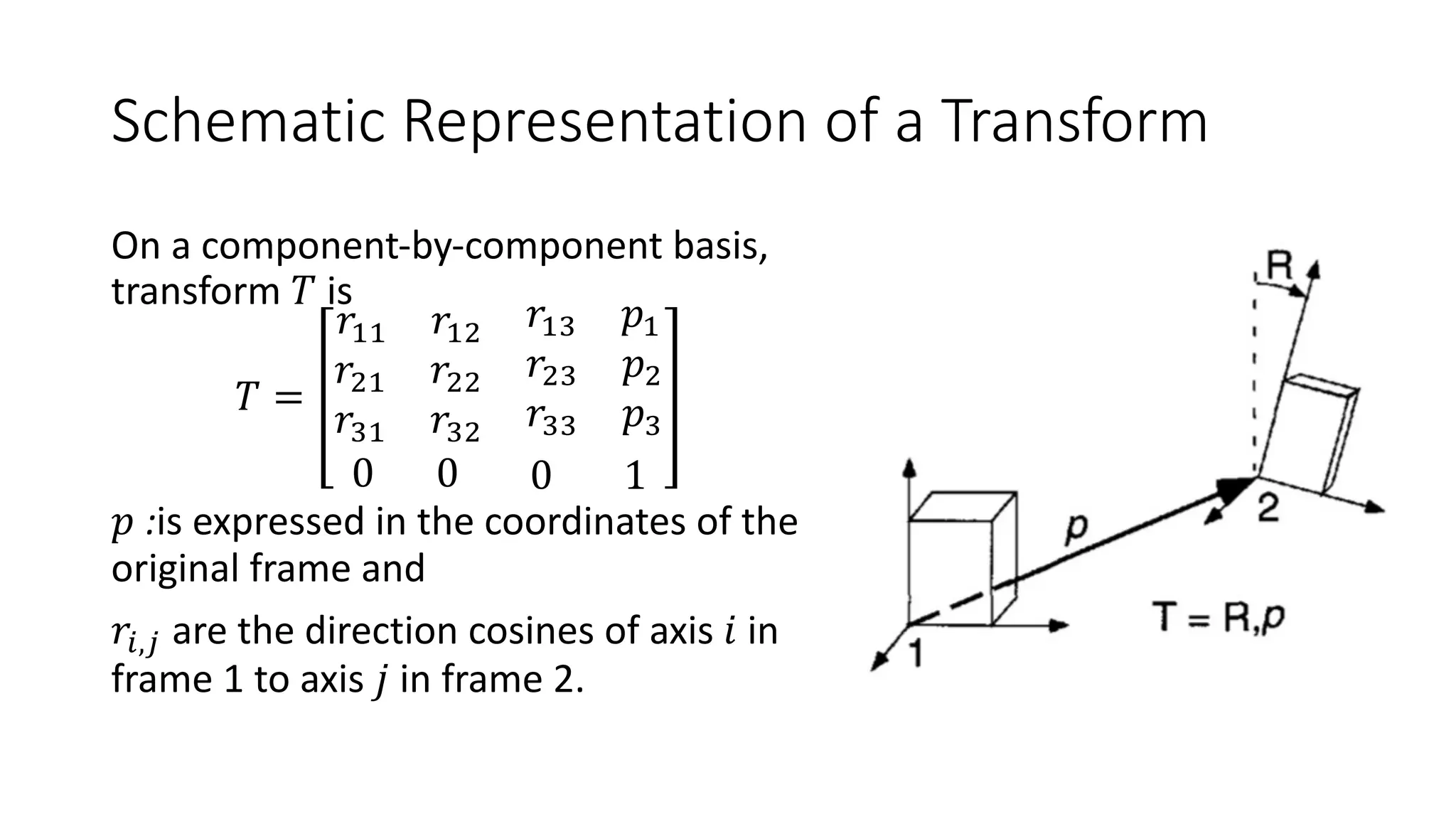
Coordinate system is the means used to specify location of one part
relative to other.
A chain of locations can be defined such that each location is defined in
terms of [T] another part’s coordinate system.
A set of these chains results in a location graph. Part to part is related
by the transformation matrix [T].](https://image.slidesharecdn.com/lecture-8b-assembly-modeling-240327125046-686ff18a/75/Leacture-about-assembly-modeling-pdf-60-2048.jpg)
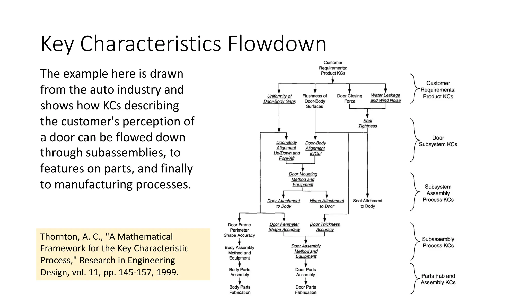
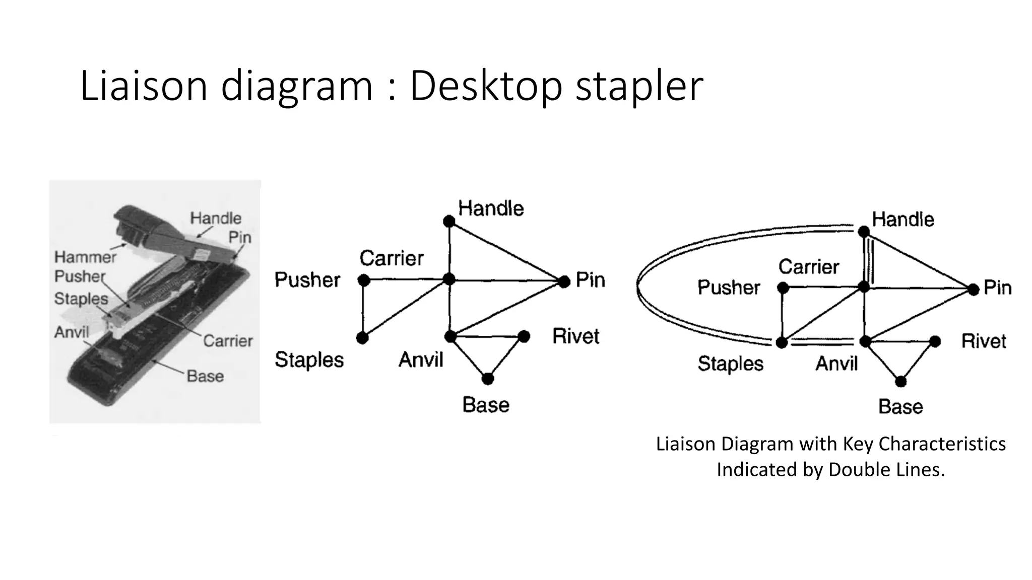
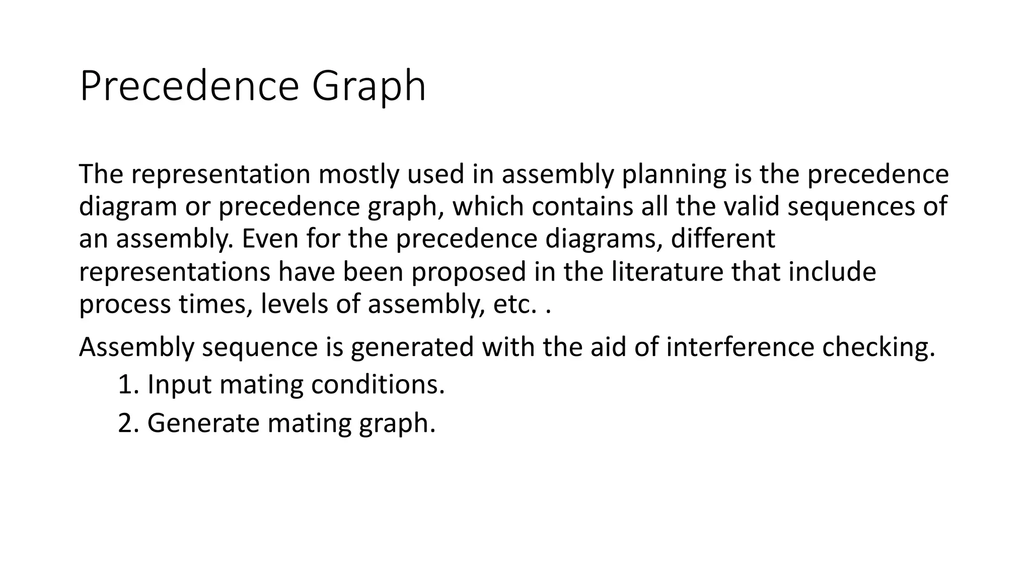
![Key characteristics
Key characteristics are the product, subassembly, part, and process
features whose variation from nominal significantly impacts the final
cost, performance [including the customer's perception of quality], or
safety of a product. Special control should be applied to those KCs if the
cost of variation justifies the cost of control.
Thornton, A. C., "A Mathematical Framework for the Key Characteristic Process,"
Research in Engineering Design, vol. 11, pp. 145-157, 1999.](https://image.slidesharecdn.com/lecture-8b-assembly-modeling-240327125046-686ff18a/75/Leacture-about-assembly-modeling-pdf-75-2048.jpg)

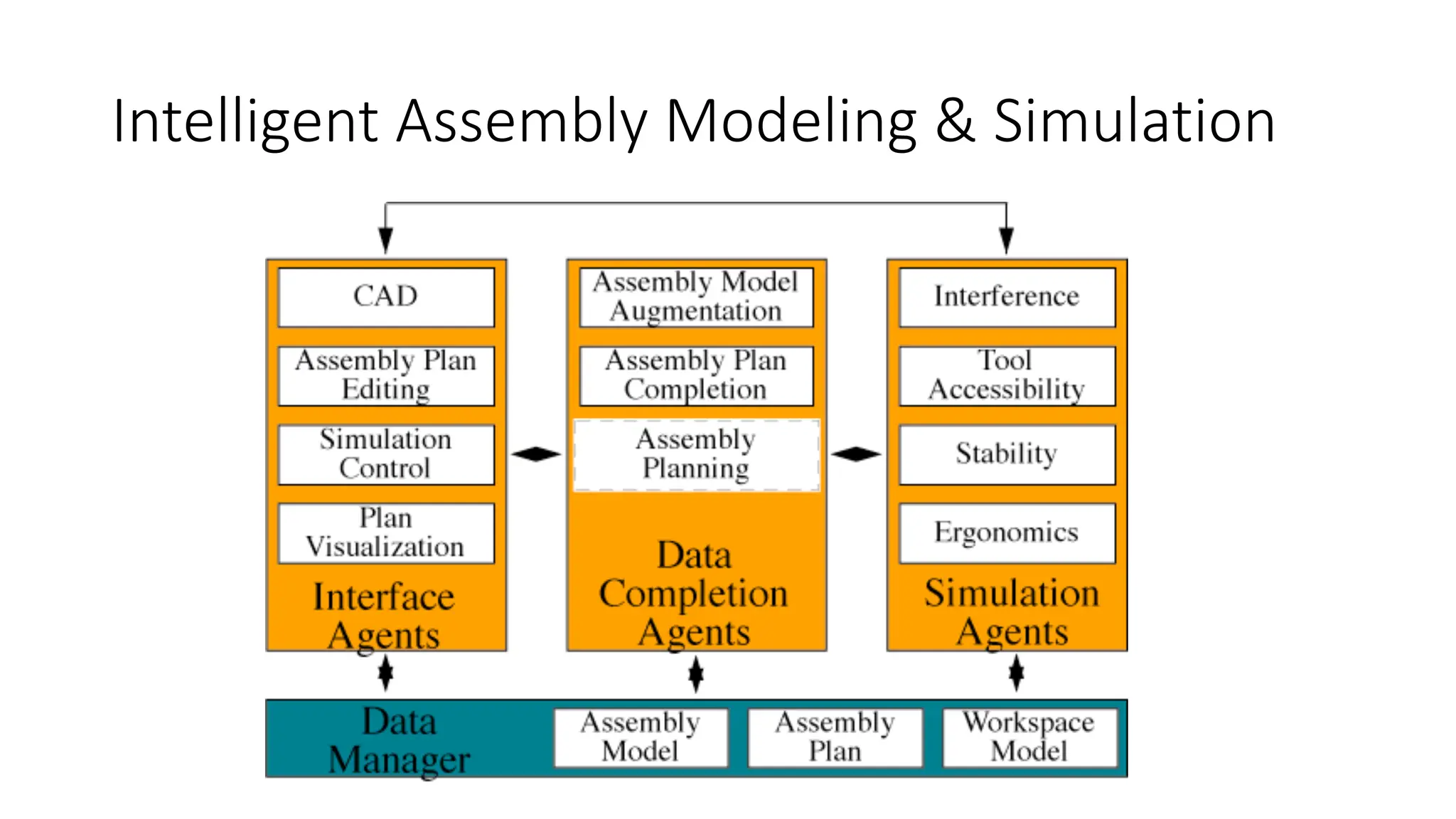
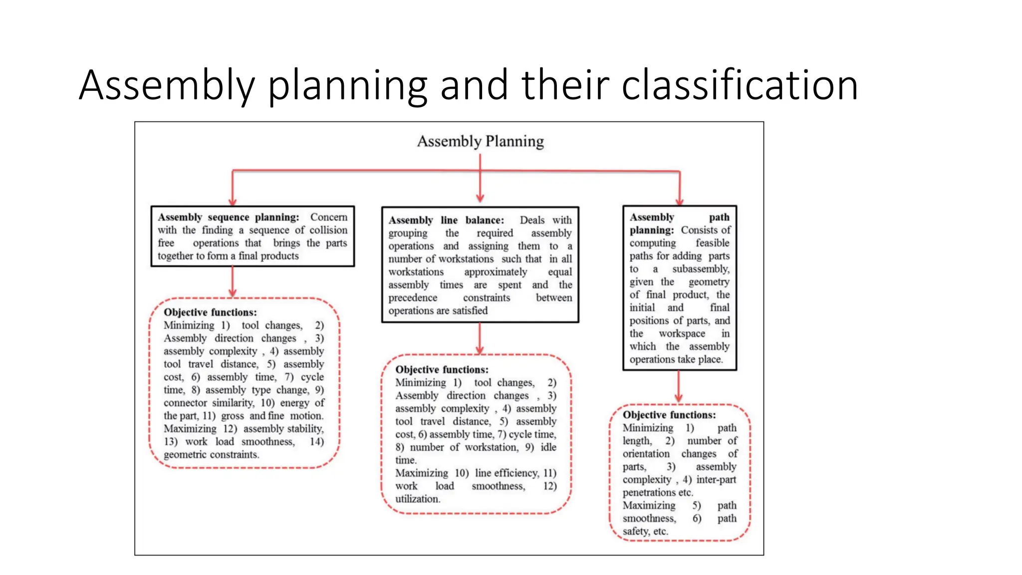

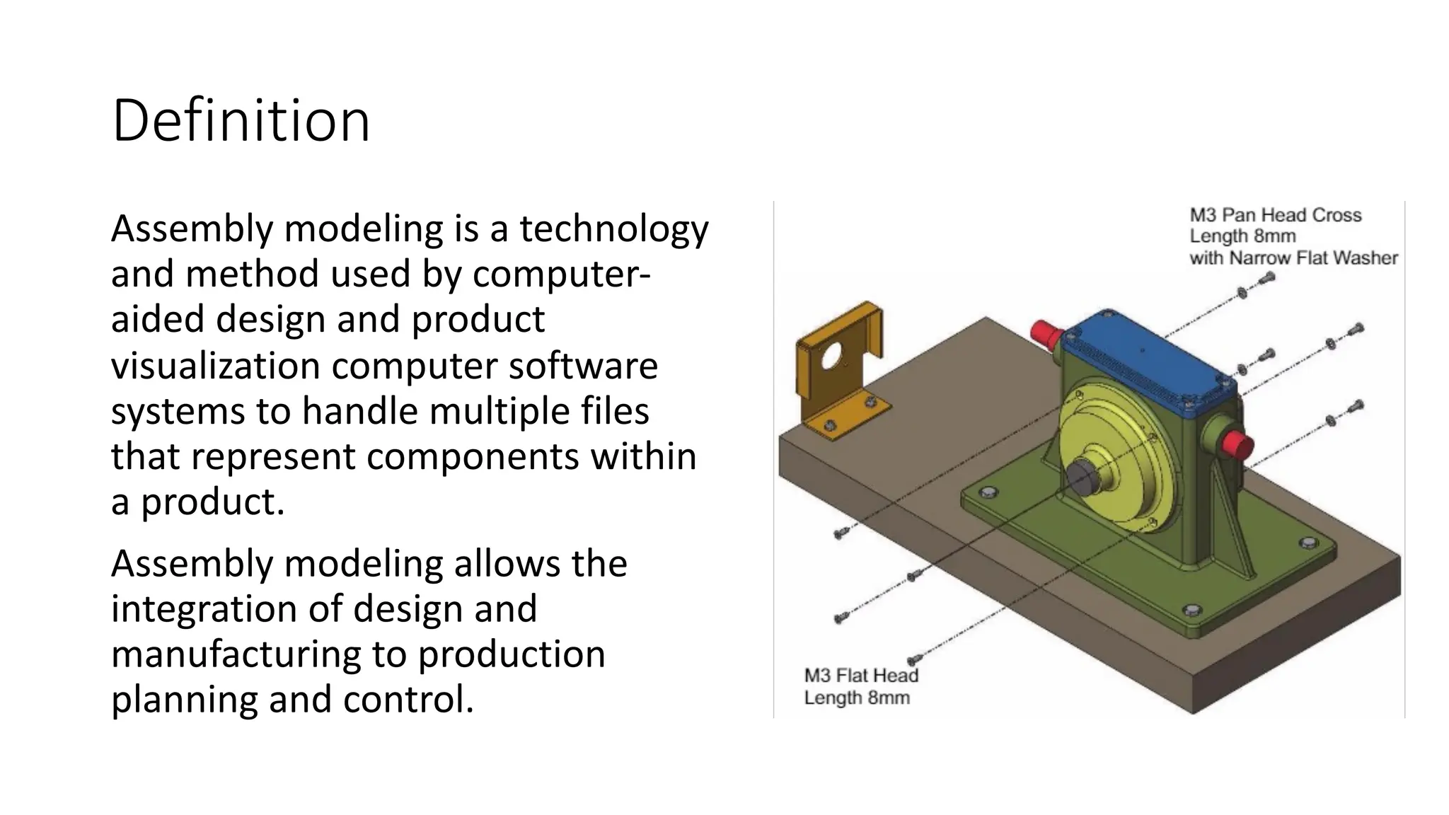
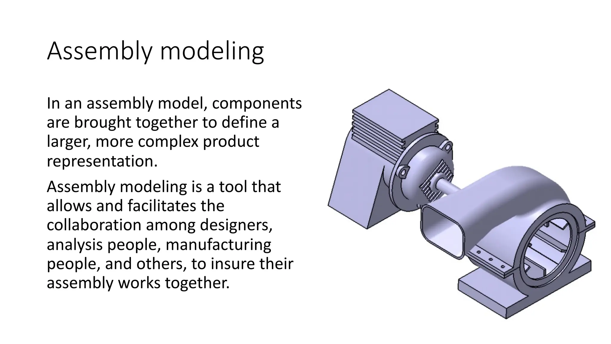
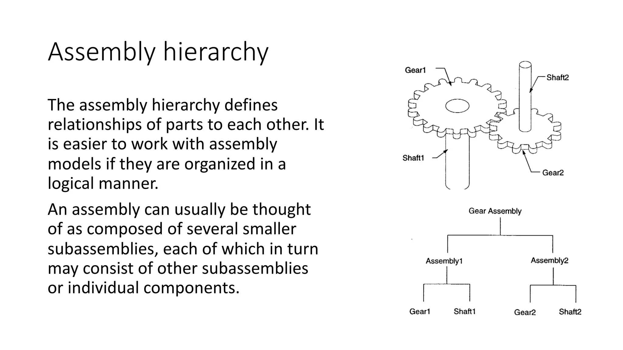
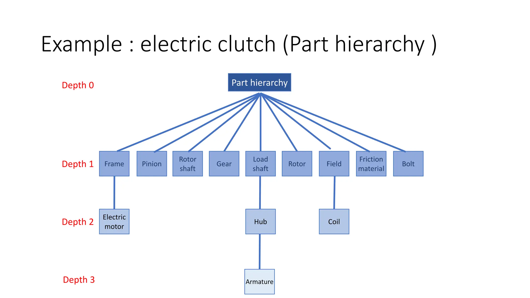
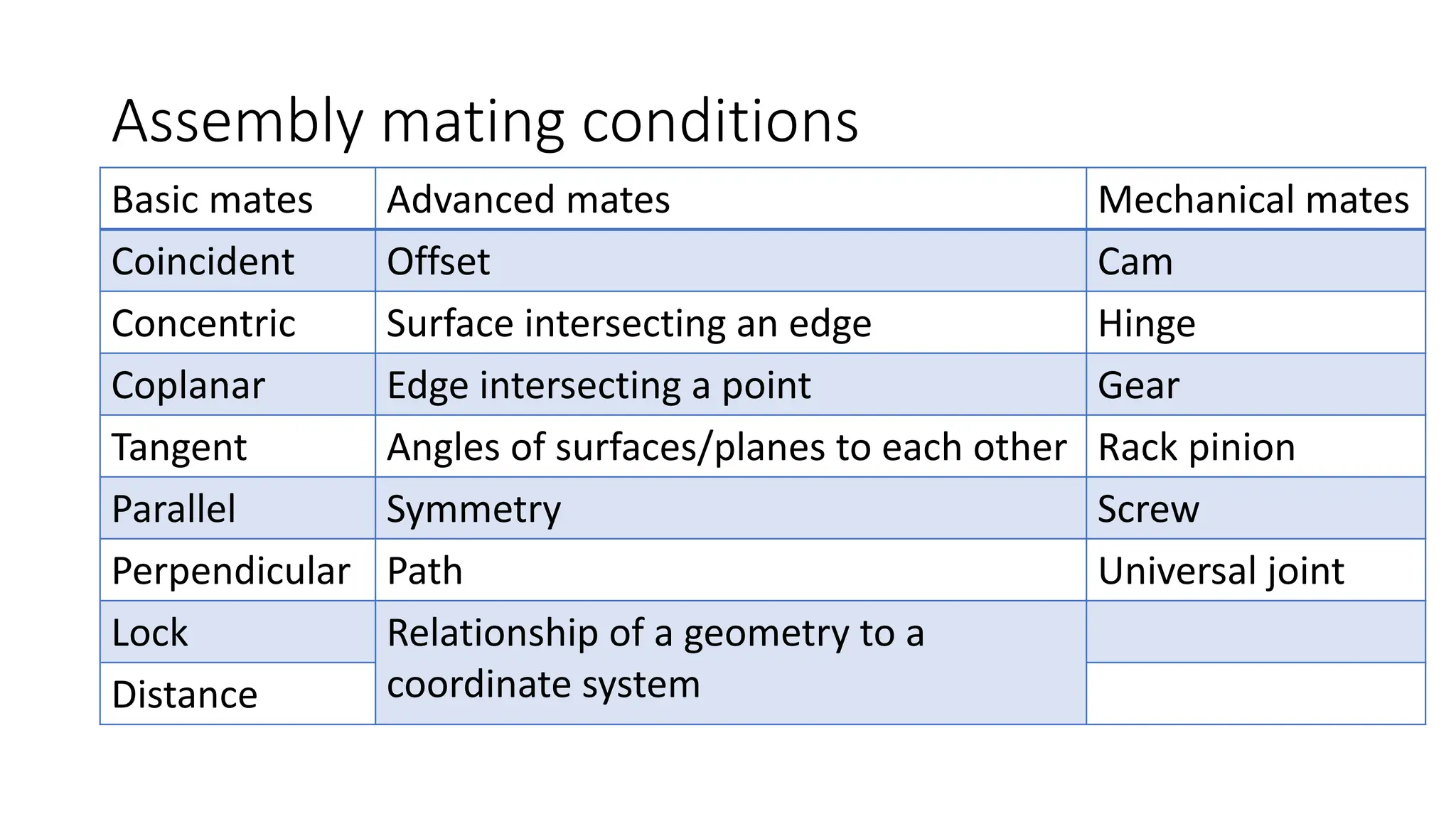
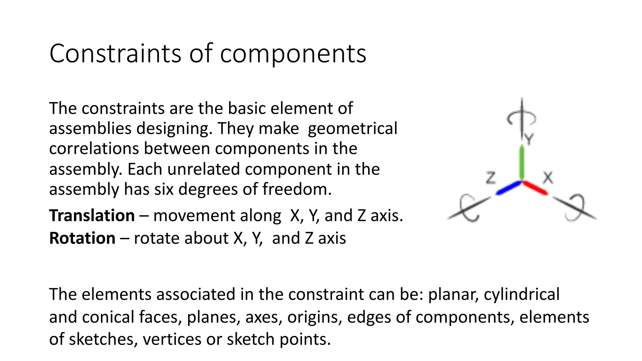
Assembly modeling involves bringing together component models to define larger, more complex product representations in a hierarchical structure. Components are constrained together using various mating conditions like concentric, coincident, parallel etc. Assembly models can be constructed using bottom-up, top-down or mixed approaches and represented using graph structures that show relationships between parts. Assembly modeling facilitates collaboration across design, analysis, manufacturing and other functions.