This document contains solutions to tutorial problems for a thermodynamics and heat transfer textbook. It includes 9 problems solved relating to concepts like heat transfer processes, Fourier's law, heat loss through windows, convection coefficients, and the Stefan-Boltzmann law. The problems calculate values like heat loss rates, temperature differences, convection coefficients, and maximum allowable chip powers using equations of heat transfer.

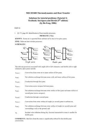
1. MECH3400 Thermodynamics and Heat Transfer
Solutions for tutorial problems (Tutorial 1)
Textbook: Incropera and Dewitt (5th edition)
(by Bo Feng, 2006)
PART II
1. Q1.73, page 48. Identification of heat transfer processes.

5. 2. Q1.5, page 34. The inner and outer surface temperatures of a glass window 5 mm thick are 15
and 5 °C. What is the heat loss through a window that is 1m by 3 m on a side? The thermal
conductivity of glass is 1.4 W/mK.
Solution:
Assume the process is at steady state and the direction of x is from the inner surface to the
outer surface. The heat loss may be obtained from Fourier’s law:
ΔT (5 − 15) K
q = −kA = −1.4W / mK × (1m × 3m ) = 8.4kW
L 5 × 10 −3 m
The value is positive, indicating the direction of heat flow is from the inner surface to the
outer surface.
3. Q1.6, page 34. A glass window of width W=1m and height H=2m is 5 mm thick and has a
thermal conductivity of kg=1.4 W/mK. If the inner and outer surface temperatures of the glass
are 15 and -20 °C, respectively, on a cold winter day, what is the rate of heat loss through the
glass? To reduce heat loss through windows, it is customary to use a double pane construction
in which adjoining panes are separated by an air space. If the spacing is 10 mm and the glass
surfaces in contact with the air have temperatures of 10 °C and -15 °C, what is the rate of heat
loss from a 1m * 2m window? The thermal conductivity of air is ka=0.024 W/mK.
Solution:
Assume steady state for the first case and the direction of x is from inner to outer surface. The
heat loss is
ΔT (−20 − 15) K
q = −kA = −1.4W / mK × (1m × 2m ) = 19.6kW
L 5 × 10 −3 m
The value is positive, indicating the direction of heat flow is from the inner surface to the
outer surface.
In the second case with double pane construction, the heat loss is through three layers, the
inner window panel, the air separation layer and the outer panel. The heat loss is determined
by the layer with the least heat conduction. Assume the air between the two windows is
motionless, or convection is negligible. The heat loss through the air layer is
ΔT (−15 − 10) K
q a = −k a A = −0.024W / mK × (1m × 2m) = 120W
L 10 × 10 −3 m
ΔT (10 − 15) K
q g ,in = −k g A = −1.4W / mK × (1m × 2m ) = 2.8kW
L 5 × 10 −3 m
ΔT (−20 − (−15)) K
q g ,out = −k g A = −1.4W / mK × (1m × 2m ) = 2.8kW
L 5 × 10 −3 m
Since the heat loss from the air layer is much less than that from the glass, the heat loss from
the window is limited by the heat loss from the air layer, i.e. is 120W. It also indicates that at
this moment steady state has not established.
Comments: We may find out the surface temperatures of the window panels at steady state
(the innermost surface has a temperature of Ti=15 °C and the outermost surface has a
temperature of To=-20 °C). At steady state, we have (Ts1 is the temperature of the inner panel
surface in contact with air and Ts2 is the temperature of the outer pane surface in contact with
air)

6. Ts1 − Ti To − Ts 2 To − Ti
q= = =
R g1 Rg 2 RT
L g1 5 × 10 −3 m
in which R g1 = R g 2 = = = 1.79 × 10 −3 K / W
k g A 1.4W / mK (1m × 2m )
La 10 × 10 −3 m
RT = R g1 + Ra + R g 2 = 2 R g1 + = 2 × 1.79 × 10 −3 K / W + = 0.21K / W
ka A 0.024W / mK (1m × 2m )
Therefore,
−3
(To − Ti ) = 15 + 1.79 × 10
R g1
Ts1 = Ti +
K /W
(− 20 − 15) = 14.7C
RT 0.21K / W
and Ts 2 = −19.7C .
The results indicate that the air layer between the two panels serves well as an insulation layer.
The major temperature drop occurs in this layer.
4. Q1.9, page 35. What is the thickness required of a masonry wall having thermal conductivity
0.75 W/mK if the heat rate is to be 80 % of the heat rate through a composite structural wall
having a thermal conductivity of 0.25 W/mK and a thickness of 100 mm? Both walls are
subjected to the same surface temperature difference.
Solution:
Assume steady state, we have the heat rates for two walls
ΔT
q1 = −k1 A
L1
ΔT
q 2 = −k 2 A
L2
Compare these two equations, we have
q1 k1 L2
=
q 2 k 2 L1
for the two walls having the same temperature difference and the same heat transfer area.
Therefore
k1 q 2 0.75 1
L1 = L2 = 100mm = 375mm
k 2 q1 0.25 0.8
5. Q1.11, page 35. A square silicon chip (k=150 W/mK) is of width w=5 mm on a side and of
thickness t=1 mm. The chip is mounted in a surstrate such that its side and back surfaces are
insulated, while the front surface is exposed to a coolant. If 4 W are being dissipated in
circuits mounted to the back surface of the chip, what is the steady-state temperature

7. difference between back and front surfaces?
Solution:
Using the Fourier’s law, assuming the direction of x is from bottom to top
ΔT ΔT
q = −kA = −kw 2
L t
therefore
qt 4W × 1 × 10 −3 m
ΔT = − =− = −1.07 K
kw 2 (
150W / mK 5 × 10 −3 )
2
The minus sign here indicates that the temperature from the bottom to the top is decreasing.
6. Q1.14, page 35. Air at 40 °C flows over a long, 25-mm diameter cylinder with an embedded
electrical heater. In a series of tests, measurements were made of the power per unit length, P’,
required to maintain the cylinder surface temperature at 300 °C for different freestream
velocities V of the air. The results are as follows:
Air velocity, V(m/s) 1 2 4 8 12
Power, P’ (W/m) 450 658 983 1507 1963
(a) Determine the convection coefficient for each velocity, and display your results
graphically.
(b) Assuming the dependence of the convection coefficient on the velocity to be of the form
h = CV n , determine the parameters C and n from the results of part (a).
Solution:
(a) Assume the heat flow is positive if it is from the surface to the fluid. From Newton’s law
of cooling
q = hA(Ts − T∞ )
Therefore
q q P'
h= = =
A(Ts − T∞ ) (πDL )(Ts − T∞ ) πD(Ts − T∞ )
in which P’=q/L is the heat loss per unit length. The above equation may be used to
calculate the value of h at each velocity, and the results are shown in the table and the
figure below.
Air velocity, V(m/s) 1 2 4 8 12
Power, P’ (W/m) 450 658 983 1507 1963
Convection coefficient, h W/m2K 22.04 32.22 48.14 73.80 96.13

8. 100
convection cofficient (W/m K)
2
80
60
40
20
0
0 2 4 6 8 10 12 14
velocity (m/s)
(b) The values of C and n can be determined by fitting the experimental data. C=21.02.
n=0.61. The solid line in the above figure is the results predicted using the fitted values of
C and n.
7. Q1.18, page 36. A square isothermal chip is of width w=5 mm on a side and is mounted in a
substrate such that its side and back surfaces are well insulated, while the front surface is
exposed to the flow of a coolant at T∞=15°C. From reliability considerations, the chip
temperature must not exceed T=85°C. If the coolant is air and the corresponding convection
coefficient is h=200W/m2K, what is the maximum allowable chip power? If the coolant is a
dielectric liquid for which h=3000 W/m2K, what is the maximum allowable power?
Solution:
Assume the heat flux is positive from the chip to the air, using Newton’s law:
q = hA(Ts − T∞ )
When the convection coefficient is h=200 W/m2K, the maximum allowable chip power is
reached when the chip temperature is the highest.
(
q = hA(Ts − T∞ ) = 200W / m 2 K × 5 × 10 −3 m 2 (85 − 15)K = 0.35W)
2
When the convection coefficient is h=3000 W/m2K, the maximum allowable chip power is
reached when the chip temperature is the highest.
(
q = hA(Ts − T∞ ) = 3000W / m 2 K × 5 × 10 −3 m 2 (85 − 15)K = 5.25W )
2
Comments: Increasing the convection coefficient is an effective way of increasing heat

9. transfer. In this example, if a liquid is used the allowable power of the chip is increased
significantly. However practically it is difficult to do so and it is easier to increase the heat
transfer area, i.e. using fins.
8. Q1.30, page 38. Stefan-Boltzmann law.
Solution:

10. 9. Q1.27, page 37, Stefan-Boltzmann law.
Solution: