Decoding the Languageof Genomes:
Bridging Sequences and Function
through Deep Learning
Kuan-Hao Chao 2025.08.25
khchao.com @KuanHaoChao
@kuanhaochao.bsky.social Kuanhao-Chao
Department of Computer Science
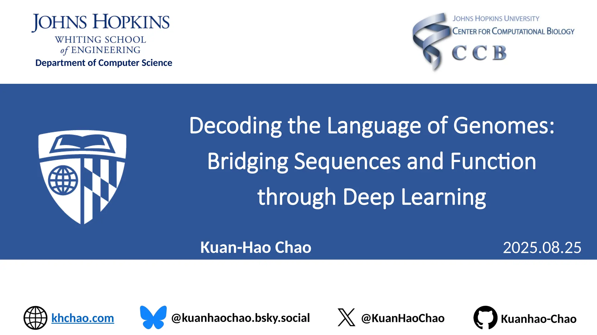
8
Assembly & Indexing
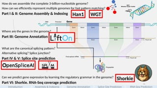
Howdo we assemble the complete 3-billion-nucleotide genome?
How can we efficiently represent multiple genomes for fast pattern matching?
Part I & II: Genome Assembly & Indexing
Where are the genes in the genome?
Part III: Genome Annotation
Can we predict gene expression by learning the regulatory grammar in the genome?
Part VI: Shorkie. RNA-Seq coverage prediction
What are the canonical splicing pattern?
Alternative splicing? Splice junction?
Part IV & V: Splice site prediction
Introduction Genome Annotation Splice Site Prediction RNA-Seq Prediction
9.
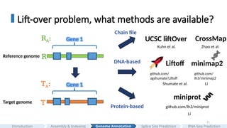
9
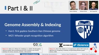
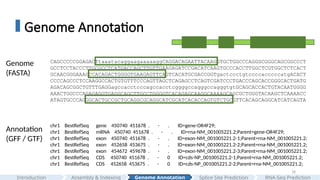
Part I &II
Genome Assembly & Indexing
• Han1: first gapless Southern Han Chinese genome
• WGT: Wheeler graph recognition algorithm
Chao, K. H., Zimin, A. V., Pertea, M., & Salzberg, S. L. (2023). The first gapless,
reference-quality, fully annotated genome from a Southern Han Chinese
individual. G3: Genes, Genomes, Genetics, 13(3), jkac321.
Chao, K. H., Chen, P. W., Seshia, S. A., & Langmead, B. (2023). WGT: Tools and
algorithms for recognizing, visualizing, and generating Wheeler graphs.
Iscience, 26(8).
Steven Salzberg Mihaela Pertea Ben Langmead
Assembly & Indexing
Introduction Genome Annotation Splice Site Prediction RNA-Seq Prediction
10.
10
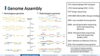
Genome Assembly
Assembly &Indexing
Introduction Genome Annotation Splice Site Prediction RNA-Seq Prediction
Li, H., Durbin, R. Genome assembly
in the telomere-to-telomere era. Nat
Rev Genet 25, 658–670 (2024).
1976 Bacteriophage MS2 ~3.5 kb
1977 Sanger sequencing
1990-2000: BAC-by-BAC shot gun strategy
2003 near-complete human genome
2000s second-generation sequencing
short-read sequencing
(Illumina)
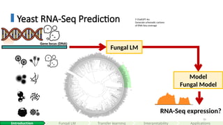
2010s third-generation sequencing
long-read sequencing
(PacBio; ONT)
2019 Telomere-to-Telomere (T2T) era
2022 First complete human genome
1972 Bacteriophage MS2 coat gene
Homozygous genome Heterozygous genome
11.
11
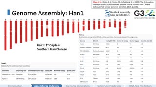
Genome Assembly: Han1
Chao,K. H., Zimin, A. V., Pertea, M., & Salzberg, S. L. (2023). The first gapless,
reference-quality, fully annotated genome from a Southern Han Chinese
individual. G3: Genes, Genomes, Genetics, 13(3), jkac321.
Han1: 1st
Gapless
Southern Han Chinese
GenBank assembly:
GCA_024586135.1
Assembly & Indexing
Introduction Genome Annotation Splice Site Prediction RNA-Seq Prediction
12.
12
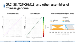
GRCh38, T2T-CHM13, andother assemblies of
Chinese genome
Mummer dot plot Gene order plot Inversion on β defensin gene cluster
Assembly & Indexing
Introduction Genome Annotation Splice Site Prediction RNA-Seq Prediction
13.
13
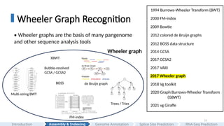
Wheeler Graph Recognition
Assembly& Indexing
Introduction Genome Annotation Splice Site Prediction RNA-Seq Prediction
2000 FM-index
2009 Bowtie
1994 Burrows-Wheeler Transform (BWT)
2012 BOSS data structure
2014 GCSA
2012 colored de Bruijn graphs
2017 VARI
2017 Wheeler graph
2017 GCSA2
2020 Graph Burrows-Wheeler Transform
(GBWT)
2021 vg Giraffe
2018 Vg toolkit
• Wheeler graphs are the basis of many pangenome
and other sequence analysis tools
Multi-string BWT
FM-index
XBWT
Trees / Tries
de Bruijn graph
Bubble-resolved
GCSA / GCSA2
BOSS
Wheeler graph
14.
14
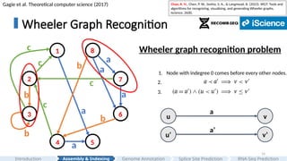
Wheeler Graph Recognition
Chao,K. H., Chen, P. W., Seshia, S. A., & Langmead, B. (2023). WGT: Tools and
algorithms for recognizing, visualizing, and generating Wheeler graphs.
Iscience, 26(8).
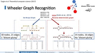
Gagie et al. Theoretical computer science (2017)
Assembly & Indexing
Introduction Genome Annotation Splice Site Prediction RNA-Seq Prediction
z
a
a
a
a
a
b
b
b
b
c
c
c
c
8
1
2
3
4 5
6
7
u v
a
u’ v’
a’
3.
2.
1. Node with indegree 0 comes before every other nodes.
Wheeler graph recognition problem
15.
15
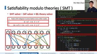
Satisfiability modulo theories( SMT )
• SMT solver = SAT solver + IDL theory solver
1 2 3 4 5 6 7 8
1 2 3 4 5 6 7 8
3.
2.
1. Node with indegree 0 comes before every other nodes.
Assembly & Indexing
Introduction Genome Annotation Splice Site Prediction RNA-Seq Prediction
Pei-Wei Chen
17
Part III
Genome Annotation
•LiftOn: genome annotation lift-over
• Application: CHESS (GRCh38 - > CHM13; GRCh38 - > Han1)
Chao, K. H., Heinz, J. M., Hoh, C., Mao, A., Shumate, A., Pertea, M., &
Salzberg, S. L. (2025). Combining DNA and protein alignments to improve
genome annotation with LiftOn. Genome Research, 35(2), 311-325.
Steven Salzberg Mihaela Pertea
Assembly & Indexing
Introduction Genome Annotation Splice Site Prediction RNA-Seq Prediction
24
Result 2: improveCHM13 protein annotations
Assembly & Indexing
Introduction Genome Annotation Splice Site Prediction RNA-Seq Prediction
25.
25
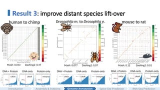
Result 3: improvedistant species lift-over
human to chimp Drosophila m. to Drosophila e. mouse to rat
Liftoff miniprot
LiftOn Liftoff miniprot
LiftOn
Liftoff miniprot
LiftOn
DNA + Protein DNA-only Protein-only DNA + Protein DNA-only Protein-only
DNA + Protein DNA-only Protein-only
Mash: 0.013 Dashing2: 0.47 Mash: 0.12 Dashing2: 0.01
Mash: 0.077 Dashing2: 0.07
Assembly & Indexing
Introduction Genome Annotation Splice Site Prediction RNA-Seq Prediction
27
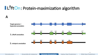
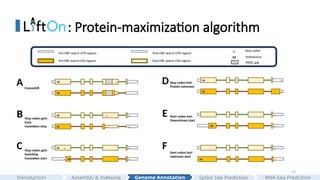
: Protein-maximization algorithm
Liftoffprotein alignment
miniprot protein alignment
- - - - - - -
- - - --
Reference protein
Liftoff protein
miniprot protein INDEL
mismatch Stop codon
*
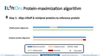
Step 1: Align Liftoff & miniprot proteins to reference protein
B
*
Assembly & Indexing
Introduction Genome Annotation Splice Site Prediction RNA-Seq Prediction
28.
28
: Protein-maximization algorithm
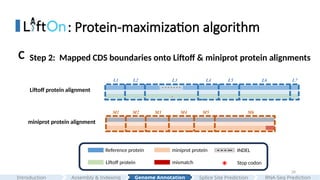
Step2: Mapped CDS boundaries onto Liftoff & miniprot protein alignments
C
Liftoff protein alignment
miniprot protein alignment
- - - - - - -
*
- - - --
Reference protein
Liftoff protein
miniprot protein INDEL
mismatch Stop codon
*
M1 M2 M3 M5 M6
M4
L1 L2 L3 L5 L6 L7
L4
Assembly & Indexing
Introduction Genome Annotation Splice Site Prediction RNA-Seq Prediction
29.
29
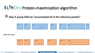
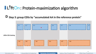
: Protein-maximization algorithm
LiftOnCDS chaining
L3 L5 L6 L7
M1 M2 M3 M5 M6
L2
M4
L1 L4
*
Step 3: group CDSs by “accumulated AA in the reference protein”
D
Assembly & Indexing
Introduction Genome Annotation Splice Site Prediction RNA-Seq Prediction
30.
30
: Protein-maximization algorithm
LiftOnCDS chaining
L3 L5 L6 L7
M1 M2 M3 M5 M6
L2
M4
L1 L4
*
Step 3: group CDSs by “accumulated AA in the reference protein”
D
Assembly & Indexing
Introduction Genome Annotation Splice Site Prediction RNA-Seq Prediction
31.
31
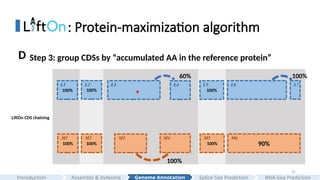
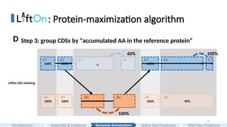
: Protein-maximization algorithm
LiftOnCDS chaining
100%
100% 100% 100% 90%
L3 L5 L6 L7
M1 M2 M3 M5 M6
100%
L2
M4
100%
L1 L4
*
Step 3: group CDSs by “accumulated AA in the reference protein”
D
100%
60% 100%
Assembly & Indexing
Introduction Genome Annotation Splice Site Prediction RNA-Seq Prediction
32.
32
: Protein-maximization algorithm
LiftOnCDS chaining
100%
100% 100% 100% 90%
L3 L5 L6 L7
M1 M2 M3 M5 M6
100%
L2
M4
100%
L1 L4
100%
60%
*
100%
Step 3: group CDSs by “accumulated AA in the reference protein”
D
Assembly & Indexing
Introduction Genome Annotation Splice Site Prediction RNA-Seq Prediction
33.
33
: Protein-maximization algorithm
Stopcodon gain:
Early
translation stop
M
M
*
*
*
*
B
M
M
*
*
Stop codon lost:
Protein extension
D
Start codon lost:
Downstream start
M
*
*
E
M
*
*
Start codon lost:
Upstream start
F
A Frameshift
M
*
--
--
*
M
Pre-ORF search UTR regions
Pre-ORF search CDS regions
*
M
Post-ORF search UTR regions
Post-ORF search CDS regions
Stop codon
Methionine
-- INDEL gap
C Stop codon gain:
Switching
translation start
*
*
M
M
*
*
Assembly & Indexing
Introduction Genome Annotation Splice Site Prediction RNA-Seq Prediction
34.
34
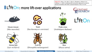
: more lift-overapplications
House mouse
(Mus musculus)
Rice
(Oryza sativa)
Thale cress
(Arabidopsis thaliana)
Honey bee
(Apis mellifera)
fruit fly
(Drosophila melanogaster)
Yeast
(Saccharomyces cerevisiae)
Assembly & Indexing
Introduction Genome Annotation Splice Site Prediction RNA-Seq Prediction
Chao, K. H., Heinz, J. M., Hoh, C., Mao, A., Shumate, A., Pertea, M., &
Salzberg, S. L. (2025). Combining DNA and protein alignments to improve
genome annotation with LiftOn. Genome Research, 35(2), 311-325.
35.
35
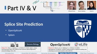
Part IV &V
Splice Site Prediction
• OpenSpliceAI
• Splam
Chao, K. H., Mao, A., Salzberg, S. L., & Pertea, M. (2024). Splam: a deep-
learning-based splice site predictor that improves spliced alignments.
Genome biology, 25(1), 243.
Chao, K. H., Mao, A., Liu, A., Salzberg, S. L., & Pertea, M. (2025).
OpenSpliceAI: An efficient, modular implementation of SpliceAI enabling easy
retraining on non-human species. eLife, 2025-03.
Mihaela Pertea Steven Salzberg Anqi Liu
Assembly & Indexing
Introduction Genome Annotation Splice Site Prediction RNA-Seq Prediction
36.
36
Splice Site Prediction
Genelocus (DNA)
Transcription
Model
Where are the splice sites?
🤖 ChatGPT 4o:
Generate
schematic cartoon
of RNA splicing
Assembly & Indexing
Introduction Genome Annotation Splice Site Prediction RNA-Seq Prediction
37.
37
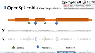
: Splice siteprediction
AGACTCAGCCCCCGGAGACTTAGTTAGAGGAAGAAAAAGGTAGGACAGAAGAAAAAGGCAGGACATACAAGGTGCTGGCCCAGGGCGG
X
Y 000000000000000000000200000001000000002000000000000100000000000000000000000000000000000
Donor: 2 Acceptor: 1 Neither: 0
Assembly & Indexing
Introduction Genome Annotation Splice Site Prediction RNA-Seq Prediction
Chao, K. H., Mao, A., Liu, A., Salzberg, S. L., & Pertea, M.
(2025). OpenSpliceAI: An efficient, modular implementation of
SpliceAI enabling easy retraining on non-human species. eLife
38.
38
𝑊 =5000𝐹=10,000
𝐿=33200
𝐿=14600
𝐿=25000
Gene 1
Gene2
Gene n
…
Raw gene DNA sequence
[7, 15000, 4]
[3, 15000, 4]
[5, 15000, 4]
[7, 5000, 3]
[3, 5000, 3]
[5, 5000, 3]
X Y
…
~20k protein-coding genes
Assembly & Indexing
Introduction Genome Annotation Splice Site Prediction RNA-Seq Prediction
39.
39
: retrain ondifferent species
System time Memory GPU Avg memory
Assembly & Indexing
Introduction Genome Annotation Splice Site Prediction RNA-Seq Prediction
40.
40
: ISM &variant prediction
SpliceAI
OpenSpliceAI
OPA1 (chr3:193644727A>G) OpenSpliceAI Score
Acceptor Site Score Donor Site Score
A G T G A G G T A G A A A
C
0.099
5’
5’
3’
3’
Reference
Mutated
A A G G G T A A
G 54 bp
A G T G A G G T A G G A A C
A A G G G T A A G
0.989
0.343
0.985
(Qian et al., 2021)
SpliceAI Score
0.093
0.970
0.247
0.982
Assembly & Indexing
Introduction Genome Annotation Splice Site Prediction RNA-Seq Prediction
Alan Mao
41.
41
: predicting splicesites in a pair
Exon Exon Exon Exon Exon
Intron Intron Intron Intron
Donor Acceptor
Splice junction
Donor: 400bp Acceptor: 400bp
Assembly & Indexing
Introduction Genome Annotation Splice Site Prediction RNA-Seq Prediction
Chao, K. H., Mao, A., Salzberg, S. L., & Pertea, M. (2024).
Splam: a deep-learning-based splice site predictor that
improves spliced alignments. Genome biology, 25(1), 243.
Data
43
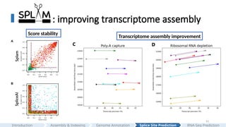
: improving transcriptomeassembly
C D
Score stability
Transcriptome assembly improvement
Assembly & Indexing
Introduction Genome Annotation Splice Site Prediction RNA-Seq Prediction
44.
44
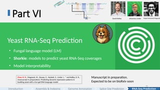
Part VI
Yeast RNA-SeqPrediction
• Fungal language model (LM)
• Shorkie: models to predict yeast RNA-Seq coverages
• Model interpretability
Chao, K. H., Magzoub, M., Stoops, E., Hackett, S., Linder J., * and Kelley, D. R.,
(manuscript in preparation). Predicting dynamic expression patterns in
budding yeast with a fun-gal DNA language model
Manuscript in preparation.
Expected to be on bioRxiv soon
David Kelley Johannes Linder Majed Mohamed Magzoub
Assembly & Indexing
Introduction Genome Annotation Splice Site Prediction RNA-Seq Prediction
45.
45
Questions we answerin this study:
Main Goal
• Predict yeast gene expression (RNA-Seq coverage)
directly from DNA sequences.
Interpretability
Introduction Fungal LM Transfer learning Applications
Assembly & Indexing
Introduction Genome Annotation Splice Site Prediction RNA-Seq Prediction
46.
46
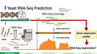
Yeast RNA-Seq Prediction
Readsalignment
Coverage pileup
Reads
mRNA
Gene expression
model
RNA-Seq expression?
Gene locus (DNA)
🤖 ChatGPT 4o:
Generate schematic
cartoon of RNA-Seq
🤖 ChatGPT 4o:
Generate schematic cartoon
of RNA-Seq coverage
Interpretability
Introduction Fungal LM Applications
Transfer learning
47.
47
Yeast RNA-Seq Prediction
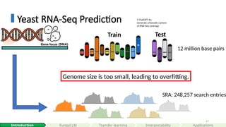
Genelocus (DNA)
🤖 ChatGPT 4o:
Generate schematic cartoon
of RNA-Seq coverage
Interpretability
Introduction Fungal LM Applications
Train Test
12 million base pairs
SRA: 248,257 search entries
Genome size is too small, leading to overfitting.
Transfer learning
48.
48
Yeast RNA-Seq Prediction
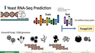
Genelocus (DNA)
🤖 ChatGPT 4o:
Generate schematic cartoon
of RNA-Seq coverage
Interpretability
Introduction Fungal LM Applications
Train Test
12 million base pairs
Ensembl fungi: 1500 genomes
Fungal LM
Transfer learning
49.
49
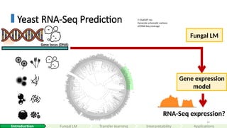
Yeast RNA-Seq Prediction
Geneexpression
model
Gene locus (DNA)
🤖 ChatGPT 4o:
Generate schematic cartoon
of RNA-Seq coverage
Interpretability
Introduction Fungal LM Applications
Fungal LM
RNA-Seq expression?
Transfer learning
50.
50
Yeast RNA-Seq Prediction
Model
FungalModel
Gene locus (DNA)
🤖 ChatGPT 4o:
Generate schematic cartoon
of RNA-Seq coverage
Interpretability
Introduction Fungal LM Applications
Fungal LM
RNA-Seq expression?
Transfer learning
52
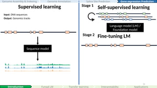
Sequence model
Supervised learning
Input:DNA sequences
Output: Genomics tracks
Interpretability
Introduction Fungal LM Applications
Genome Assembly & Indexing Genome Annotation Gene expression Prediction
Splice Site Prediction
Transfer learning
53.
53
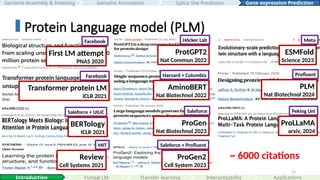
First LM attempt
PNAS2020
Facebook
Transformer protein LM
ICLR 2021
Facebook
BERTology
ICLR 2021
Saleforce + UIUC
Review
Cell Systems 2021
MIT
ProtGPT2
Nat Commun 2022
Höcker Lab
AminoBERT
Nat Biotechnol 2022
Harvard + Columbia
ProGen
Nat Biotechnol 2023
Saleforce
ProGen2
Cell System 2023
Saleforce + Profluent
ESMFold
Science 2023
Meta
PLM
Nat Biotechnol 2024
Profluent
ProLLaMA
arxiv, 2024
Peking Uni
~ 6000 citations
Interpretability
Introduction Fungal LM Applications
Protein Language model (PLM)
Genome Assembly & Indexing Genome Annotation Gene expression Prediction
Splice Site Prediction
Transfer learning
54.
54
DNABERT
Bioinformatics 2021
SBU
GPN
PNAS 2023
UCBerkeley
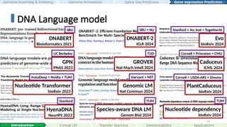
Nucleotide Transformer
bioRxiv 2023
InstaDeep + Nvidia + TUM
HyenaDNA
NeurIPS 2023
Stanford
DNABERT-2
ICLR 2024
SBU + NU
GROVER
Nat Mach Intell 2024
TUD
Genomic LM
Nat Commun 2024
Harvard + MIT
Species-aware DNA LM
Genom Biol 2024
TUM
Evo
bioRxiv 2024
Stanford + Arc Inst + TogetherAI
Caduceus
ICML 2024
Cornell + Princeton + CMU
PlantCaduceus
bioRxiv 2024
Cornell + USDA-ARS + Simons
Nucleotide dependency
bioRxiv 2024
TUM
Interpretability
Introduction Fungal LM Applications
DNA Language model
Genome Assembly & Indexing Genome Annotation Gene expression Prediction
Splice Site Prediction
Transfer learning
55.
55
Sequence model
Supervised learningSelf-supervised learning
Stage 1
Language model (LM) /
Foundation model
Input: DNA sequences
Output: Genomics tracks
Interpretability
Introduction Fungal LM Applications
Genome Assembly & Indexing Genome Annotation Gene expression Prediction
Splice Site Prediction
Stage 2 Fine-tuning LM
Transfer learning
56.
56
Language model (LM)/
Foundation model
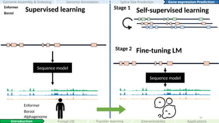
Enformer
Borzoi
Supervised learning
Stage 2
Sequence model
Fine-tuning LM
Interpretability
Introduction Fungal LM Applications
Genome Assembly & Indexing Genome Annotation Gene expression Prediction
Splice Site Prediction
Self-supervised learning
Stage 1
Sequence model
Enformer
Borzoi
Alphagenome
Transfer learning
57.
57
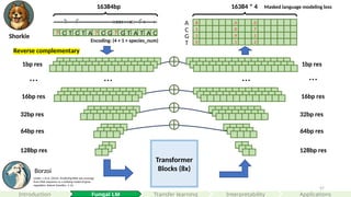
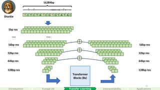
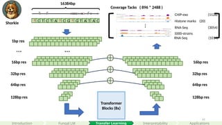
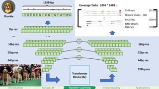
Transformer
Blocks (8x)
32bp res
64bpres
128bp res
? C T C T A ? C G ? G T A T A C
…
32bp res
64bp res
128bp res
1bp res
…
… …
16384bp
8 0 0
16384 * 4
A
C
G
T
1 0 7
1 9 1
0 1 2
.
.
.
.
.
.
.
.
.
.
.
.
16bp res 16bp res
1bp res
Reverse complementary
Masked language modeling loss
Encoding: (4 + 1 + species_num)
Linder, J. et al. (2025). Predicting RNA-seq coverage
from DNA sequence as a unifying model of gene
regulation. Nature Genetics, 1-13.
Borzoi
Interpretability
Introduction Fungal LM Applications
Transfer learning
Shorkie
58.
58
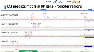
LM predicts motifsin RP gene Promoter regions
chrIV:307974-308474
chrV:396,319-396,819
RAP1.1
RAP1.1
Fhl1
chrVII:254,191-254,691 Fhl1
RAP1.1
Start codon
450 nt 50 nt
Interpretability
Introduction Fungal LM Applications
chrIV:229,456-229,956 RAP1.1 FHL1
RAP1 FHL1
Transfer learning
59.
59
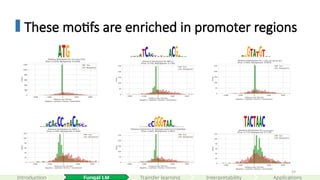
These motifs areenriched in promoter regions
start codon (ATG)
5’ splice site (donor site)
branch point
Interpretability
Introduction Fungal LM Applications
Transfer learning
60.
60
Transformer
Blocks (8x)
32bp res
64bpres
128bp res
? C T C T A ? C G ? G T A T A C
1bp res
…
32bp res
64bp res
128bp res
1bp res
…
… …
16384bp
8 0 0
16384 * 4
A
C
G
T
1 0 7
1 9 1
0 1 2
.
.
.
.
.
.
.
.
.
.
.
.
16bp res 16bp res
Shorkie
Interpretability
Introduction Transfer Learning Applications
Fungal LM
61.
61
Transformer
Blocks (8x)
32bp res
64bpres
128bp res
? C T C T A ? C G ? G T A T A C
1bp res
…
32bp res
64bp res
128bp res
…
16384bp
16bp res 16bp res
Shorkie
Interpretability
Introduction Applications
Fungal LM Transfer Learning
62.
62
Transformer
Blocks (8x)
32bp res
64bpres
128bp res
? C T C T A ? C G ? G T A T A C
1bp res
…
32bp res
64bp res
128bp res
…
16384bp
16bp res 16bp res
Shorkie
Interpretability
Introduction Applications
Fungal LM
Coverage Tacks ( 896 * 2488 )
CHiP-exo (1128)
Histone marks (20)
RNA-Seq (3054)
…
1000-strains
RNA-Seq (1014)
Transfer Learning
63.
63
Transformer
Blocks (8x)
32bp res
64bpres
128bp res
? C T C T A ? C G ? G T A T A C
1bp res
…
32bp res
64bp res
128bp res
…
16384bp
16bp res 16bp res
Shorkie
Interpretability
Introduction Applications
Fungal LM
Coverage Tacks ( 896 * 2488 )
CHiP-exo (1128)
Histone marks (20)
RNA-Seq (3054)
…
1000-strains
RNA-Seq (1014)
Transfer Learning
65
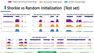
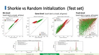
Shorkie vs RandomInitialization (Test set)
Bin level
(each dot is a track; all bins)
Gene level (each dot is a track; all genes) Track level
(each dot is a gene; all tracks)
Interpretability
Introduction Applications
Fungal LM
Gene Gene
Transfer Learning
66.
66
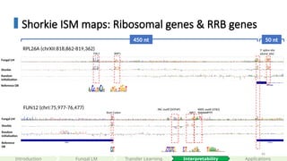
Shorkie ISM maps:Ribosomal genes & RRB genes
450 nt 50 nt
RPL26A (chrXII:818,862-819,362)
RAP1
FHL1
Fungal LM
Shorkie
Random
initialization
5’ splice site
(donor site)
Reference DB
Fungal LM
Shorkie
Random
initialization
FUN12 (chrI:75,977-76,477)
Start Codon
PAC motif (DOT6P)
ABF1
RRPE motif (STB3)
TGAAAAATTTT
Reference
DB
Interpretability
Introduction Applications
Fungal LM Transfer Learning
67.
67
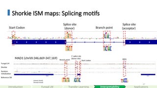
Shorkie ISM maps:Splicing motifs
MAD1 (chrVII:346,669-347,169) REB1
Start codon
5’ splice site
(donor site)
Branch point
(reverse strand)
(forward strand)
Start Codon
Splice site
(donor) Branch point
Splice site
(acceptor)
Fungal LM
Shorkie
Random
initialization
Reference DB
Interpretability
Introduction Applications
Fungal LM Transfer Learning
68.
68
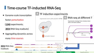
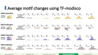
Time-course TF-inducted RNA-Seq
Interpretability
IntroductionApplications
Fungal LM Transfer Learning
● Genome-scale transcription
factor perturbation
(1340 experiments;
3054 RNA-Seq readouts)
● Aggregating dynamics across
many time-courses
3054 RNA-Seq
readouts
TF induction experiments
RNA-seq at different T
71
Introduction Applications
Fungal LMInterpretability
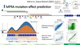
Rafi et al., Nature Biotech (2024)
RNA-Seq Coverage
Prediction
Rafi et al. Yeast
Sequences
(single-sequence)
Shorkie DREAM-RNN
MPRA mutation effect prediction
Insertion
Transfer Learning
72.
72
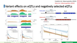
Variant effects oneQTLs and negatively selected eQTLs
Introduction Applications
Fungal LM Interpretability
Caudal et al., Nature genetics (2024)
Transfer Learning
Kita et al., Nature genetics (2024)
73.
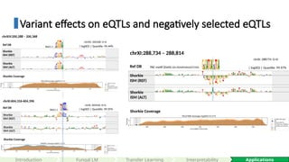
Variant effects oneQTLs and negatively selected eQTLs
Shorkie
ISM (ALT)
Shorkie
ISM (REF)
Ref DB
Shorkie Coverage
Reb1.1
chrXI: 604356: A>G
| logSED | Quantile: 99.95%
chrXI:604,316-604,396
Introduction Applications
Fungal LM Interpretability
Reb1.1
chrXIV: 200328: G>A
| logSED | Quantile: 99.44%
chrXIV:200,288 – 200,368
Shorkie
ISM (ALT)
Shorkie
ISM (REF)
Ref DB
Shorkie Coverage
chrXI: 288774: G>A
| logSED | Quantile: 99.97%
PAC motif (Dot6) G(C/A)GATGAG(A/C)TGA
chrXI:288,734 – 288,814
Shorkie
ISM (ALT)
Shorkie
ISM (REF)
Ref DB
Shorkie Coverage
Transfer Learning
74.
74
Assembly & Indexing
Howdo we assemble the complete 3-billion-nucleotide genome?
How can we efficiently represent multiple genomes for fast pattern matching?
Part I & II: Genome Assembly & Indexing
Where are the genes in the genome?
Part III: Genome Annotation
Can we predict gene expression by learning the regulatory grammar in the genome?
Part VI: Shorkie. RNA-Seq coverage prediction
What are the canonical splicing pattern?
Alternative splicing? Splice junction?
Part IV & V: Splice site prediction
Introduction Genome Annotation Splice Site Prediction RNA-Seq Prediction
Han1 WGT
Shorkie
75.
75
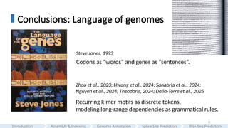
Conclusions: Language ofgenomes
Codons as “words” and genes as “sentences”.
Recurring k-mer motifs as discrete tokens,
modeling long-range dependencies as grammatical rules.
Steve Jones, 1993
Zhou et al., 2023; Hwang et al., 2024; Sanabria et al., 2024;
Nguyen et al., 2024; Theodoris, 2024; Dalla-Torre et al., 2025
Assembly & Indexing
Introduction Genome Annotation Splice Site Prediction RNA-Seq Prediction
76.
76
Conclusions: Language ofgenomes
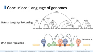
Natural Language Processing
DNA gene regulation
Kornblihtt et al.
Assembly & Indexing
Introduction Genome Annotation Splice Site Prediction RNA-Seq Prediction
77.
77
Conclusions: Language ofgenomes
Assembly & Indexing
Introduction Genome Annotation Splice Site Prediction RNA-Seq Prediction
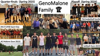
85
AC Malone (Sum2023)
TSA basketball family
Softball (Sum 2023)
GenoMalone
Family 🏆
🏆
JHU X UMD Sport Day
Quarter-finals (Spring 2025) Playoff (Spring 2024)
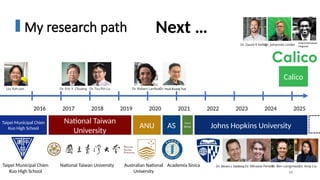
My research path
88
TaipeiMunicipal Chien
Kuo High School
National Taiwan University Academia Sinica
2016 2017 2018 2019 2020 2021 2022 2023 2024 2025
National Taiwan
University
ANU AS Johns Hopkins University
Calico
Taipei Municipal Chien
Kuo High School
Australian National
University
Next …
Taiwan
Army
Liu Yuh-san Dr. Eric Y. Chuang Dr. Tzu-Pin Lu Dr. Huai-Kuang Tsai
Dr. Robert Lanfear
Dr. Steven L Salzberg Dr. Mihaela Pertea
Dr. Ben Langmead
Dr. Anqi Liu
Dr. David R Kelley
Dr. Johannes Linder
Majed Mohamed
Magzoub
89.
89
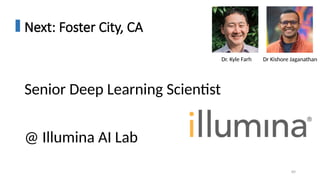
Next: Foster City,CA
Senior Deep Learning Scientist
@ Illumina AI Lab
Dr. Kyle Farh Dr Kishore Jaganathan
Editor's Notes
#1 Thank you Steven, thank you Ela for you kind introduction.
And thank you for your mentorship throughout the past four years.
Good afternoon everyone.
Thank you all for being here and on Zoom
I’m grateful to my committee, friends, and family.
Your guidance and support made this work possible.
My dissertation is titled “Decoding the Language of Genomes: Bridging Sequences and Function through Deep Learning.”
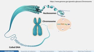
#2 The story starts with a cell. Cell is the fundamental unit of life.
Our bodies are made of tens of trillions of cells. They come in all shapes and sizes—
[CLICK]
from thin, sheet-like endothelial cells to gigantic, multi-nucleated muscle fibers.
Yet despite these differences, every cell carries the same genetic blueprint: DNA,
[CLICK]
stored inside the nucleus, separated from the cytoplasm.
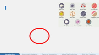
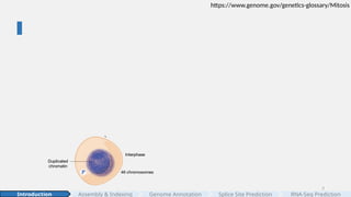
#3 To pass along genetic information, cells duplicate and divide, and this process is called mitosis. [click]
#4 Mitosis preserves the instructions for life from one generation of cells to the next.
And to move meters of DNA without tangling, the cell compacts DNA hierarchically.
#5 At its most compact level, chromosomes are highly condensed that we can see them under a light microscope.
Between divisions, chromosomes relax into chromatin: long stretches of DNA organized into higher-order fibers (often called chromatin fibers).
[click]
Zooming in, those fibers resolve into arrays of nucleosomes—the classic “beads on a string.”
[click]
Each nucleosome contains ~147 base pairs of DNA wrapped 1.7 turns around a histone octamer, joined by short stretches of linker DNA.
[click]
#6 Zooming in further, at the molecular level, DNA is a double helix of two antiparallel strands held together by A–T and G–C base pairs. [click]
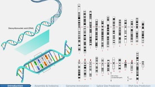
In humans, these sequences are organized into 23 chromosome pairs—one set from each parent—carrying the full blueprint of our genome. [click]
“How much information is that?”
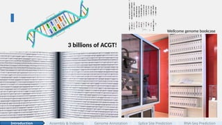
#7 In total the human genome spans about 3 billion nucleotides—A, C, G, and T.
Here’s a visualization of its sheer size:
<CLICK> if we were to print out the entire human genome in books, each page would look something like this, and the complete set would span 109 books, each containing hundreds of pages. Very impressive!
And these 3 billion nucleotides set the stage for the questions my dissertation addresses.”
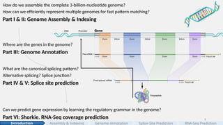
#8 Within this vast, information-dense sequence of 3 billion nucleotides, we can ask many questions at different levels.
[click]
First, CAN we build the genome and can we represent many genomes for fast search? That’s Parts 1 & 2—assembly and indexing.
[click]
Next, where are the genes and what are their structures in the genome? That’s Part 3—genome annotation.
[click]
and moving on to the function, as transcripts are processed, introns are removed and exons joined. Mature RNAs are being generated. What are the canonical and alternative splicing patterns, and can we build model to predict cryptic splicing? That’s Parts 4 & 5—splice-site prediction.
[click]
Finally, if we combine these layers of gene regulation, can we learn the ‘regulatory grammar’ in DNA well enough to predict expression? That’s Part 6—RNA-Seq coverage prediction.
#9 The genome is the foundation of all downstream genomic analyses.
And the process of stitching short-read and long-read sequences into contigs and scaffolds,
turning raw sequencing data into a coherent reference, is called genome assembly.
#10 Here is a brief history of genome assembly over five decades.
It began in 1972 with the first attempt to assemble the MS2 coat protein-coding gene, followed by the breakthrough of Sanger sequencing.
In the 1990s, the Human Genome Project used a BAC-by-BAC shotgun sequencing approach to sequence the human genome, producing the first near-complete draft in 2003.
In early 2000s, Short-read sequencing technologies drove sequencing costs down substantially; and later on long-read sequencing approaches made telomere-to-telomere assembly possible.
Finally in 2022, scientists have finally assembled the first complete human genome, T2T-CHM13 led by the T2T consurtium. marking the milestone in human history.
[CLICK]
With more accurate and longer sequencing methods available, now we are entering the era of assembling more gapless, reference-quality homozygous genomes, or even heterozygous diploid genomes from diverse individuals.
#11 And In genome assembly field, I assembled and annotated the first gapless southern chinese Han genome, and we called it han1.
Here is a ideograms of all the chromosomes, wit the red regions directly assembled from HG0621, and the pink region were inserted from T2T-CHJM13.
#12 And then we compared the assembled Han1 genome to T2T-CHM13.
In the mummer dot plot and gene order plot, we can see two genomes are highly colinear to each other.
One interesting finding is that Han1 contains a large 4 mega base pairs of inversion on beta defensin gene cluster at chr8 compared to T2T-CHM13.
Genome assembly allows us to see these large indels.
In part 1, we demonstrate that entering the T2T era, by leveraging ultra-long Oxford Nanopore and PacBio reads, with the guide of T2T-CHM13, any lab with sufficient long-read coverage can generate gapless, reference-quality human genomes from diverse ancestries.
#13 We’ve built the reference—now the practical question is: how do we search it fast?
Indexing answers this by organizing one or many genomes into compact, searchable data structures, so alignment, pattern matching, and sequence comparison become tractable at scale.
On linear references, the story begins with the Burrows–Wheeler Transform and the FM-index, which together enable fast, memory-efficient pattern matching.
[click]
As we move from one genome to many, graph indexes emerge: for example, colored de Bruijn graphs to track k-mer presence across samples; and their succinct data strucutre -- BOSS; and path indexes like GCSA/GCSA2 for searching walks in a graph.
[click]
And if you look into their “state diagram,” you'll find that they share some similarities. In 2017, Gagie et al proposed a unifying framework call Wheeler graph.
#14 A Wheeler graph is an edge-labeled directed graph whose vertices admit a total ordering such that, for any pair of edges, the following three rules hold.
[CLICK]
First, nodes with indegree 0 comes before every other nodes.
Next: compare two edges by label.
• If one edge has a smaller label (a < a′), its destination must come earlier than the other’s (v < v′).
• Finally: if the edge labels tie (a = a′), preserve source order: if the source u comes before u′, then the destination v must not bigger than v’.
And the Wheeler graph recognition problem is NP complete.
#15 And in this work, we propose a new recognition algorithm that combines renaming heuristics with an SMT solver to elegantly and efficiently recognize a given graph is Wheeler or not in the order of thousands of nodes and edges.
[CLICK]
Here is a quick walk through of the implementation.
#16 Here is one example of the advantage of Wheeler-graph index.
Given a multiple sequence alignment, we can either build a popular de Bruijn graph or start with a GCSA2 graph and then massage the graph, unzip bubbles to obtain a Wheeler graph that gives us desirable property of fast pattern matching. And this representation potentially can be spatially more efficient.
In Part 2, we introduce WGT, the first open-source toolkit for generating, recognizing, and visualizing Wheeler graphs. At its core is a new algorithm that combines a permutation-based heuristic with an SMT solver to efficiently determine Wheeler orderings. This work establishes a foundational recognition algorithm concept for next-generation pangenome indexing.
#17 After we have a high-quality genome assembly, the next step is to annotate the functions of the genome.
Genome annotation is the process of identifying and marking the locations and functions of genes, as well as other important features such as promoters, enhancers, and 5' 3' untranslated regions and so on, within a genome.
#18 Here is an example. It is an annotation of a gene locus on chromosome 1, with a single protein-coding transcript, composed of three exons and two CDSs.
The annotation provides the accurate exon-intron boundaries within a gene
Genome annotation involves a combination of computational predictions, experimental verification, and manual refinement.
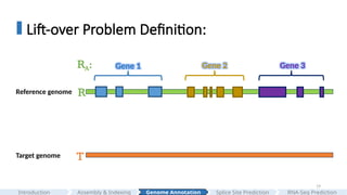
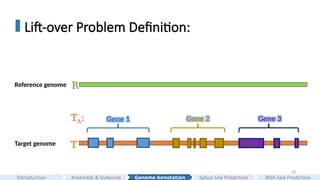
#19 Imagine you have assembled a new genome and would like to annotate it.
Instead of repeating these complicated processes and annotating them from scratch, a more efficient approach is to transfer genes from a previously well-annotated, high-quality genome to your assembly. This problem is known as annotation lift-over.
A more formal definition is as follows:
Given a reference genome R, and the reference annotation R_A,
Our goal is to change the coordinates of the genes from the reference genome to the target genome, and generate the target annotation TA.
#20 Our goal is to change the coordinates of the gene loci from the reference genome to the target genome, and generate the target annotation TA.
#21 What are some methods that are available for converting genomic feature coordinates?
One approach is to pre-generate a chain file for example like UCSC liftOver and CrossMap.
However, this approach often splits mappings. For instance, a gene interval might be split and mapped across different chromosomes or strands, and independent genomics feature mapping instead of doing at the gene level all together can result in exons not forming meaningful transcripts or multiple exons in paralogous genes map to the same locus, causing inaccuracies.
Instead of using pre-generated ‘chain’ file, another approach for converting genomic feature coordinates is to lift-over genes locus by locus.
Liftoff is a DNA-based approach that uses minimap2 DNA aligner to transfer genes
And another approach is using protein aligner for example exonerate,GenSeqer, miniprot and so on.
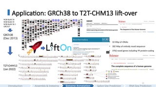
#22 In terms of application, a very great example and demonstration is T2T-CHM13 annotation. It was generated by transferring annotations from GRCh38 to CHM13.
In April 2003, scientists announced the completion of the Human Genome Project.
I quoted the word "finish" here , because, at that time, about 15% of the genome sequence was still missing. Nearly 20 years after that, the most recent reference genome still lacks about 8% of the sequence or contains errors.
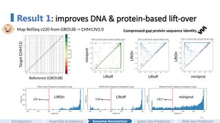
#23 So here is the first result
First, we generated LiftOn's CHM13 genome annotation by mapping genes from GRCh38 to CHM13. The protein-coding gene order plot shows that the two genomes are highly collinear with each other, as expected.
In comparing to LiftOn, we selected two state-of-the-art tools for our analysis: "Liftoff", which is a DNA-based liftover" tool, and "miniprot" for "protein-based liftover".
We then evaluated all protein-coding transcript in the genome using "compressed-gap protein sequence identity". Each dot represents a protein. It is calculated using the metrics that I just mentioned; if a dot is on the upper left panel, it means that miniprot generates a better annotation that preserves a longer protein, and vice versa.
Here you can see that no single tool is universally optimal.
Here are the results comparing LiftOn to Liftoff and miniprot, and we can see that LiftOn outperforms both.
Then, we plotted the protein sequence identity frequency plots of all proteins in the genome, and the results show that LiftOn has the least truncated protein.
In summary, LiftOn provides superior annotations, outperforming the best existing DNA-based and protein-based lift-over methods.
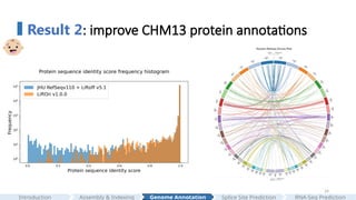
#24 We then compared the overall LiftOn's annotation to the latest released CHM13 annotation generated by Liftoff. We again observed that LiftOn produces less truncated proteins.
Furthermore, LiftOn is able to identify extra copies of genes. The circos plot here shows the relative positions of extra genes found between the target genome (on the left half of the circle) and the reference genome (on the right half of the circle).
we can see that most additional copies of genes are on the same chromosome.
#25 The third major improvement of LiftOn is its capability to map annotations between relatively distant species.
We mapped the RefSeq human annotation from human to chimpanzee, from RefSeq mouse annotation from mouse to rat, and from drosophila melanogaster to drosophila erecta
The gene order plot illustrates the genomic divergence between the two species. From left to right, the two species become more divergent and distant.
We also evaluated the genome distance by calculating the Mash distance and the Dashing2 similarity score.
#26 1. Let's walk through the workflow of our algorithm:
2. In this visualization, the blue transcript represents the correct expected annotation. Liftoff's annotation is displayed in green, while miniprot's annotation is shown in orange.
3.We can see a discrepancy between Liftoff and miniprot between the third and fourth CDSs.
4.Furthermore, we also observed that miniprot does not create a gap and misses the last splice junction and CDS, which is one of the most common mistakes that miniprot makes.
#27 In the First step , we extracted proteins from each annotation. Then, we performed pairwise alignments of the proteins from Liftoff and miniprot with the reference proteins.
Here you can see that the incorrect splice junction in Liftoff annotation introduces a premature stop codon in the Liftoff protein.
And, the miniprot alignment has a mismatch in the end of the protein sequence alignment due to the missing of the last small CDS.
#28 Then, we mapped the CDS boundaries onto the protein alignments and adjusted boundaries with CIGAR string.
#29 We group CDSs based on the numbers of the accumulated amino acids in the reference protein.
#30 Here is more details.
The grouping process begins with the first CDS in each annotation and continues until reaching the endpoints of the downstream CDS, where the number of aligned amino acids from the reference protein is the same in Liftoff and miniprot.
This forms the first CDS group in Liftoff and miniprot.
In this case, only a single CDS is included in both liftoff and minipt
Subsequent groups start from the previous endpoint in both Liftoff and miniprot, extending until the number of aligned amino acids from the reference protein matches for both annotations again.
In this case,
The grouping process concludes upon reaching the last CDS in both annotations
#31 After grouping, LiftOn calculates the partial protein sequence identity score to the reference protein for each CDS group.
We can see that the third CDS group, Liftoff has a partial score 60% due to a premature stop codon, and miniprot has a “perfect” partial protein sequence identity score.
In the fifth CDS group, since miniprot fails to generate the last small CDS, and thus has mismatches and lower protein sequence identity score.
#32 The algorithm iterates through each group and select the one with the higher score
In this example, The algorithm is able to chain the correct CDSs from Liftoff, miniprot and Liftoff
, and produce a protein annotation that achieves 100% protein sequence identity on the target genome.
LiftOn is able to select the correct regions among Liftoff and miniprot.
#33 Even though the genes are lifted over and CDSs are cahined fixed, it is possible that there are mutations in the reference genome that may interrupt the valid ORF.
LiftOn
- Searches ORFs in three frames
- Selects protein with highest sequence identity compared to reference
The frameshift or single nucleotides mutation may introduce a premature stop codons.
We adjust the CDS boundaries either to upstream stop or downstream start.
We also fix ORF for stop codon lost and start codon lost mutations.
The overall goal is to maintain the integrity of ORF for each protein-coding gene after the liftover process
#34 We expanded our experiments to various species to demonstrate LiftOn's robustness. These species include mice, yeast, honeybees, fruit flies, Arabidopsis thaliana, and rice.
In Part 3, we introduce LiftOn, a hybrid liftover tool that combines protein-to-genome alignment (via miniprot) with DNA-homology–based mapping (via Liftoff).
Our protein-maximization algorithm refines exon boundaries, corrects frameshifts, and identifies additional gene copies.
Across divergent assemblies, LiftOn yields more complete and accurate gene models than either approach alone can achieve, enabling robust cross-species annotation transfer—even for distantly related genomes.
#35 Up to now, we’ve focused on genome annotation.
[CLICK]
Genome annotation, however, depends critically on precise delineation of splice junctions—the donor, acceptor, and branch point, that together specify exon–intron gene structures.
To learn the local patterns by which Spliceosome recognizes splice sites, and to interpret variants that create cryptic splicing —we turn to splice-site prediction.
In the next section, I will describe how we predict splice sites from the DNA primary sequences and how these predictions feed back to improve transcriptome assembly and genome annotations.
#36 After a gene is transcribed, pre-mature RNA is spliced by the spliceosome.
[CLICK]
The spliceosome is a large ribonucleoprotein complex composed of five small nuclear RNAs and many proteins
[CLICK]
Step 1: the spliceosome binds to the 5’ site and branch-point, forming a phosphodiester bond and creating a loop, that is known as lariat.
[CLICK]
Step 2: the exons are ligated at the 3′ splice site, and the intron lariat is released, producing a mature mRNA, and this happens co-transcriptionally.
[CLICK]
So now the question is: can we build a model that predicts where these splice sites occur?
#37 Let's convert this biology problem into a machine learning problem.
Given a pre-mRNA sequence, a string composed of a list of ACGT alphabets. This is our X.
For each position, we can label donor sites as 2, acceptor sites as 1, and neither as 0. This is our Y.
Now the problem is transformed into a Seq to Sequence model.
#38 Now zoom out to the full genome annotation, we focus only on the protein coding genes, and we get around 19 thousand to 20 thousand protein-coding genes.
Using the same sliding-window chunking approach, we can convert them into X-y pairs.
And now we can use them to stochastically train our SpliceAI.
SpliceAI is great, however, there are some limitations.
It’s developed in Python 2.7, which make it hard to rerun and retrain.
It’s depending on old version of Keras and tensorflow.
Most important of all, it was trained on an old version of GENCODE annotation.
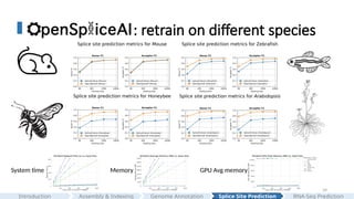
#39 Furthermore, we retrained OpenSpliceAI for four different species, mouse, zebrafish, arabidopsis thaliana, and honeybee.
For mouse, it’s relatively the closest species to human among these four species. The green curve is the model trained by OpenSpliceAI, and the blue curve is the original model. For the original spliceai model, We can see that recall remains, but precisions drop under model trained under four different flanking sequences,
For other more distant species, both precision and recall drop.
the results show that we need to retrain SpliceAI model on their specific annotation.
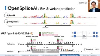
#40 So what exactly does the model learned?
In this example, the model predict => an acceptor site.
U2SURP gene.
One of our very exciting findings is a mutation in OPA1 gene.
Qian et al. reported in 2021 that an intronic splicing mutation in the OPA1 gene causes a novel cryptic exon upstream
We then did this experiment in silico, by introducing this mutation to the sequence and predicit by OpenSpliceAI.
It implies that the model learned the general splicing patterns, and it's able to predict cryptic splicing.
In part 4, I introduce OpenSpliceAI, an open-source PyTorch reimplementation of SpliceAI that preserves its state-of-the-art accuracy while offering faster inference, a reduced memory footprint, and seamless species-specific retraining. Its modular design and calibrated probability outputs simplify integration into modern workflows, like pathogenic variant screening.
Finally, ISM analyses confirm that it learns the biologically meaningful splicing motifs and predicts cryptic splicing.
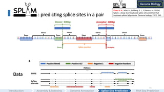
#41 Splicing isn’t that easy. One of the biggest concerns we have about SpliceAI is it's "canonical transcript labelling approach". It only selects one isoform, the canonical transcript, for labelling.
<Here is an example>
We observed that SpliceAI gives very low scores for some of the alternative splice sites.
If you are using SpliceAI to analyze your Splice junctions, you will miss a lot of alternative splice junctions.
Therefore, I developed SPLAM to learn the local regions around pairs of splice sites to determine whether a given splice junction is good or not.
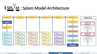
#42 This is the model architecture of Splam. It's a good example to introduce how people usually design their CNN models in modern deep learning.
This is how we design splam
#43 In part 5, I introduce Splam, a compact residual convolutional neural network designed to predict paired donor–acceptor splice sites using 400 nucleotides of flanking sequence around donors and acceptors. By operating at the splice-junction level, Splam achieves higher precision and faster inference than larger models,
and its per-junction confidence scores can be used to directly filter spliced alignments, thereby improving transcriptome assembly.
#44 Having established splice-site prediction, we now move from discrete boundary calls to quantitative modeling of transcript output: RNA-seq coverage prediction.
[skip]
Unlike splice site boundary detection, coverage prediction integrates more layers of regulation, including transcription initiation and elongation, co-/post-transcriptional processing, and mRNA stability/decay—capturing more complex gene regulation in a single quantitative readout.
#45 Predicting gene expression levels from DNA sequence is a fundamental challenge in genomics with broad implications for understanding gene regulation and disease.
Saccharomyces cerevisiae ( the budding yeast) has served as the premier model for eukaryotic gene regulation, with ~7,000 genes controlled by hundreds of transcription factors (TFs).
#46 Here is the experiment setup.
We can use a technique called "RNA Sequencing" to measure the expression of genes.
<CLICK>
First, we extracted all transcribed mRNAs in cells under a specific experiment condition, reverse-transcribed them into cDNA library.
Then we put them into a high throughput sequencing machine,
<CLICK>
This process yields millions of short reads
We then align back them back to the genome.
<CLICK>
Which gives us coverage pileups.
Essentially, RNA-Seq gives us a snapshot of which parts of the genome are actively transcribed and how genes are expressed.
<CLICK>
Our goal is to build a model to predict the RNA-Seq coverage directly from the DNA sequecnes.
#47 So, one approach is that we can simply take the reference yeast genome,
train on some chromosomes of the genome and then test on the held-out chromosomes.
[CLICK]
But here’s the challenge: the yeast genome is very compact—only about 12 megabases in total.
With such limited sequence diversity,
[CLICK]
even though we have many RNA-Seq readouts for budding yeast,;
[CLICK]
a purely supervised learning setup tends to overfit and struggles to generalize well.
#48 Fortunately, we now have access to thousands of high-quality fungal genomes. This opens the door to a different strategy: training masked DNA language models.
[CLICK]
By adopting a self-supervised pre-training approach, we can construct a fungal DNA foundation model that learns motifs, spacing preferences, and where the genes are without relying on labels.
#49 Here is the phylogenetics trees of thousands of fungal genomes that we adopted to train our fungal language model.
We found that, training with a subset of related genome with good diversity, in this case, 165 genomes in the Sachoramycetales order, we are able to achieve the best performance, preserving generalizability while avoiding overfitting.
#50 After the model gets trained
We could fine-tune the DNA language model to help with the RNA-Seq coverage predictive model.
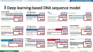
#51 Here is an overview of the extensive body of work applying standard supervised deep learning approaches to DNA sequences, particularly in the area of gene regulation
Back in 2015, DeepSEA and DeepBind were among the first works to introduce deep learning-based models for DNA sequences.
Other important tasks include using Hi-C data to predict the 3D genome organization from DNA sequences, as well as chromatin profile prediction.
Most deep learning models are CNN-based, with newer models incorporating transformer blocks.
These newer deep models aim to go beyond epigenetics to directly predict gene expression from DNA sequences.
These include the state-of-the-art models such as Enformer, Borzoi, and Alphagenome.
all four types of genome-wide tracks, including CAGE measuring transcriptional activity, histone modifications, TF binding, and DNA accessibility in various cell types and tissues for held-out chromosomes
predicts 5,313 genomic tracks for the human genome and 1,643 tracks for the mouse genome, each of length 896 corresponding to 114,688 bp aggregated into 128-bp bins.
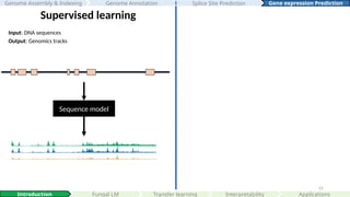
#52 This is a schematic plot of the current paradigm of supervised learning, where we paired DNA sequences to there corresponding genomics datasets predicting at different nucleotide resolutions.
#53 There has been a growing body of work applying language models to genomics, particularly in protein sequences. Notable examples include ProtGPT2, ESM2, and ProGen2, which have demonstrated their power in protein folding, synthetic protein generation, antibody design, novel protein generation and engineering.
#54 For DNA, I’ve highlighted some key language model papers here: DNABERT, GPN, Nucleotide Transformer, HyenaDNA, Evo, Caduceus, and others. While these works mark significant progress, in my opinion, the application of DNA language models is not yet as mature or as extensively explored as their protein counterparts.
#55 Both models follow the current paradigm of supervised learning. This involves creating separate training and testing datasets, where the model learns patterns in DNA sequences using the provided coverage labels in the training set, and evaluate the model performance in the test set.
On the right, I’m introducing an alternative approach. Instead of using the standard supervised learning paradigm, we can leverage self-supervised learning to uncover underlying structures, such as conserved motifs, within DNA sequences. Models trained in this way are often referred to as language models or foundation models.
#56 After pretraining the language model, you can load its weights and adapt it to specific tasks of interest, such as RNA-Seq coverage prediction. This process, known as fine-tuning, involves further training to update the model weights for the desired task, similar to supervised learning.
Previous success in gene expression prediction in human includes Enformer, Borzoi, and Alphagenome.
With the compact genome limitation, yeast failed to predict well simply with the supervised setup.
#57 Therefore, in this study, we introduce a new model called, Shorkie.
joining a family of successful DNA deep learning models that we’ve named after hound dogs.
Shorkie is a fungal DNA language model fine-tuned with thousands of Calico in-house RNA-Seq datasets and thousands of ChIP-exo datasets from Rossi et al, 2021 Nature paper.
to predict the yeast RNA-Seq coverage prediction.
#58 After the fungal LM is trained, we can feed the yeast DNA sequences into the model and visualize its per base information content with DNA logos.
In Saccharomyces cerevisiae, the transcription factors Fhl1 and Rap1 together regulate ribosomal protein (RP) genes.
in response to various cellular signals, including growth conditions and stress responses
And Shorkie LM is able to capture them.
#60 Shorkie, add into a series of hound-dog–themed DNA deep learning models
#66 The RRB regulon comprises ~65 yeast genes dedicated to rRNA processing and ribosome assembly, all driven by two conserved promoter elements: the RRPE motif (TGAAAAATTTT), bound by Stb3, and the PAC motif (GCGATGAGATGAG), bound by Dot6/Tod6.
These motifs work together to synchronize transcriptional activation during cell-cycle progression and in response to environmental stress.
They play essential role in coordinating ribosome biogenesis.
Mutating either element in key promoters (e.g., EBP2) abolishes the characteristic induction peaks, demonstrating their indispensability. This tight regulatory logic ensures yeast only commits to the energy-intensive process of ribosome biogenesis when conditions are optimal.
#67 Donor site motif: it binds with U1 small nuclear RNA to mark the start of the intron.
Branch point motif is typically 18–40 nt upstream of the 3′ splice site.
recognized by the branch-point binding protein (BBP).
On the reverse strand, it captures the donor / branch point motifs.
#68 Donor site motif: it binds with U1 small nuclear RNA to mark the start of the intron.
Branch point motif is typically 18–40 nt upstream of the 3′ splice site.
recognized by the branch-point binding protein (BBP).
On the reverse strand, it captures the donor / branch point motifs.
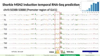
#69 Msn2 is a zinc-finger transcription factor that activates approximately 200 stress-responsive genes by binding to stress-response element motifs in promoter regions.
Under non-stress conditions, Msn2 stays in the cytoplasm
In response to stress signals (for example heat or salt), it translocates into the nucleus.
And binds to stress-response element sites in promoters
#71 Each sequence is 80bp. With adaptors on each side, totaling 110 bps.
#72 Chapter 7 presented Shorkie, a multi-species self-supervised DNA lan- guage model pretrained on a subset of diverse fungal genomes and sub- sequently fine-tuned on TF-induced, time-course yeast RNA-Seq data. By leveraging evolutionary diversity, Shorkie mitigates overfitting in compact S. cerevisiae, accelerates convergence during training, and delivers marked im- provements in both gene-expression and variant-effect prediction on cis-eQTL and MPRA benchmarks.
#75 Conclusion, let’s take a step back to the title of my dissertation—“the language of genomes.”
This idea traces back to Steve Jones’s 1993 book *The Language of Genes*, which offers a nice analogy: codons as words and genes as sentences.
Today, genome language modeling extends that analogy — treating recurring k-mer motifs as tokens, and modelling long-range dependencies as grammatical rules.
#76 For example, if we lay out the splicing gene regulatory patterns alongside grammatical dependencies in natural language, you can see a striking parallel.
Just as words in a sentence influence each other, genomic regions regulate—or are regulated by—other regions.
Our goal is to capture these relationships to decode this underlying grammar of regulation in the genome.
Especially the second half of my thesis, splice site prediction and RNA-Seq coverage prediction.
I hope I've persuaded you that deep learning is a powerful approach to tackle this challenge.
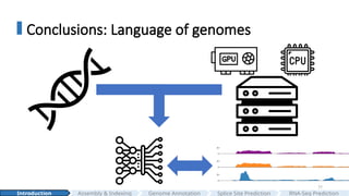
#77 Advances in long-read sequencing technologies and improved algorithms have made gapless, reference quality assemblies routine. [CLICK]
Now we have more genomes, more accurate annotations, and much more computation power which allow us to build large-scale DNA deep learning models.
[CLICK]
Fine-tuned with time-course multi-omics data, these models are able to predict gene expression at base-pair resolution, predict variant effects, and even link regulators to their targets to build the regulatory network.
This thesis lays the methodological foundation for the vision —
By bridging experimental sequencing data with scalable algorithms and AI, I believe that, in the near future, the genomics community will move beyond static reference genomes toward more dynamic, predictive models that help us better understand the language of genome.
#78 First, my sincere thanks to my committee for your guidance and service.
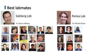
To my PhD advisors, Steven Salzberg and Mihaela Pertea: thank you for visionary mentorship, trust, and encouragement. You gave me the freedom to explore genomics and deep learning and supported my work on Han1, LiftOn, Splam, and OpenSpliceAI. I owe you both an immense debt of gratitude. Thank you for your mentorship over the past four years.
I’m equally grateful to Dr. Ben Langmead for guidance on my WGT qualifying project and for foundations in genomics, sketching, and indexing that shaped how I think.
My heartfelt thanks to Dr. David Kelley, for hosting my 2024 Calico internship and entrusting me with Shorkie project—your mentorship changed my career trajectory.
I’m also grateful to Dr. Anqi Liu—your ML course sparked Splam idea, and your insights strengthened OpenSpliceAI project.
#79 To the all the members in Salzberg and Pertea labs: thank you for your collaboration, camaraderie, curiosity, friendship, and for always pushing science to new heights together.
#80 To the communities at CCB, Computer Science, and Biomedical Engineering: you made Baltimore feel like home.
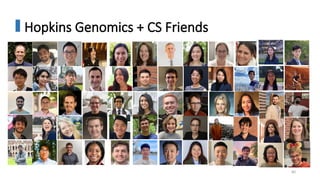
Four years ago, I came to the US alone, starting a new chapter of my life without knowing anyone. Four years later, I have been fortunate to meet all of you—amazing friends, colleagues, and mentors at Hopkins. You are truly incredible.
#81 We had many great memories,
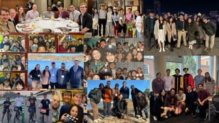
Conference gala, Halloween parties, BDP Science Center party, CS holiday party, more parties, ISMB, RECOMB, Cold Spring Harbor conference memories.
We cheered one another on throughout our growth and celebrated our journeys toward a bright future.
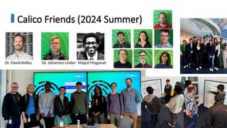
#82 My heartfelt thanks to David Kelley, Johannes Linder, majed magzoub, and all the Kelley lab members for welcoming me during my 2024 Calico internship and trusting me with the Shorkie project. Your mentorship showed me the power of deep learning in genomics and profoundly shaped my career trajectory. I could not be more grateful for the opportunity and guidance you provided.
#83 To friends in Baltimore: Jenny, Nicole, Jakson, Zongyung, Yuyu, Abo, 庚成, Erica, Joy, Billy, Dorian, Pat, Natalie, Trung, Yeongseo, and many more—thank you for the laughter and support. You all makes Baltimore feel like home.
To my close gym buddies—Bobby, Richard, and Jay—thanks for the early mornings, encouragement, and for always bringing out the best in me.
#84 To my friends from Taipei Municipal Chien Kuo High School—鈺能, 柏翰, 維揚, 洸程, and many others—thank you for more than a decade of friendship; you’ve been a constant in my life.
To my college friends 謙熠, 其叡, 斯嘉, 培威, 鄭欣, and others—thank you for your kindness and support. I’m grateful we met during those fearless, dream-chasing years; you pushed me to become a better person.
#85 This is one of my favorite slides.
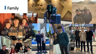
To my basketball family, Team GenoMalone—Bowen, Celine, Mahler, Gus, Erik, Nate, Richard, Bobby—and to my Taiwanese hoop crew Tiger, Leon, Feng-Chiao, Ernie : thanks for the heart, hustle, and friendship you bring on and off the court. And for reminding me that balance and play are as important as work. Our quarterfinal run was a great step; next time, let’s bring home the championship.
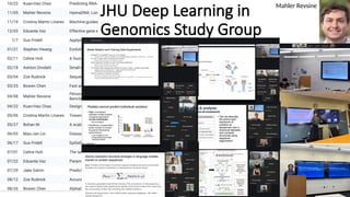
#86 A special shout-out to Mahler, my partner in co-founding the JHU Deep Learning in Genomics Study Group—and to every student who volunteered and joined the discussions.
This study group could not happen without you.
Thank you all for building this community with me, and I believe it will keep inspiring future Hopkins researchers.
#87 To my girlfriend, Pei-Ju Chiang: Your steadfast support, endless encouragement, and gentle wisdom have lifted me through
every high and carried me through every low. Thank you for being my anchor,
my confidante, and the brightest light in my life.
Finally, to my parents and my younger brother, although you have no ideas what I am working on, but your unlimited love, unflagging faith, and countless sacrifices have paved every step of my journey. Your belief in me has been the guiding star that led me to pursue my dream of becoming a scientist.
#88 I’m grateful to the many mentors who shaped my path: 劉玉山 at 建國中學, who sparked my love of biology; Eric Chuang and Tzu-Pin Lu at National Taiwan University; Robert Lanfear at the Australian National University, who introduced me to phylogenetics; Huai-Kuang Tsai at Academia Sinica; and the generous mentors at Hopkins and Calico mentioned earlier. Your guidance, patience, and belief in me made all the difference. I’m deeply thankful.
#89 Next, I’m excited to join Illumina AI Lab as a Senior Deep Learning Scientist. Thank you all for shaping me into the scientist and person I am today

![38
𝑊 =5000𝐹=10,000
𝐿=33200
𝐿=14600
𝐿=25000
Gene 1
Gene 2
Gene n
…
Raw gene DNA sequence
[7, 15000, 4]
[3, 15000, 4]
[5, 15000, 4]
[7, 5000, 3]
[3, 5000, 3]
[5, 5000, 3]
X Y
…
~20k protein-coding genes
Assembly & Indexing
Introduction Genome Annotation Splice Site Prediction RNA-Seq Prediction](https://image.slidesharecdn.com/0825defensepublic-250905174514-7ab4fcd7/85/Kua-Hao-Chao-s-Doctoral-Dissertation-Defense-Slides-38-320.jpg)


![Polymer [ बहुलक ] Chemistry Notes PDF - Irfanullah Mehar - JJ Sir Chemistry.pdf](https://cdn.slidesharecdn.com/ss_thumbnails/polymerchemistrynotespdf-irfanullahmehar-jjsirchemistry-260210172118-3f9b37f7-thumbnail.jpg?width=640&height=640&fit=bounds)


