jacobi method with example

1. PRESENTATION MATLAB
Sajjad Ahmad
2015-CH-241

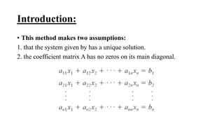
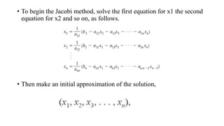
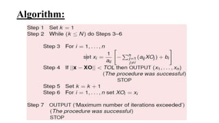
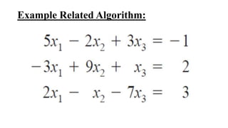
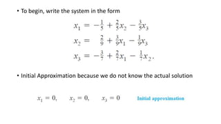
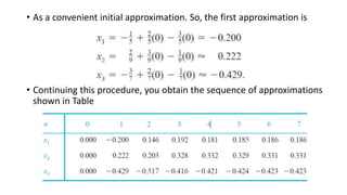
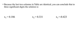
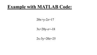
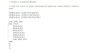
2. Contents:
• Introduction of Jacobi Method
• Algorithm
• Example related algorithm
• Code for Jacobi Method
• Example with code
• Applications in Engineering
• Advantages and Disadvantages

3. Introduction:
• This method makes two assumptions:
1. that the system given by has a unique solution.
2. the coefficient matrix A has no zeros on its main diagonal.

4. • To begin the Jacobi method, solve the first equation for x1 the second
equation for x2 and so on, as follows.
• Then make an initial approximation of the solution,

5. Algorithm:

6. Example Related Algorithm:

7. • To begin, write the system in the form
• Initial Approximation because we do not know the actual solution

8. • As a convenient initial approximation. So, the first approximation is
• Continuing this procedure, you obtain the sequence of approximations
shown in Table

9. • Because the last two columns in Table are identical, you can conclude that to
three significant digits the solution is:
x1 = 0.186 x2 = 0.331 x3 =-0.423

10. Matlab Implementation for jacobi method:

11. Example with MATLAB Code:
20x+y-2z=17
3x+20y-z=-18
2x-3y+20z=25

13. Applications in Engineering:
• Efficient methods of solving systems of linear equations, especially when
approximate solutions are already known.
• Significantly reduce the amount of computation required.
• Plotting and analyzing mathematical relationships(2D and 3D)
• List and matrix operations
• Symbolic manipulation of equations
• Composition analysis of a distillation column system
• Temperature analysis for thermodynamics state equations

14. Advantages
• Fully diagonalizes a
symmetric matrix in one
iteration
• Easy to program
• Stable.
Disadvantages
• Works only for symmetric
matrices (but this is what
one needs for SVD)
• Slow

15. Little Thing is Big Thing