introduction-brownian-motion final

An Introduction to Brownian Motion
Kimthanh Nguyen
May 19, 2016
1 Introduction
Brownian motion is the jittery movement observed in 2 dimensions under a microscope when parti-
cles bounce around in 3 dimensions. Originally discovered by a biologist, Robert Brown, Brownian
motion is modeled as a stochastic process. This is also called a Wiener process with the operator
1
2∆.
For this paper, I will start with a one-dimensional discrete Brownian motion, motivated by the
story of a drunk trying to find his way home. Using the analogue of the drunk and his quest home
walking in a straight line (and his expected probability of making it back home), I explore important
characteristics of Brownian motion: (1) that it is a memory-less process (also known as Markov), (2)
that it is homogeneous in regards to time and space, and finally, (3) by taking the limit of discrete
steps of the drunk, we get continuous Brownian motion of a particle.
After the one-dimensional case, I will explore the symmetric n-dimensional case leading to a
unique solution. Starting with a more realistic drunk, I once again discover his expected probability
of making it home. This is accomplished using lattice and point coordinate remodeling. Then, by
taking the limit of the discrete steps, I will get to particle diffusion and solve using the Brownian
motion partial differential equation and its initial condition. The progression follows Salsa’s Chapter
2: Diffusion in his book Partial Differential Equations in Action [4].
2 History
In 1827, Robert Brown, a biologist, noticed unusual "motions" of particles inside of pollen grains
under his microscope. The pollen grains were suspended in water and had a jittery movement.
He attributed this motion to "being alive." The actual cause for this motion is water molecules.
While undergoing thermal motion, water molecules bombard the pollen particles, creating Brownian
motion [5].
In 1905, Albert Einstein solved the Brownian motion puzzle through modeling the movements
of "bodies of microscopically-visible size" suspended in a liquid using the molecular kinetic theory
of heat. He found that these movements can be accounted for by the molecular motions of heat [2].
In 1923, Norbert Wiener proved the existence of Brownian motion by combining measure theory
and harmonic analysis to find an equation that fulfills all of Einstein’s criteria for Brownian motion
constraints and properties [3].
In 1939, Paul Levy proved that if the normal distribution is replaced by any other distribution in
Einstein’s criteria then either no stochastic process exists or that it is not continuous [3]. Following
1

Levy, many developments were made by Ito and Donsker that facilitate the application of stochastic
process to finance and other areas.
3 Symmetric One-Dimensional Discrete Brownian Motion
3.1 Motivation: To Save a Drunk
Consider a one-dimensional drunk who is leaving the Red Herring, modeled as point x = 0 on a
one-dimensional straight path back to his home in Morgan. During an interval of time τ he can
take one step of length h. Because he is very drunk, he has a p = 1
2 probability of stepping to the
left or right. Let his room in Morgan be point x on the same axis. What is the probability that the
poor drunk would make it back to Morgan at time t?
3.2 Mathematical Model
Model the drunk as a unit mass particle that moves randomly along the x axis with fixed h > 0
space step and τ > 0 time step. During any interval τ, the particle takes one step of unit length h
starting at x = 0. It moves to the left or right with probability 1
2 in a memory-less process, meaning
that any step is done independently of previous steps.
At time t = Nτ, the drunk has taken N steps where N ≥ 0, and ends up at some point x = mh
where −N ≤ m ≤ N. Of course, both N and m are integers, since we are only modeling discrete
steps. Our goal is to find p(x, t), or the probability of finding the particle at point x at time t.
3.3 Computation of p(x,t)
Let x = mh be the position of the drunk after N steps. To reach this position x the drunk has
already walked k steps to the right and N − k steps to the left, with 0 ≤ k ≤ N, then:
m = k − (N − k) = 2k − N
since each left step cancels each right step perfectly, leaving the position mh be the difference
between the number of left and right steps taken up until time t. From the expression above we also
see that either both m and N are even or both m and N are odd integers. Rearranging, we have:
k =
1
2
(N + m)
Thus
p(x, t) = pk =
number of walks with k steps to the right given the drunk has already taken N steps
number of possible walks from taking N steps
because of the relationship between k, N, and m.
pk =
N
k
2N
=
N!
k!(N−k)!
2N
x = mh, t = Nτ, k =
1
2
(N + m)
since N
k is the number of possible walks with k steps to the right and N − k steps to the left and
2N is the number of possible paths for N steps (each step chosen doubles the number of paths).
2

The mean displacement of x after N steps, or the expected value of m after N steps, or
the first moment of x after N steps, is denoted as x = m h. The second moment of x after N
steps is denoted as x2 = m2 h2. The variance of x is var(x) = x2 − x 2
.
The average distance from the origin after N steps, or the standard deviation of x, is x2 − x 2
,
which can be approximated by the quantity x2 = m2 h. This is because x = 0, a fact that
we will later prove.
Because m = 2k − N, we have:
m = 2 k − N
which when squared leads to the following result:
m2
= 4 k2
− 4 k N + N2
Therefore, we only need to compute k and k2 to get to m and m2 . We know that pk =
(N
k )
2N ,
which means:
k =
N
k=1
kpk =
1
2N
N
k=1
k
N
k
, k2
=
N
k=1
k2
pk =
1
2N
N
k=1
k2 N
k
While it is possible to calculate k and k2 directly from above, from probability, we can use
moment generating function to find the first and second moments of k:
G(s) =
N
k=0
pksk
=
1
2N
N
k=0
N
k
sk
Taking the derivative of the moment generating function, we have:
G (s) =
N
k=1
kpksk−1
, G”(s) =
1
2N
N
k=2
k(k − 1)
N
k
sk−2
Letting s = 1, we can see that:
G (1) =
N
k=1
kpk = k , G (1) =
1
2N
N
k=2
k(k − 1)
N
k
= k(k − 1) = k2
− k
which are the expected value of k and a way to get the second moment of k.
Letting a = 1 and b = s in the binomial formula:
(a + b)N
=
N
k=0
N
k
aN−k
bk
We know that the moment generating function is:
G(s) =
1
2N
(1 + s)N
which implies:
G (1) =
N
2
= k and G (1) =
N(N − 1)
4
3

Using k and G (1), we solve to get:
k2
=
N(N + 1)
4
Because m = 2k − N,
m = 2 k − N = 2
N
2
− N = 0 = x
which makes sense because there is symmetry in the random walk.
m2
= 4 k2
− 4 k N + N2
= 4
N(N + 1)
4
− 4
N
2
N + N2
= N2
+ N − 2N2
+ N2
= N
which from our earlier expression x2 = m2 h means the standard deviation of x is:
x2 =
√
Nh
The standard deviation suggests that, at time Nτ, the distance from the origin is of order
√
NH,
which means that the order of the time scale is the square of the space scale. In order to preserve
the standard deviation of x in the limit process, we must use a space-time parabolic dilation (rescale
the time as the square of the space).
With this information in mind, we are going to set up a difference equation to carry out the
limit procedure for the transition probability p = p(x, t).
3.4 The Limit Transition Probability
Recall one of the characteristics of the drunk: he doesn’t have any memory of his last step, and
each move is independent from the previous one. Therefore, if his position is x at time t + τ, at
time t, his previous position has to be x − h or x + h. Putting this into a total probability formula,
we have:
p(x, t + τ) =
1
2
p(x − h, t) +
1
2
p(x + h, t)
with initial conditions p(0, 0) = 1 and p(x, 0) = 0 if x = 0.
Fixing x and t, we can examine what happens when h → 0, τ → 0. Essentially this is looking
at smaller and smaller steps in smaller and smaller time spans until we can get to the continuous
case. We can think of p as a smooth function defined in the whole half plane R × (0, +∞) and not
only at the discrete set of points (mh, Nτ), which is what the discrete steps previously gave us. By
passing to the limit, we will find a continuous probability distribution so that p(x, t), which is the
probability of finding the drunk at (x, t), is zero. If we interpret p as a probability density then this
inconvenience disappears. Using Taylor’s formula/approximation we can write this:
p(x, t + τ) = p(x, t) + pt(x, t)τ + o(τ)
p(x + h, t) = p(x, t) + px(x, t)h +
1
2
pxx(x, t)h2
+ o(h2
)
p(x − h, t) = p(x, t) − px(x, t)h +
1
2
pxx(x, t)h2
+ o(h2
)
4

Substituting this into the original equation p(x, t + τ) = 1
2p(x − h, t) + 1
2p(x + h, t), we have:
p(x, t+τ) =
1
2
p(x, t)−px(x, t)h+
1
2
pxx(x, t)h2
+o(h2
) +
1
2
p(x, t)+px(x, t)h+
1
2
pxx(x, t)h2
+o(h2
)
Simplifying the algebra explicitly further, we get:
p(x, t + τ) = p(x, t) +
1
2
pxx(x, t)h2
+ o(h2
)
Plugging in p(x, t) + pt(x, t)τ + o(τ) = p(x, t + τ), once again we get this explicit expression:
p(x, t) + pt(x, t)τ + o(τ) = p(x, t) +
1
2
pxx(x, t)h2
+ o(h2
)
Subtracting p(x, t) from both sides, we have:
ptτ + o(τ) =
1
2
pxxh2
+ o(h2
)
Dividing by τ:
pt + o(1) =
1
2
pxx
h2
τ
+ o(
h2
τ
)
In order for us to obtain something non-trivial, we need to require that h2
τ has to have a finite and
positive limit. The simplest choice is to have:
h2
τ
= 2D
for some D > 0. Passing through the limit:
pt = Dpxx
∂p
∂t
= D
∂2p
∂x2
And the initial condition becomes:
lim
t→0+
p(x, t) = δ0
Where δ0 is a delta spike at 0. That is, we are requiring that the probability of the particle being
at x = 0 at t → 0 is 1 (and that the probability of it being at x = 0 is 0).
We define Fourier transform as a linear operator mapping a function f(x), x ∈ R, to a function
ˆf(k), k ∈ R such that:
[F][f](k) = ˆf(k) :=
1
√
2π
∞
−∞
e−ikx
f(x)dx
We define the inverse Fourier transform as a linear operator mapping a Fourier transformed
function ˆf(k), k ∈ R back to a function f(x), x ∈ R such that:
[F−1
][ ˆf](k) = ˆf(k) :=
1
√
2π
∞
−∞
eikx ˆf(x)dx = f(x)
5

Taking inverse Fourier transform of the Fourier transform of p(x, t) with respect to x, we have:
p(x, t) =
1
√
2π
∞
−∞
eikx
ˆp(k, t)dx
Differentiating both sides with respect to x, we have:
px(x, t) =
1
√
2π
∞
−∞
ikeikx
ˆp(k, t)dx = F−
1[ikˆp]
Differentiating both sides with respect to x again, we have:
pxx(x, t) =
1
√
2π
∞
−∞
(ik)2
eikx
ˆp(k, t)dx = F−
1[−k2
ˆp]
Taking inverse Fourier transform of the Fourier transform of pt(x, t) with respect to x, we have:
pt(x, t) =
1
√
2π
∞
−∞
eikx
ˆpt(k, t)dx = F−1
[ˆpt]
Plugging these three equations into the original partial differential equations, we have:
ˆpt(k, t) = −k2
Dˆp(k, t), ˆp(k, 0) = ˆδ0 = 1
This is an ODE of t with k ∈ R treated as a parameter. The solution is:
ˆp(k, t) = e−k2Dt
[1]
To return to p(x, t) we apply the inverse Fourier transform:
p(x, t) =
1
√
2π
∞
−∞
eikx
e−k2Dt
dk
Let a = Dt, we can rewrite the inverse Fourier transform of the Gaussian as:
p(x, t) = F−1
[e−ak2
]
=
1
√
4πa
e
−x2
4a [6]
=
1
√
4πDt
e− x2
4Dt
This fundamental solution is also the solution to the diffusion problem:
p(x, t) =
1
√
4πDt
e− x2
4Dt = ΓD(x, t)
D is the diffusion coefficient. We know that:
h2
=
x2
N
, τ =
t
N
6

h2
τ
=
x2
t
= 2D
This means that in unit time, the particle diffuses an average distance of
√
2D. We also know that
the dimension of D are [length]2 ∗ [time]−1, which means that x2
Dt is also dimensionless, not only
just invariant by parabolic dilation. We can also deduce from h2
τ = 2D that:
h
τ
=
2D
h
→ +∞
which means that the average speed h
τ of the particle at each step becomes unbounded. Therefore,
the fact that the particle diffuses in unit time to a finite average distance is purely due to the rapid
fluctuations of the motion.
3.5 To Brownian Motion
In order to find out what happens to random walks in the limit, we need to get help from probability.
Let xj = x(jτ) be the position of an infinitely small drunk after j steps for j ≤ 1, let:
hξj = xj − xj−1
for ξj independently identically distributed random variables. Each ξj takes on a value 1 or -1
with probability 1
2. Their expectation is ξj = 0 and their variance is ξ2
j = 1. The drunk’s
displacement after N steps is:
xN = h
N
j=1
ξj
Let h = 2Dt
N , which means h2
τ = 2D, and let N → ∞, by the Central Limit Theorem, we
know that xN coverges to a random variable X = X(t) that is normally distributed with mean 0
and variance 2Dt with density ΓD(x, t). This means that the discrete random walk has become a
continuous walk as the drunk’s step size and step time shrink smaller and smaller at the limit. If
D=1
2 it is called a 1 dimensional Brownian motion or Wiener process.
We denote the random position of the infinitely small drunk by the symbol B = B(t), called the
position of the Brownian particle. The family of the random variable B(t) where t plays the role
of a parameter is defined on a common probability space (Ω, F, ρ) where Ω is the set of elementary
events, F is a σ-algebra in Ω of measurable events, and ρ is a suitable probability measure in F. The
right notation is B(t, ω) where ω ∈ Ω but the dependence on ω is often omitted and understood.
The family of B(t, ω) is a continuous stochastic process. Keeping ω ∈ Ω fixed, the random
variable ω ∈ Ω fixed, we get the real function t → B(t, ω) whose graph describes a Brownian path.
Keeping t fixed, we get the random variable ω → B(t, ω).
Without caring too much of what really is ω, it is important to be able to compute the probability
P{B(t) ∈ I} where I ⊆ R is a reasonable subset of R.
We can summarize everything in this formula:
dB ∼
√
dtN(0, 1) = N(0, dt)
where X ∼ N(µ, σ2) is the normal distribution with mean µ and standard deviation σ.
Here are some characteristics of Brownian motion:
7

• Path continuity:
With probability 1, the possible paths of a Brownian particle are continuous functions: t →
B(t), t ≥ 0. Because the instantaneous speed of the particle is infinite, their graphs are
nowhere differentiable.
• Gaussian law for increments:
We can allow the particle to start from a point x = 0 by considering the process Bx(t) =
x+B(t). With every point x, there is an associated probability Px with the following properties
if x = 0 and P0 = P:
1. Px{Bx(0) = x} = P{B(0) = 0} = 1
2. For every s ≥ 0, t ≥ 0, the increment Bx(t+s)−Bx(s) = B(t+s)−B(s) follows normal
law with zero mean and variance t with density Γ(x, t) = Γ1
2
(x, t) = 1√
2πt
e
−x2
2t . It is also
independent of any event occurred at a time ≤ s. This means that two events
{Bx
(t2) − Bx
(t1) ∈ I2} {Bx
(t1) − Bx
(t0) ∈ I1}, t0 < t1 < t2
are independent.
• Transition probability:
For each set I ⊆ R, a transition function P(x, t, I) = Px{Bx(t) ∈ I} is defined as the
probability of the particle that started at x to be in the interval I at time t. We can write:
P(x, t, I) = P{B(t) ∈ I − x} =
I−x
Γ(y, t)dy =
I
Γ(y − x, t)dy
• Invariance: The motion is invariant with respect to translations.
• Markov and Strong Markov properties:
Let µ be a probability measure on R, if the initial position of a particle is random with a
probability distribution µ, then we can write the Brownian motion with initial distribution
µ as Bµ. This motion is associated with a probability distribution Pµ such that for every
reasonable set F ⊆ R, Pµ{Bµ(0) ∈ F} = µ(F).
We can find the probability that the particle hits a point in I at time t with:
Pµ
{Bµ
(t) ∈ I} =
R
Px
{Bx
(t) ∈ I}dµ(x) =
R
P(x, t, I)dµ(x)
The Markov property states that given any condition H, related to the behavior of the particle
before time s ≥ 0, the process Y (t) = Bx(t+s) is a Brownian motion with initial distribution
µ(I) = Px{Bx(s) ∈ I|H}. Having this property means that future process Bx(t + s) is
independent from the past and the present process Bx(s).
The strong Markov property states that s is substituted by a random time τ, depending only
on the behavior of the particle in the interval [0, t]. In other words, to decide whether or not
the event {τ ≤ t} is true, it is enough to know the behavior of the particle up to time t.
8

• Expectation:
Given a sufficiently smooth function g = g(y), y ∈ R, we can define the random variable
Z(t) = (g ◦ Bx)(t) = g(Bx(t))
. The expected value is:
Ex
[Z(t)] =
R
g(y)P(x, t, dy) =
R
g(y)Γ(y − x, t)dy
4 Symmetric n-Dimensional Brownian Motion
4.1 Ode to a More Realistic Drunk
Of course, n = 1 is an overly simplified situation for drunks, as any freshman who had to take their
friends back home after First Fridays can vouch. I will go through the same analysis for the n=1
case and extends it to n-dimensional Brownian motion.
4.2 Remodeling
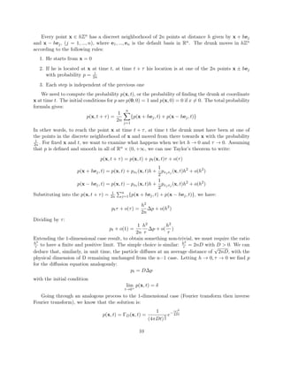
In order to extend the notion of motion, we need to introduce the notion of a lattice Zn given the
set of points x ∈ Rn. Think of x as a vector with signed integer coordinates. Given the space step
h>0, hZn denotes the lattice of points whose coordinates are signed integers multiplied by h.
Figure 1: 2D random walk represented using lattice of points. Source: Page 59, Salsa’s "Partial
Differential Equations in Action"
9

Every point x ∈ hZn has a discreet neighborhood of 2n points at distance h given by x + hej
and x − hej, (j = 1, ..., n), where e1, ..., en is the default basis in Rn. The drunk moves in hZn
according to the following rules:
1. He starts from x = 0
2. If he is located at x at time t, at time t + τ his location is at one of the 2n points x ± hej
with probability p = 1
2n
3. Each step is independent of the previous one
We need to compute the probability p(x, t), or the probability of finding the drunk at coordinate
x at time t. The initial conditions for p are p(0, 0) = 1 and p(x, 0) = 0 if x = 0. The total probability
formula gives:
p(x, t + τ) =
1
2n
n
j=1
{p(x + hej, t) + p(x − hej, t)}
In other words, to reach the point x at time t + τ, at time t the drunk must have been at one of
the points in the discrete neighborhood of x and moved from there towards x with the probability
1
2n. For fixed x and t, we want to examine what happens when we let h → 0 and τ → 0. Assuming
that p is defined and smooth in all of Rn × (0, +∞, we can use Taylor’s theorem to write:
p(x, t + τ) = p(x, t) + pt(x, t)τ + o(τ)
p(x + hej, t) = p(x, t) + pxt (x, t)h +
1
2
pxjxj (x, t)h2
+ o(h2
)
p(x − hej, t) = p(x, t) − pxt (x, t)h +
1
2
pxjxj (x, t)h2
+ o(h2
)
Substituting into the p(x, t + τ) = 1
2n
n
j=1{p(x + hej, t) + p(x − hej, t)}, we have:
ptτ + o(τ) =
h2
2n
∆p + o(h2
)
Dividing by τ:
pt + o(1) =
1
2n
h2
τ
∆p + o(
h2
τ
)
Extending the 1-dimensional case result, to obtain something non-trivial, we must require the ratio
h2
τ to have a finite and positive limit. The simple choice is similar: h2
τ = 2nD with D > 0. We can
deduce that, similarly, in unit time, the particle diffuses at an average distance of
√
2nD, with the
physical dimension of D remaining unchanged from the n=1 case. Letting h → 0, τ → 0 we find p
for the diffusion equation analogously:
pt = D∆p
with the initial condition
lim
t→0+
p(x, t) = δ
Going through an analogous process to the 1-dimensional case (Fourier transform then inverse
Fourier transform), we know that the solution is:
p(x, t) = ΓD(x, t) =
1
(4πDt)
n
2
e−
|x|2
4Dt
10

with Rn p(x,t) dx=1.
Similar to the one-dimensional case, the n-dimensional random walk also became a continuous
walk. When D = 1
2, we can model the n-dimensional Brownian motion as a family of B(t) =
B(t, ω) on a probability space (Ω, F, P). The family of random variables B(t, ω) is a vector valued
continuous stochastic process. For fixed ω ∈ Ω, the vector function t → B(t, ω) describes an
n-dimensional Brownian path. This path has analogous features to the 1-dimensional case:
• Path continuity:
With probability 1, the possible paths of a Brownian particle are continuous functions: t →
B(t), t ≥ 0.
• Gaussian law for increments:
We can allow the particle to start from a point x = 0 by considering the process Bx
(t) =
x + B(t). With every point x, there is an associated probability Px with the following
properties if x = 0 and P0 = P:
1. Px{Bx
(0) = x} = P{B(0) = 0} = 1
2. For every s ≥ 0, t ≥ 0, the increment Bx
(t+s)−Bx
(s) = B(t+s)−B(s) follows normal
law with zero mean and variance tIn with density Γ(x, t) = Γ1
2
(x, t) = 1
(2πt)
n
2
−x2
2t
. It is
also independent of any event occurred at a time ≤ s. This means that two events
{B(t2) − B(t1) ∈ A1} {B(t1) − B(t0) ∈ A2}, t0 < t1 < t2
are independent.
• Transition probability:
For each set A ⊆ Rn, a transition function P(x, t, A) = Px{Bx
(t) ∈ A} is defined as the
probability of the particle that started at x to be in the set A at time t. We can write:
P(x, t, A) = P{B(t) ∈ A − x} =
A−x
Γ(y, t)dy =
A
Γ(y − x, t)dy
• Invariance: The motion is invariant with respect to translations and rotations.
• Markov and Strong Markov properties:
Let µ be a probability measure on Rn, if the initial position of a particle is random with a
probability distribution µ, then we can write the Brownian motion with initial distribution
µ as Bµ
. This motion is associated with a probability distribution Pµ such that for every
reasonable set A ⊆ Rn, Pµ{Bµ
(0) ∈ A} = µ(A).
We can find the probability that the particle hits a point in A at time t with:
Pµ
{Bµ
(t) ∈ A} =
Rn
P(x, t, A)µ(dx)
The Markov property states that given any condition H, related to the behavior of the particle
before time s ≥ 0, the process Y(t) = Bx
(t+s) is a Brownian motion with initial distribution
11

µ(A) = Px{Bx
(s) ∈ A|H}. Having this property means that future process Bx
(t + s) is
independent from the past and the present process Bx
(s).
The strong Markov property states that s is substituted by a random time τ, depending only
on the behavior of the particle in the interval [0, t]. In other words, to decide whether or not
the event {τ ≤ t} is true, it is enough to know the behavior of the particle up to time t.
• Expectation:
Given a sufficiently smooth function g = g(y), y ∈ Rn, we can define the random variable
Z(t) = (g ◦ Bx
)(t) = g(Bx
(t))
. The expected value is:
E[Z(t)] =
Rn
g(y)P(x, t, dy) =
Rn
g(y)Γ(y − x, t)dy
References
[1] P.C. Bressloff. “Chapter 2 Diffusion in Cells: Random Walks and Brownian Motion”. In: Stochas-
tic Processes in Cell Biology, Switzerland: Springer International Publishing, 2014. url: http:
//www.springer.com/cda/content/document/cda_downloaddocument/9783319084879-
c1.pdf?SGWID=0-0-45-1490968-p176811738.
[2] Albert Einstein. “Investigations on the Theory of the Brownian Movement”. In: (1965). url:
http://www.maths.usyd.edu.au/u/UG/SM/MATH3075/r/Einstein_1905.pdf.
[3] Davar Khoshnevisan. The University of Utah Research Experience for Undergraduates Summer
2002 Lecture Notes. Department of Mathematics: University of Utah, 2002. url: http://www.
math.utah.edu/~davar/REU-2002/notes/all-notes.pdf.
[4] Sandro Salsa. Partial Differential Equations in Action: From Modelling to Theory. English. 1st
ed. 2008. Corr. 2nd printing 2010 edition. Milan: Springer, Jan. 2010. isbn: 978-88-470-0751-2.
[5] Karl Sigman. IEOR 4700: Notes on Brownian Motion. 2006. url: http://www.columbia.
edu/~ks20/FE-Notes/4700-07-Notes-BM.pdf.
[6] Eric W. Weisstein. Fourier Transform–Gaussian. en. Text. url: http://mathworld.wolfram.
com/FourierTransformGaussian.html.
12

introduction-brownian-motion final

More Related Content

What's hot

Viewers also liked

Similar to introduction-brownian-motion final

introduction-brownian-motion final