Download as PDF, PPTX
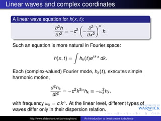
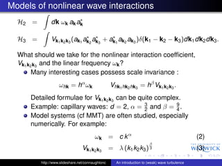
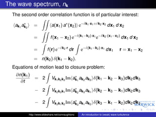
![Conservation laws in turbulence
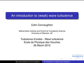
In turbulent systems, quantities which are conserved by the
nonlinear terms in the equations of motion are very important.
Navier-Stokes turbulence
∂v
+ (v · )v = − p + ν∆v + f
∂t
·v=0
1
Nonlinear terms conserve kinetic energy, 2 v2 . Energy is
added by forcing and removed by the viscous terms.
Wave turbulence
∂ak δH
= i ∗ + fk + D [ak ]
∂t δak
In WT, H, is conserved by nonlinearity - not quadratic.
Possibly other conserved quantities (cf Nazarenko lecture).
http://www.slideshare.net/connaughtonc An introduction to (weak) wave turbulence](https://image.slidesharecdn.com/leshouches-mar2012-120327020734-phpapp02/85/Introduction-to-weak-wave-turbulence-9-320.jpg)
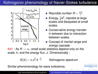
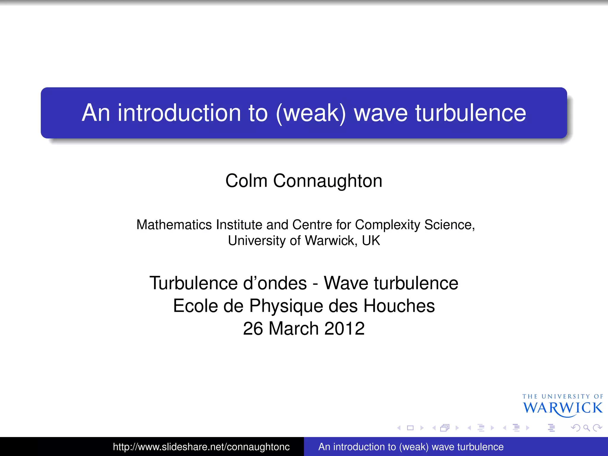
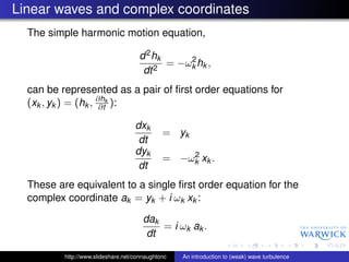
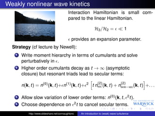
![What can we learn about WT by dimensional analysis?
For the purposes of power counting:
2
H = c k α ak dk + λ k β ak δ(k) (dk)3
3
2
nk δ(k) = ak
Dimensions:
[c] = T −1 K −d
1 1 d
[ak ] = H 2 T 2 K − 2
1 1 d
[λ] = H 2 T 2 K − 2
[nk ] = HT
One more dimensional parameter, the flux:
[J] = HT −1 K d .
Flux is "H per unit volume per unit time".
http://www.slideshare.net/connaughtonc An introduction to (weak) wave turbulence](https://image.slidesharecdn.com/leshouches-mar2012-120327020734-phpapp02/85/Introduction-to-weak-wave-turbulence-11-320.jpg)
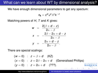
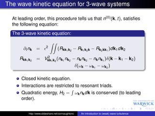
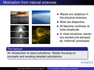
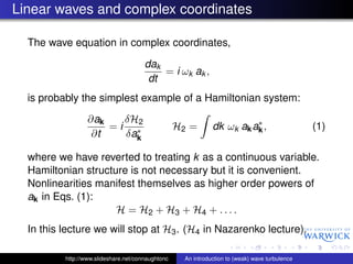
![The wave kinetic equation in frequency space
Details are hidden in the (very messy) kernel L(ω1 , ω2 ). Scaling:
2β − α
L1 (ω1 , ω2 ) ∼ ω ζ , ζ=
α
The frequency-space kinetic equation can be written:
∂Nω
= S1 [Nω ] + S2 [Nω ] + S3 [Nω ].
∂t
The RHS has been split into forward-transfer terms (S1 [Nω ])
and backscatter terms (S2 [Nω ] and S3 [Nω ]).
Each conserves energy independently. S1 [Nω ] describes the
kinetics of cluster aggregation.
http://www.slideshare.net/connaughtonc An introduction to (weak) wave turbulence](https://image.slidesharecdn.com/leshouches-mar2012-120327020734-phpapp02/85/Introduction-to-weak-wave-turbulence-18-320.jpg)
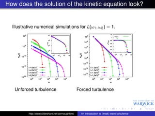
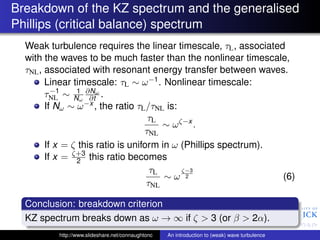
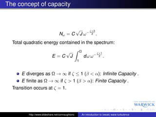
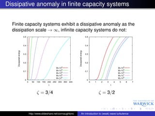

This document provides an introduction to the concept of wave turbulence. It discusses how waves interact nonlinearly at finite amplitudes to produce a statistical, non-equilibrium dynamics. Key points: - Wave turbulence involves dispersive waves that are excited and damped by external processes, leading to interactions between many degrees of freedom. - The nonlinear interactions can be modeled using a Hamiltonian approach by including higher-order terms that couple different Fourier modes. - A central goal is developing a statistical description of the system using correlation functions and obtaining a closed kinetic equation for the wave spectrum. - In the weak turbulence regime, this kinetic equation can be solved perturbatively to obtain scaling laws for the wave spectrum in both physical and


![[Vvedensky d.] group_theory,_problems_and_solution(book_fi.org)](https://cdn.slidesharecdn.com/ss_thumbnails/vvedenskyd-grouptheoryproblemsandsolutionbookfi-org-130405071812-phpapp02-thumbnail.jpg?width=640&height=640&fit=bounds)


