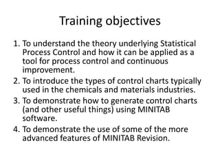
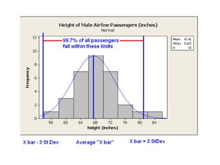
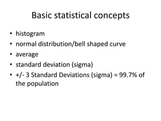
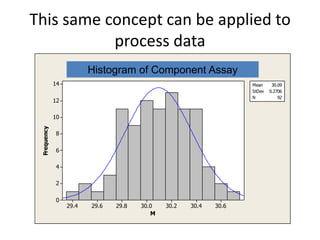
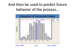
SlideShare a Scribd company logo
1 of 80
Download to read offline
An Introduction to Statistical Process
Control (SPC) and Process Capability
          Estimation (Cpk)
            Robert W. Sherrill
          ASQ Certified Quality Manager
Training objectives
1. To understand the theory underlying Statistical
   Process Control and how it can be applied as a
   tool for process control and continuous
   improvement.
2. To introduce the types of control charts typically
   used in the chemicals and materials industries.
3. To demonstrate how to generate control charts
   (and other useful things) using MINITAB
   software.
4. To demonstrate the use of some of the more
   advanced features of MINITAB Revision.
References
Economic Control of Quality of Manufactured Product
By W.A. Shewhart, PhD , published 1931


Walter Shewhart (1891-1967), PhD Physics,
   Member of the Technical Staff at Bell
   Telephone Laboratories, is generally
   considered the father of Statistical Process
   Control and a major contributor to the
   application of statistics to manufacturing.


He was influential in the development of two
   other major quality leaders of the 20th
   century, W.E. Deming and Joseph Juran.
References
•   Understanding Variation: the Key to Managing Chaos
•   Donald J. Wheeler, Second Edition, published 2000

•   Understanding Statistical Process Control
•   Donald J. Wheeler and David S. Chambers, Second edition, published 1992

•   Advanced Topics in Statistical Process Control
•   Donald J. Wheeler, published 1995

•   Donald J. Wheeler PhD is one of the most understandable of the current
    generation of authors on SPC. His books range from simple explanations of SPC
    (Understanding Variation) to a review of some of the most advanced questions in
    the field (Advanced Topics in Statistical Process Control). His book on
    Measurement Systems Analysis, Evaluating the Measurement Process, is also
    excellent.
References
• Statistical Process Control (SPC) Reference
  Manual
• DaimlerChrysler Corporation, Ford Motor
  Company, and General Motors Corporation,
  Second Edition, Issued July 2005
•   This manual was developed by the U.S. automobile industry and the American Society
    for Quality as an introduction to the SPC as part of the QS 9000 automotive quality
    standard.

•   It is a very practical guide to SPC, and has the added value of being recognized within
    the automobile industry (remember that ISO/TS 16949 is an automobile industry
    quality standard).
References
Articles regarding Non Normal SPC
1. William A. Levinson and Angela M. Polny, “SPC for Tool
   Particle Counts”, Semiconductor International, June 1,
   1999
2. William A. Levinson, “Statistical Process Control for
   Nonnormal Distributions”, www.ct-
   yankee.com/spc/nonnormal.html
3. Thomas Pyzdek, “Non-Normal Distributions in the Real
   World”, Quality Digest, December 1999
4. Robert W. Sherrill and Louis A. Johnson, “Calculated
   Decisions”, Quality Progress, January 2009
A few cautionary notes regarding Statistical Process Control

•    Statistical Process Control is a quality management tool; it is not an exact science.
•    As with any tool, if SPC does not work in the intended application, or if another tool works
     better; then discard it and find another tool that works better. A hammer is a useful tool, but
     you can’t fix everything with a hammer.
•    The field of SPC is full of reference text books, articles, and self declared “experts”. These
     books, articles and experts are often in disagreement with one another.
•    I am not an “expert”. I have attempted to cite the sources of the information included in this
     presentation, and to offer my opinions based on my own understanding of SPC, and my
     experience (20 years and counting) in quality management.
•    I would encourage all of you to trust your own ability to apply this tool to practical problems,
     and to trust your own intuition and common sense.
•    I hope that you will find this presentation useful.

Robert W. Sherrill
ASQ Certified Quality Manager, Certified Quality Engineer, and Certified Six Sigma Black Belt
March 24, 2011
A review of the basics of Process
             Control
What is a process?

 a series of activities linked to perform a specific objective
 has a beginning, an end, and clearly identified inputs and
  outputs
 processes generally cut across organizational boundaries
 has a customer (internal or external)


•   reference: Management Accounting, Ansari, 1997)
Process Control begins with clearly defining the process
               to be used (every time):
                         Collect all parts
                           needed for
                            assembly


                                                   Ask Store Room to
                          Are all parts
                                                    deliver missing
                           present?
                                                         parts


                           Assembly                 Ask Maintenance
                           machine in              to repair Assembly
                          good order?                   Machine


                         Assemble parts


                  Verify parts are good, move to
                 Finished Goods Kanban location
By controlling all process
inputs we can achieve a
process output that is stable
and in control
This chart is formally called a Cause
and Effect diagram.

More often it is called a fishbone
diagram, or the Ishikawa diagram
after its inventor, Dr. Kaoru Ishikawa.

The Inputs “bones” are often referred
to as the 4 M’s and an E.

There are other versions of this
diagram with 5, 6 or even 8 M’s, but
the basic concept is still the same.
But what do we mean by “stable” and
            “in control”?


• First, we have to learn a little about
  “variation” and statistics.

• Exercise -develop a histogram for the height of
  people in class
A simple histogram of heights of male
            airline passengers
 Notice that there is a wide range
  of heights in this sample, but the
  average male passenger is about
  68 inches tall.
                                                              Height (inches) of Male Airline Passengers
 Notice also that the populations                  12


  on either side of the average are                 10


  significant, but not quite as large               8


                                        Frequency
  as the average.                                   6


 If we fitted a smooth curve to the                4

  tops of each of these columns it                  2

  would be rather bell shaped.                      0
                                                         56      60      64     68       72     76    80   84
                                                                              height (inches)
Histogram fitted with Normal
        distribution

                       Height of Male Airline Passengers (inches)
                                          Normal
             12                                                      Mean    67.42
                                                                     StDev   5.657
                                                                     N          33
             10


             8
 Frequency


             6


             4


             2


             0
                  56    60     64      68      72     76   80   84
                                    height (inches)
The Normal distribution has some
     useful characteristics…
Basic statistical concepts
•   histogram
•   normal distribution/bell shaped curve
•   average
•   standard deviation (sigma)
•   +/- 3 Standard Deviations (sigma) = 99.7% of
    the population
This same concept can be applied to
           process data
                  Histogram of Component "M" in an EKC Remover Product
                         Histogram of Component Assay
                                      Normal
             14                                                      Mean     30.09
                                                                     StDev   0.2706
                                                                     N           92
             12

             10
 Frequency


             8

             6

             4

             2

             0
                  29.4   29.6   29.8   30.0   30.2   30.4   30.6
                                          M
And then be used to predict future
    behavior of the process…
      Histogram of Component Assay
X bar +/- 3 Standard Deviations can be used to set
                 Control Limits on a Control Chart


                                          Control Chart for Component Product
                                           Control Chart for Component "M" in a EKC Remover Assay
                                          31.0
                                                                                                        UCL=30.895


                                          30.5
                       Individual Value


                                                                                                        _
                                                                                                        X=30.094
                                          30.0


                                          29.5

                                                                                                        LCL=29.294

                                                 1   10   19   28   37   46    55   64   73   82   91
                                                                     Observation


*Historical note- Dr. Shewhart decided to use three standard deviations to establish control limits because it seemed to work
well in practice. There is no “3 Sigma Law” that requires control limits to be set this way. It just works well!
And then be used to generate a Control Chart that can
         be used to predict future behavior:


        Control Chart for Component Assay
Key concepts of Statistical Process
                 Control

•   Average (mathematical mean)
•   Upper Control Limit
•   Lower Control Limit
•   99.7%
•   Common Causes of Variation
•   Special Causes of Variation
A Control Chart is an excellent tool for
monitoring “stability” and “in control”
Control charts distinguish between “common causes”
 and “assignable causes” of variation.
Charts that stay within their Upper and Lower Control
 Limits are displaying “common causes” of variation
 (due to natural variations in raw materials, equipment,
 environment et cetera).
  – These charts, and the processes that they represent, can be called
    stable and in control
Charts that have many “excursions” above the UCL or
 below the LCL are not stable or in control. There are
 evidently some “special” or “assignable” causes of
 variation that have not been identified or controlled.
Different types of SPC charts


and a little guidance on when to use them
Review of Control Chart
             Assumptions
• In order for control charts to be meaningful,
  the following conditions must apply:
  – Process inputs (4M’s and E) are consistent and not
    likely to change much over time
  – Process output data are normally distributed (i.e.
    fit a bell shaped histogram), or can be modified to
    fit a bell shaped curve
The Individual, Moving Range chart works well with normally
                      distributed data


                                                    I-MR Chart of Component "Q"
                               31.0
                                                                                                      U C L=30.895
        Individual V alue


                               30.5

                                                                                                      _
                                                                                                      X=30.094
                               30.0


                               29.5
                                                                                                      LC L=29.294
                                      1   10   19   28    37        46       55   64   73   82   91
                                                               O bser vation

                                          1
                                1.2

                                                                                                      U C L=0.983
               M oving Range


                                0.9


                                0.6

                                                                                                      __
                                0.3                                                                   M R=0.301


                                0.0                                                                   LC L=0
                                      1   10   19   28    37        46       55   64   73   82   91
                                                               O bser vation
Individual, Moving Range Charts
•   Generally used when dealing with large, homogeneous batches of product or
    continuous measurements.

     – Within-batch variation is much smaller than between-batch variation.
     – Range charts are used in conjunction with Individual charts to help monitor dispersion*.

•   I, MR charts are not recommended if the data are not normally distributed.


     *Per Thomas Pyzdek, “there is considerable debate over the value of moving R charts. Academic researchers have failed to
         show statistical value in them. However, many practitioners (including the author) believe that moving R charts
         provide value additional information that can be used in trouble shooting)”. Reference The Complete Guide to the
         CQE. See also Wheeler, Advanced Topics in SPC, page 110.
What happens if the assumptions
          do not apply
• If the inputs (4M’s and an E) are not stable
  and (relatively) well controlled, work with
  your suppliers, equipment engineers and
  manufacturing people to stabilize the process.
  – A simple run chart may be useful during this
    process improvement effort
Alright, I’ve done that, but the
    histogram still looks funny…
• If you have already worked to control the 4m’s
  and an E and the output data still look
  “funny”, then there are techniques that can be
  applied to make the data look “normal”.
One solution is to try a data transformation
     Process data histograms that look like this:   Can be made to look like this by
                                                        transforming the data:


Common transformations include taking the square root , log, natural log, or exponential of the
   data and treating that as the variable. I have not found this technique to be very useful,
   because the control limits are expressed in terms of the transformed number, not the “real”
   number.
Another solution that works well for those of you dealing with randomly
 selected samples is to work with averages and ranges
The average values of randomly selected   Will tend to be normally distributed when plotted
samples from any distribution…            on a histogram.


                                              This phenomenon is explained by
                                              something called the Central Limit
                                              Theorem and is easily tested by taking any
                                              data set, randomly pulling samples,
                                              measuring them, calculating the average
                                              values, and plotting the results on a
                                              histogram.
Example of an X-bar, R chart


                               An important
                               thing to note on
                               these dual
                               charts is that
                               both charts
                               have to be in
                               control for the
                               process to be in
                               control.

                               In other words,
                               an out of control
                               point (which I
                               will define later)
                               on either chart
                               requires
                               investigation.
Average, Moving Range Charts
The Central Limit Theorem allows us to create useful control
  charts for just about any data set.

• We can use something called the X-bar, R Chart
    •   X-bar = Average
    •   R = Moving Range


• The X-bar, R chart is actually two charts working together:
    •   a chart of the average of the data measured for a particular batch (X-bar),
        and
    •   a chart for the maximum range (R ) of readings from the same batch.


•   The X-bar, R chart works very well in piece part manufacturing.
Average, Moving Range Charts
• Unfortunately for those of us in the materials or
  chemical industries, there are many process
  control applications where X-bar, R charts are not
  the most appropriate choice.

• For years, we have had to live with some fairly
  unattractive choices:
  • Do away with control charts because “they don’t work”.
  • Maintain run charts without control limits (better than no charts
    at all).
  • Use traditional control limits, and accept the fact that we will
    have to deal with a lot of false out of control points.
Out of Control Conditions


What do we mean when we say that a process is out of control?
There are various types of “out of control” conditions defined for
                            SPC charts

• Types 1 to 4 are “Western Electric Zone Tests”

• There are additional tests for “trends” or
  “unnatural patterns”

• Caution- different authors have different
  definitions and place more emphasis on some
  rules than others.
Type 1- a single data point above the Upper Control Limit, or
                    below the Lower Control Limit


• For stable, in control, processes, Type 1 “out of
  control” should be fairly rare (typically 1 to 3
  times per one thousand opportunities).
      – Type 1 Conditions are typically what we, and our
        customers, respond to on control charts.

•    Dr. Wheeler’s comments*:
•    “This is the rule used by Shewhart…For most processes, it is not a matter of detecting
     small shifts in a process parameter, but rather of detecting major upsets in a timely
     fashion. Detection Rule One does this very well.
•    In fact, Detection Rule One often results in so many signals that the personnel cannot
     follow up on each one. When this is the case, additional detection rules are definitely
     not needed.”

• *     reference Advanced Topics in Statistical Process Control pages 135-139
Type 2- Whenever at least two out of three successive values
    fall on the same side of, and more than two sigma units away
                        from, the central line.


•    Dr. Wheeler’s comments:
•    “Since it involves the use of more than one point on the chart it is considered to be
     a “run test”…this rule provides a reasonable increase in sensitivity without an
     undue increase in the false alarm rate. While we will rarely need to go beyond Rule
     One, this rule is a logical extension of Rule One. However, since this rule requires
     the construction of two-sigma lines it is not usually the first choice for an
     additional detection rule.”
Type 3- Whenever at least four out of five successive values
    fall on the same side of, and more than one sigma units away
                        from, the central line.


•    Dr. Wheeler’s comments:
•    “As a logical extension of Rule One and Rule Two, it provides a reasonable increase
     in sensitivity without an undue increase in the false alarm rate. However, since this
     rule requires the construction of one-sigma lines it is not one of the first rules
     selected as an additional detection rule.”
Type 4- Whenever at least eight successive values fall on the
                  same side of the central line.


•    Dr. Wheeler’s comments:
•    “Because of its simplicity, Rule Four is usually the first choice for an additional rule
     to use with Rule One. In fact, this detection rule is the sole additional criteria that
     Burr felt it was wise to use.

•    As data approach the borderline of Inadequate Measurement Units the running
     record will become more discrete and it will be possible to obtain long runs about
     the central line when, in effect, many of the values in the long run are as close to
     the central line as possible….When a substantial proportion of the points in the a
     long run are essentially located “at the central line” it is unlikely that there has
     been any real change in the process.”
Out of Control Trends
• There are certain trends (or “unnatural patterns”)
  that some authors consider to be signs of an out
  of control process:

  – Out of control points on one side of the control chart
    followed by out of control points on the other side of
    the control chart.

  – A series of consecutive points without a change in
    direction (note that the length of the series is
    undefined).
Other Out of Control Trend Rules

Six points in a row trending up or down.

Fourteen points in a row alternating up and
 down.

Per Donald Wheeler*, these up and down trend
 tests are “problematic”.

• *   reference Advanced Topics in Statistical Process Control page 137
Out of Control Trend Rules- thanks,
             but no thanks…

• Reference Rule One, we have enough Type One
  out of controls to investigate. We do not need
  more at present (thank you very much).

• The bottom line- Type One OOCs are what we will
  focus our attention on.


•
Variation and Out of Control Points
• Processes have a natural variation (common
  cause variation)
– You’re not going to do any better than this!
 • Don’t fiddle with the knobs when the process is running naturally
– Don’t constantly change the control limits.
 • Look for the difference between long term versus short term
   variation.


• Major changes of equipment, materials and
  methods will require time for the new process to
  stabilize, and then a change of control limits!
Out of Control Reaction Plans
• Variation outside of the control limits must be
  addressed (even if within specification!)
 • Look for the reason (assignable cause)
 • Get help: Supervisor, a Process Engineer, or Quality Engineer!

• Document the out of control point on the control
  chart,

• Document the Corrective Action taken to address
  the out of control condition.
Statistical Process Control using Non Normal Probability Distribution
                               Functions
Why is the “Normal” Probability
         Distribution so important?
•   Walter Shewhart believed that
    data from stable, in control,        Normally distributed assay data histogram
    processes tended to fit a Normal
    distribution.
•   This assumption of a Normal
    distribution underlies the control
    limits that have been used on
    thousands (millions) of control
    charts that have been generated
    since the 1920’s.
•   There are, however, many
    processes that are not normally
    distributed, and this can create
    difficulties.
Not all process data fit a Normal
     Probability Distribution Function
– Non normal data distributions have been traditionally addressed by
  charting averages and ranges (e.g. the X-bar, R chart).
– X-bar, R charts work very well in piece part manufacturing when large
  sample sizes are possible and practical.
– Unfortunately X-bar, R charts do not work well with batch chemical
  manufacturing processes. The batch is assumed to be homogeneous, so
  Individual, Moving Range charts are most commonly used.
– I, MR charts depend upon having data that fit a Normal (Gaussian)
  Probability Distribution Function (PDF).
– Contaminants, such as particles and trace metals, typically do not fit a
  Normal PDF.
For example I, MR charts of particle counts (considered a
    contaminant in this case) are often problematic…
And trace metal control charts can
       have problems too…
                                                  I-MR Chart of Aluminum
                                                                                               1
                           12
                                                                                           1
    Individual V alue


                            9
                                                   1
                            6                                                                                    U C L=5.93

                            3                                                                                    _
                                                                                                                 X=2.03
                            0
                                                                                                                 LC L=-1.86
                                1   8   15   22        29        36         43   50   57               64   71
                                                            O bser vation

                                                                                                   1
                                                                                           1
                            8
           M oving Range


                            6
                                        1
                                                                                                                 U C L=4.783
                            4

                            2                                                                                    __
                                                                                                                 M R=1.464

                            0                                                                                    LC L=0
                                1   8   15   22        29        36         43   50   57               64   71
                                                            O bser vation
A more detailed look at the process capability analysis should
                     raise concerns too

                                                     Process Capability Sixpack of Aluminum
                                                          I C har t                                                            C apability H istogr am
                                                                                          1                                                                           USL
                                                                                          1
 Individual Value


                        10                                                                                                                                                  S pecifications
                                                 1                                                                                                                             U S L 75
                                                                                                             UCL=5.93
                        5
                                                                                                             _
                                                                                                             X=2.03
                        0
                                                                                                             LCL=-1.86
                             1   8    15   22        29      36       43   50        57       64        71                0        11   22   33    44    55      66

                                           M oving Range C har t                                                                              Nor mal P r ob P lot
                                                                                              1
                                                                                          1                                                  A D: 7.605, P : < 0.005
                        8
         Moving Range


                                      1
                                                                                                             UCL=4.783
                        4
                                                                                                             __
                                                                                                             MR=1.464
                        0                                                                                    LCL=0
                             1   8    15   22        29      36       43   50        57       64        71                    -5               0                 5              10

                                           Last 2 5 O bser vations                                                                             C apability P lot
                                                                                                                              Within                    Within               O v erall
                        10
                                                                                                                         S tDev 1.29776                                 S tDev 2.07252
 Values


                                                                                                                         Cp      *                                      Pp       *
                        5                                                                                                                           O v erall
                                                                                                                         C pk    18.74                                  P pk     11.74
                                                                                                                                                                        C pm *
                        0                                                                                                                               S pecs
                                 50         55              60                  65                 70
                                                      Observation
What’s wrong with this picture?
Histogram of a Normal Distribution???

                                    Histogram of Aluminum
                                           Normal
                  50                                                  Mean    2.033
                                                                      StDev   2.065
                                                                      N          71
                  40


                  30
      Frequency


                  20


                  10


                  0
                       -2   0   2       4      6     8      10   12
                                        Aluminum
An alternative set of control limits using a Non Normal PDF looks more useful

                                                   Al (ppb) by ICPMS
                                                    03/02/06 - 06/23/06
                                                       USL = 75 ppb
                           15
                                                                                                UCL = 14
        Individual Value


                           10


                            5
                                                                                                _
                                                                                                X=3

                            0

                                 1   8   15   22    29       36        43   50   57   64   71
                                                         Observation


                           7.5
      Moving Range


                           5.0                                                                  UCL=4.783


                           2.5
                                                                                                __
                                                                                                MR=1.464

                           0.0                                                                  LCL=0

                                 1   8   15   22    29       36        43   50   57   64   71
                                                         Observation
And here’s why it works better…
Method for Calculating Control Limits using Non Normal Probability
                      Distribution Functions
Step 1: Define and collect the
          appropriate data set.
• In general, we try to use the largest possible
  data set:
Step 2: Find the best fitting probability
              distribution
• Before attempting to establish controls limits
  we need to determine which probability
  distribution function best fits the data?

Normal
Lognormal
Gamma
Other?
To find the best fitting probability distribution (s) we examine various
  probability plots and look for the lowest Anderson-Darling values.

                                                    Probability Plot for Aluminum
                                                                                                                              G oodness of F it Test
                                N ormal - 95% C I                                           Lognormal - 95% C I
               99.9                                                          99.9                                             N ormal
                99                                                            99                                              A D = 6.164
                                                                                                                              P -V alue < 0.005
                90                                                            90
   P er cent


                                                                 P er cent
                                                                                                                              Lognormal
                50                                                            50
                                                                                                                              A D = 2.134
                                                                                                                              P -V alue < 0.005
                10                                                            10

                 1                                                             1                                              3-P arameter Lognormal
                0.1                                                           0.1                                             A D = 0.326
                                 0            4             8                       0.1             1.0              10.0     P -V alue = *
                                     A luminum                                                    A luminum
                                                                                                                              E xponential
                         3-P arameter Lognormal - 95% C I                                   E xponential - 95% C I            A D = 5.468
               99.9                                                          99.9                                             P -V alue < 0.003

                99                                                            90

                90                                                            50
   P er cent


                                                                 P er cent


                50                                                            10


                10                                                             1
                 1
                0.1                                                           0.1
                  0.01       0.10    1.00     10.00     100.00                   0.001    0.010     0.100 1.000      10.000
                            A luminum - T hr eshold                                               A luminum
Step 3: Perform capability studies with the best fitting
         probability distribution(s): Lognormal


                                                        Process Capability Sixpack of Aluminum
                                                             I C har t                                                            C apability H istogr am
                                                                                                                                                                USL
                                                                                                            UCL=12.95
                                                                                                                                                                       S pecifications
        Individual Value


                               10
                                                                                                                                                                          U S L 75

                               5
                                                                                                            _
                                                                                                            X=2.03
                               0                                                                            LCL=0.17
                                    1   8    15   22    29      36       43   50        57   64        71               0     10     20   30   40    50   60   70

                                                  M oving Range C har t                                                                   Lognor mal P r ob P lot
                                                                                                                                           A D: 2.302, P : < 0.005
                               8
                Moving Range


                                                                                                            UCL=4.783
                               4
                                                                                                            __
                                                                                                            MR=1.464
                               0                                                                            LCL=0
                                    1   8    15   22    29      36       43   50        57   64        71                   0.1                     1.0                  10.0

                                                  Last 2 5 O bser vations                                                                      C apability P lot
                                                                                                                               O v erall                        Overall
                               10
                                                                                                                        Location 0.401375
        Values


                                                                                                                        S cale      0.719927
                               5                                                                                        Pp                  *
                                                                                                                        P pk             6.42                       Specs
                               0
                                        50         55          60                  65             70
                                                         Observation
Step 3: Perform capability studies with the best fitting
  probability distribution(s): 3 parameter Lognormal


                                                        Process Capability Sixpack of Aluminum
                                                             I C har t                                                         C apability H istogr am
                                                                                                                                                                USL
                                                                                                            UCL=32.74
                               30
                                                                                                                                                                       S pecifications
        Individual Value


                                                                                                                                                                          U S L 75
                               15

                                                                                                            _
                               0                                                                            X=2.03
                                                                                                            LCL=0.58
                                    1   8    15   22    29      36       43   50        57   64        71               0      10   20    30    40   50   60   70

                                                  M oving Range C har t                                                                    Lognor mal P r ob P lot
                                                                                                                                              A D: 0.266, P : *
                               8
                Moving Range


                                                                                                            UCL=4.783
                               4
                                                                                                            __
                                                                                                            MR=1.464
                               0                                                                            LCL=0
                                    1   8    15   22    29      36       43   50        57   64        71               0.01             0.10         1.00          10.00       100.00

                                                  Last 2 5 O bser vations                                                                       C apability P lot
                                                                                                                                O v erall                           Overall
                               10
                                                                                                                        Location     -0.379844
        Values


                                                                                                                        S cale            1.2836
                               5                                                                                        Threshold     0.567491
                                                                                                                        Pp                     *                    Specs
                               0                                                                                        P pk                2.34
                                        50         55          60                  65             70
                                                         Observation
Step 4: Verify that the process is “in
                control”.
No points from the historical data set should
 be “ out of control” (above or below
 estimated control limits).
Visual examination of historical data should
 appear “reasonable” (no obvious shifts in
 process, no obvious trends, et cetera).
What about these two points?
                                             Al (ppb) by ICPMS
                                              03/02/06 - 06/23/06
                                                 USL = 75 ppb
                     15
                                                                                            UCL = 14

                                             Let's examine these two points---
  Individual Value


                     10


                      5
                                                                                            _
                                                                                            X=3

                      0

                           1   8   15   22    29       36        43   50     57   64   71
                                                   Observation


                     7.5
Moving Range


                     5.0                                                                    UCL=4.783


                     2.5
                                                                                            __
                                                                                            MR=1.464

                     0.0                                                                    LCL=0

                           1   8   15   22    29       36        43   50     57   64   71
                                                   Observation
Let us assume that we found an assignable cause that explains
 these two points. Let’s take another look at the control limits
                         without them.


                                         Histogram of Aluminum
                                                Normal
                       50                                                  Mean    2.033
                                                                           StDev   2.065
                                                                           N          71
                       40


                       30
           Frequency


                       20


                       10


                       0
                            -2   0   2       4      6     8      10   12
                                             Aluminum
It still has a pretty long tail…

                                Histogram of Aluminum
                                         Normal
              25                                                    Mean    1.773
                                                                    StDev   1.383
                                                                    N          69
              20


              15
  Frequency


              10


              5


              0
                   -1.2   0.0   1.2      2.4      3.6   4.8   6.0
                                      Aluminum
And the 3 parameter lognormal still
            fits best…
                                                     Probability Plot for Aluminum
                                                                                                                               G oodness of F it Test
                                 N ormal - 95% C I                                           Lognormal - 95% C I
                99.9                                                          99.9                                             N ormal
                 99                                                            99                                              A D = 6.164
                                                                                                                               P -V alue < 0.005
                 90                                                            90
    P er cent


                                                                  P er cent
                                                                                                                               Lognormal
                 50                                                            50
                                                                                                                               A D = 2.134
                                                                                                                               P -V alue < 0.005
                 10                                                            10

                  1                                                             1                                              3-P arameter Lognormal
                 0.1                                                           0.1                                             A D = 0.326
                                  0            4             8                       0.1             1.0              10.0     P -V alue = *
                                      A luminum                                                    A luminum
                                                                                                                               E xponential
                          3-P arameter Lognormal - 95% C I                                   E xponential - 95% C I            A D = 5.468
                99.9                                                          99.9                                             P -V alue < 0.003

                 99                                                            90

                 90                                                            50
    P er cent


                                                                  P er cent


                 50                                                            10


                 10                                                             1
                  1
                 0.1                                                           0.1
                   0.01       0.10    1.00     10.00     100.00                   0.001    0.010     0.100 1.000      10.000
                             A luminum - T hr eshold                                               A luminum
But the resultant control limits and
chart look more “reasonable” to me…
                                                 Process Capability Sixpack of Aluminum
                                                  I C har t                                           C apability H istogr am
                                                                                                                                     USL
                                                                                  UCL=23.18
                                                                                                                                             S pecifications
  Individual Value


                       20
                                                                                                                                                U S L 75

                       10

                                                                                  _
                                                                                  X=1.77
                                                                                  LCL=0.58
                        0
                             1    8   15   22    29   36      43   50   57   64               0.0    10.2 20.4 30.6 40.8 51.0 61.2 71.4

                                           M oving Range C har t                                               Lognor mal P r ob P lot
                                                                                                                  A D: 0.326, P : *
                                                                                  UCL=4.106
        Moving Range


                        4


                        2                                                         __
                                                                                  MR=1.257

                        0                                                         LCL=0
                             1    8   15   22    29   36      43   50   57   64               0.01           0.10         1.00            10.00       100.00

                                           Last 2 5 O bser vations                                                  C apability P lot
                       4.5                                                                             O v erall                      Overall
                                                                                               Location     -0.434359
                       3.0
 Values


                                                                                               S cale         1.18435
                                                                                               Threshold     0.560101
                       1.5                                                                     Pp                   *                     Specs
                                                                                               P pk              3.36
                             45       50         55          60         65
                                                 Observation
Step 5- Review data and analysis with
            process owners
• This is a “sanity check” to confirm that the
  analysis and the results reasonable and
  consistent with the experience of the process
  owners.

• Final selection of control limits will be based
  on MINITAB tm calculated limits, adjusted
  based upon our experience and knowledge of
  this and other similar processes.
Step 6- Document the new control limits in our quality
    system, and continue monitoring the process

• New control limits are documented in the appropriate
  QMS records.
• Out of control points are documented via the
  Corrective Action System.
• Control charts are reviewed during monthly SPC Team
  meetings:
   –   Trends
   –   Out of control points/corrective action plans
   –   Appropriateness of control limits
   –   Process capability indices:
        • Cpk for normal distributions
        • Ppu, Ppl or Ppk for non normal distributions
Effects of Non Normal Probability Distribution Functions upon Process
                             Capability
Mathematical definitions of Process
             Capability
• The output of most stable processes tends to
  be normally distributed (or can be made to
  appear normally distributed)
• If this is so, there are two measures of process
  stability than can made:

– Cp
– Cpk
Cp
    •    Cp = specification
          range / 6 sigma


•       Cp of greater than
        one tells us that the
        process may be able
        capable of meeting
        the specification if
        properly targeted
        (centered).
Cpk
•   Cpk
•   = (USL - average) / 3 sigma
•   or
•   = (average - LSL)/ 3 sigma

• whichever is least

• The Cpk tells how capable of the process is of meeting
  the specification where it is currently targeted
  (centered).
•
Cpk
When using a Non Normal PDF, the most appropriate measure
   of process capability is the Ppk (based on the median)
Example of Control Limits and Cpk
      using a Normal PDF
                                                  Process Capability Sixpack of Calcium
                                                  I C har t                                           C apability H istogr am
                                                                                                                                            USL
                                                                                      UCL=13.61
                                                                                                                                                   S pecifications
Individual Value


                   10
                                                                                                                                                      U S L 40
                                                                                      _
                   5                                                                  X=5.93


                   0
                                                                                      LCL=-1.76
                        1    7        13   19    25   31      37   43   49       55               0    6   12   18    24      30       36

                                           M oving Range C har t                                                 Nor mal P r ob P lot
                                                                             1
                                                                                                                A D: 1.377, P : < 0.005
                   10            11
                                                                                      UCL=9.44
Moving Range


                   5
                                                                                      __
                                                                                      MR=2.89

                   0                                                                  LCL=0
                        1    7        13   19    25   31      37   43   49       55                         0                6                    12            18

                                           Last 2 5 O bser vations                                                 C apability P lot
                                                                                                       Within              Within                      O v erall
                   10                                                                             S tDev 2.56206                                  S tDev 2.8435
Values


                                                                                                  Cp      *                                       Pp        *
                                                                                                                           O v erall
                   5                                                                              C pk    4.43                                    P pk      3.99
                                                                                                                                                  C pm      *
                   0                                                                                                        S pecs
                        35            40         45          50         55
                                                 Observation
Example of Control Limits and Cpk
    using a Non Normal PDF
                                                Process Capability Sixpack of Calcium
                                                I C har t                                       C apability H istogr am
                                                                                                                                    USL
                                                                                UCL=22.51
                      20                                                                                                                  S pecifications
   Individual Value


                                                                                                                                             U S L 40

                      10
                                                                                _
                                                                                X=5.93
                                                                                LCL=1.25
                      0
                           1    7   13   19    25   31      37   43   49   55               0    6     12     18    24   30    36

                                         M oving Range C har t                                              Lognor mal P r ob P lot
                                                                                                              A D: 0.206, P : 0.863
                      10                                                        UCL=9.44
   Moving Range


                      5
                                                                                __
                                                                                MR=2.89

                      0                                                         LCL=0
                           1    7   13   19    25   31      37   43   49   55                   1                         10                          100

                                         Last 2 5 O bser vations                                               C apability P lot
                                                                                                   O v erall                        Overall
                      10                                                                    Location      1.6683
   Values


                                                                                            S cale      0.48183
                      5                                                                     Pp                  *
                                                                                            P pk             2.02                   Specs
                      0
                           35       40         45          50         55
                                               Observation
Using a Non Normal PDF generally raises Upper Control
     Limits and lowers Process Capability estimates.

                UCL      LCL    Process Capability Index
 Normal PDF     13.61   -1.76            4.43
Lognormal PDF   22.51    1.25            2.02
Caveats and Cautions
• The fundamentals of good Statistical Process Control
  practice still apply when using Non Normal Probability
  Distribution Functions.
Do not apply Control Limits to a process that is
  unstable or not well controlled.
Look for outliers in the data set.
   – Outliers should be carefully examined for Special Causes
     of variation. If Special Causes of variation are found (or
     even suspected), eliminate these points from the dataset,
     and repeat the control limit calculations, just as you would
     when using traditional X bar +/- 3S Control Limits.
These techniques should never be used to set
 outrageously high (or low) Control Limits.
Use the team approach and common sense.
Good luck to all of you!

More Related Content

What's hot

OpEx SPC Training Module
OpEx SPC Training ModuleOpEx SPC Training Module
OpEx SPC Training Moduleguestad37e2f
 
Mangt tool with statistical process control ch 18 asif jamal
Mangt tool with statistical process control  ch 18 asif jamalMangt tool with statistical process control  ch 18 asif jamal
Mangt tool with statistical process control ch 18 asif jamalAsif Jamal
 
Histogram, Pareto Diagram, Ishikawa Diagram, and Control Chart
Histogram, Pareto Diagram, Ishikawa Diagram, and Control ChartHistogram, Pareto Diagram, Ishikawa Diagram, and Control Chart
Histogram, Pareto Diagram, Ishikawa Diagram, and Control ChartNicola Ergo
 
Statistical process control
Statistical process controlStatistical process control
Statistical process controljsembiring
 
Statistical quality control, sampling
Statistical quality control, samplingStatistical quality control, sampling
Statistical quality control, samplingSana Fatima
 
SPC Basics Training V1 By Carlos Sanchez
SPC Basics Training V1 By Carlos SanchezSPC Basics Training V1 By Carlos Sanchez
SPC Basics Training V1 By Carlos SanchezCarlos Sanchez
 
7 qc toools LEARN and KNOW how to BUILD IN EXCEL
7 qc toools LEARN and KNOW how to BUILD IN EXCEL7 qc toools LEARN and KNOW how to BUILD IN EXCEL
7 qc toools LEARN and KNOW how to BUILD IN EXCELrajesh1655
 
Statistical quality control presentation
Statistical quality control presentationStatistical quality control presentation
Statistical quality control presentationSuchitra Sahu
 
Statistical Process Control & Operations Management
Statistical Process Control & Operations ManagementStatistical Process Control & Operations Management
Statistical Process Control & Operations Managementajithsrc
 
Control Charts28 Modified
Control Charts28 ModifiedControl Charts28 Modified
Control Charts28 Modifiedvaliamoley
 

What's hot (20)

OpEx SPC Training Module
OpEx SPC Training ModuleOpEx SPC Training Module
OpEx SPC Training Module
 
5. spc control charts
5. spc   control charts5. spc   control charts
5. spc control charts
 
Mangt tool with statistical process control ch 18 asif jamal
Mangt tool with statistical process control  ch 18 asif jamalMangt tool with statistical process control  ch 18 asif jamal
Mangt tool with statistical process control ch 18 asif jamal
 
7 qc tool training
7 qc tool  training7 qc tool  training
7 qc tool training
 
Control chart ppt
Control chart pptControl chart ppt
Control chart ppt
 
Control Charts: their use and benefits
Control Charts: their use and benefitsControl Charts: their use and benefits
Control Charts: their use and benefits
 
7qc Tools 173
7qc Tools 1737qc Tools 173
7qc Tools 173
 
Control charts
Control chartsControl charts
Control charts
 
Histogram, Pareto Diagram, Ishikawa Diagram, and Control Chart
Histogram, Pareto Diagram, Ishikawa Diagram, and Control ChartHistogram, Pareto Diagram, Ishikawa Diagram, and Control Chart
Histogram, Pareto Diagram, Ishikawa Diagram, and Control Chart
 
Statistical process control
Statistical process controlStatistical process control
Statistical process control
 
Sqc-charts
Sqc-chartsSqc-charts
Sqc-charts
 
Statistical quality control, sampling
Statistical quality control, samplingStatistical quality control, sampling
Statistical quality control, sampling
 
SPC Basics Training V1 By Carlos Sanchez
SPC Basics Training V1 By Carlos SanchezSPC Basics Training V1 By Carlos Sanchez
SPC Basics Training V1 By Carlos Sanchez
 
7 qc toools LEARN and KNOW how to BUILD IN EXCEL
7 qc toools LEARN and KNOW how to BUILD IN EXCEL7 qc toools LEARN and KNOW how to BUILD IN EXCEL
7 qc toools LEARN and KNOW how to BUILD IN EXCEL
 
Run Chart
Run ChartRun Chart
Run Chart
 
Statistical quality control presentation
Statistical quality control presentationStatistical quality control presentation
Statistical quality control presentation
 
Statistical Process Control & Operations Management
Statistical Process Control & Operations ManagementStatistical Process Control & Operations Management
Statistical Process Control & Operations Management
 
Statistical Process Control
Statistical Process ControlStatistical Process Control
Statistical Process Control
 
Control Charts
Control ChartsControl Charts
Control Charts
 
Control Charts28 Modified
Control Charts28 ModifiedControl Charts28 Modified
Control Charts28 Modified
 

Viewers also liked

Six Sigma Statistical Process Control (SPC) Training Module
Six Sigma Statistical Process Control (SPC) Training ModuleSix Sigma Statistical Process Control (SPC) Training Module
Six Sigma Statistical Process Control (SPC) Training ModuleFrank-G. Adler
 
Statistical Process Control
Statistical Process ControlStatistical Process Control
Statistical Process ControlMarwa Abo-Amra
 
7 qc tools training material[1]
7 qc tools training material[1]7 qc tools training material[1]
7 qc tools training material[1]gurmukh singh
 
Statistical Process Control (SPC) Tools - 7 Basic Tools
Statistical Process Control (SPC) Tools - 7 Basic ToolsStatistical Process Control (SPC) Tools - 7 Basic Tools
Statistical Process Control (SPC) Tools - 7 Basic ToolsMadeleine Lee
 
Ops A La Carte Statistical Process Control (SPC) Seminar
Ops A La Carte Statistical Process Control (SPC) SeminarOps A La Carte Statistical Process Control (SPC) Seminar
Ops A La Carte Statistical Process Control (SPC) SeminarJay Muns
 
Statistical process control
Statistical process controlStatistical process control
Statistical process controlANOOPA NARAYANAN
 
ELFT Quality improvement roadshow - 2014
ELFT Quality improvement roadshow - 2014ELFT Quality improvement roadshow - 2014
ELFT Quality improvement roadshow - 2014ELFT_QI
 
FDA OCRA ASQ Root Cause 06
FDA OCRA ASQ Root Cause 06FDA OCRA ASQ Root Cause 06
FDA OCRA ASQ Root Cause 06JDhuwalia
 
Asq Auto Webinar Spc Common Questions Web
Asq Auto Webinar Spc Common Questions WebAsq Auto Webinar Spc Common Questions Web
Asq Auto Webinar Spc Common Questions WebWalter Oldeck
 
Black belt manual_sample
Black belt manual_sampleBlack belt manual_sample
Black belt manual_samplejsembiring
 
Beyond the Audit: Measuring MedRec Processes for Quality Improvement
Beyond the Audit: Measuring MedRec Processes for Quality ImprovementBeyond the Audit: Measuring MedRec Processes for Quality Improvement
Beyond the Audit: Measuring MedRec Processes for Quality ImprovementCanadian Patient Safety Institute
 
Introduction to control charts
Introduction to control chartsIntroduction to control charts
Introduction to control chartskavya ravali
 
Teaching Six Sigma Using Six Sigma
Teaching Six Sigma Using Six SigmaTeaching Six Sigma Using Six Sigma
Teaching Six Sigma Using Six SigmaBrandon Theiss, PE
 
Product Design in Operations Management
Product Design in Operations ManagementProduct Design in Operations Management
Product Design in Operations ManagementSemih Gümüşbaş
 
Quality Function Deployment PPT Slide Template
Quality Function Deployment PPT Slide TemplateQuality Function Deployment PPT Slide Template
Quality Function Deployment PPT Slide TemplatePresentationLoad
 

Viewers also liked (20)

Six Sigma Statistical Process Control (SPC) Training Module
Six Sigma Statistical Process Control (SPC) Training ModuleSix Sigma Statistical Process Control (SPC) Training Module
Six Sigma Statistical Process Control (SPC) Training Module
 
Statistical Process Control
Statistical Process ControlStatistical Process Control
Statistical Process Control
 
7 qc tools training material[1]
7 qc tools training material[1]7 qc tools training material[1]
7 qc tools training material[1]
 
Statistical Process Control (SPC) Tools - 7 Basic Tools
Statistical Process Control (SPC) Tools - 7 Basic ToolsStatistical Process Control (SPC) Tools - 7 Basic Tools
Statistical Process Control (SPC) Tools - 7 Basic Tools
 
Ops A La Carte Statistical Process Control (SPC) Seminar
Ops A La Carte Statistical Process Control (SPC) SeminarOps A La Carte Statistical Process Control (SPC) Seminar
Ops A La Carte Statistical Process Control (SPC) Seminar
 
Statistical process control
Statistical process controlStatistical process control
Statistical process control
 
Spc training
Spc training Spc training
Spc training
 
7 qc toolsTraining pdf
7 qc toolsTraining pdf7 qc toolsTraining pdf
7 qc toolsTraining pdf
 
Statistical control to monitor
Statistical control to monitorStatistical control to monitor
Statistical control to monitor
 
7 qc tools
7 qc tools7 qc tools
7 qc tools
 
ELFT Quality improvement roadshow - 2014
ELFT Quality improvement roadshow - 2014ELFT Quality improvement roadshow - 2014
ELFT Quality improvement roadshow - 2014
 
FDA OCRA ASQ Root Cause 06
FDA OCRA ASQ Root Cause 06FDA OCRA ASQ Root Cause 06
FDA OCRA ASQ Root Cause 06
 
Asq Auto Webinar Spc Common Questions Web
Asq Auto Webinar Spc Common Questions WebAsq Auto Webinar Spc Common Questions Web
Asq Auto Webinar Spc Common Questions Web
 
Black belt manual_sample
Black belt manual_sampleBlack belt manual_sample
Black belt manual_sample
 
Beyond the Audit: Measuring MedRec Processes for Quality Improvement
Beyond the Audit: Measuring MedRec Processes for Quality ImprovementBeyond the Audit: Measuring MedRec Processes for Quality Improvement
Beyond the Audit: Measuring MedRec Processes for Quality Improvement
 
Introduction to control charts
Introduction to control chartsIntroduction to control charts
Introduction to control charts
 
Teaching Six Sigma Using Six Sigma
Teaching Six Sigma Using Six SigmaTeaching Six Sigma Using Six Sigma
Teaching Six Sigma Using Six Sigma
 
Product Design in Operations Management
Product Design in Operations ManagementProduct Design in Operations Management
Product Design in Operations Management
 
Quality Function Deployment PPT Slide Template
Quality Function Deployment PPT Slide TemplateQuality Function Deployment PPT Slide Template
Quality Function Deployment PPT Slide Template
 
Building a quality improvement infrastructure
Building a quality improvement infrastructure Building a quality improvement infrastructure
Building a quality improvement infrastructure
 

Similar to Introduction to Statistical Process Control (SPC) and Process Capability Estimation (Cpk

Similar to Introduction to Statistical Process Control (SPC) and Process Capability Estimation (Cpk (20)

Quality_Control_Tools.ppt
Quality_Control_Tools.pptQuality_Control_Tools.ppt
Quality_Control_Tools.ppt
 
Control chart
Control chartControl chart
Control chart
 
7qctools173-100325112603-phpapp01.ppt
7qctools173-100325112603-phpapp01.ppt7qctools173-100325112603-phpapp01.ppt
7qctools173-100325112603-phpapp01.ppt
 
Qa improvement
Qa improvementQa improvement
Qa improvement
 
7qc_tools_173.ppt for 7 QC tools implementation of the quality
7qc_tools_173.ppt for 7 QC tools implementation of the quality7qc_tools_173.ppt for 7 QC tools implementation of the quality
7qc_tools_173.ppt for 7 QC tools implementation of the quality
 
quality tools.ppt
quality tools.pptquality tools.ppt
quality tools.ppt
 
7 QC - NEW.ppt
7 QC - NEW.ppt7 QC - NEW.ppt
7 QC - NEW.ppt
 
Quality Journey -Introduction to 7QC Tools2.0.pdf
Quality Journey -Introduction to 7QC Tools2.0.pdfQuality Journey -Introduction to 7QC Tools2.0.pdf
Quality Journey -Introduction to 7QC Tools2.0.pdf
 
Rutgers Governor School - Six Sigma
Rutgers Governor School - Six Sigma  Rutgers Governor School - Six Sigma
Rutgers Governor School - Six Sigma
 
Statistics project2
Statistics project2Statistics project2
Statistics project2
 
Condition monitoring
Condition monitoringCondition monitoring
Condition monitoring
 
9 basic seven tools of quality
9 basic seven tools of quality9 basic seven tools of quality
9 basic seven tools of quality
 
Qc tools
Qc toolsQc tools
Qc tools
 
Qc tools
Qc toolsQc tools
Qc tools
 
Seven basic quality tools
Seven basic quality toolsSeven basic quality tools
Seven basic quality tools
 
Six sigma
Six sigma Six sigma
Six sigma
 
Iso 9001 guidelines
Iso 9001 guidelinesIso 9001 guidelines
Iso 9001 guidelines
 
7qc Tools 173
7qc Tools 1737qc Tools 173
7qc Tools 173
 
Spc
SpcSpc
Spc
 
Quality management syllabus
Quality management syllabusQuality management syllabus
Quality management syllabus
 

Recently uploaded

Key Features Of Token Development (1).pptx
Key  Features Of Token  Development (1).pptxKey  Features Of Token  Development (1).pptx
Key Features Of Token Development (1).pptxLBM Solutions
 
Beyond Boundaries: Leveraging No-Code Solutions for Industry Innovation
Beyond Boundaries: Leveraging No-Code Solutions for Industry InnovationBeyond Boundaries: Leveraging No-Code Solutions for Industry Innovation
Beyond Boundaries: Leveraging No-Code Solutions for Industry InnovationSafe Software
 
Build your next Gen AI Breakthrough - April 2024
Build your next Gen AI Breakthrough - April 2024Build your next Gen AI Breakthrough - April 2024
Build your next Gen AI Breakthrough - April 2024Neo4j
 
SIEMENS: RAPUNZEL – A Tale About Knowledge Graph
SIEMENS: RAPUNZEL – A Tale About Knowledge GraphSIEMENS: RAPUNZEL – A Tale About Knowledge Graph
SIEMENS: RAPUNZEL – A Tale About Knowledge GraphNeo4j
 
APIForce Zurich 5 April Automation LPDG
APIForce Zurich 5 April  Automation LPDGAPIForce Zurich 5 April  Automation LPDG
APIForce Zurich 5 April Automation LPDGMarianaLemus7
 
AI as an Interface for Commercial Buildings
AI as an Interface for Commercial BuildingsAI as an Interface for Commercial Buildings
AI as an Interface for Commercial BuildingsMemoori
 
"Federated learning: out of reach no matter how close",Oleksandr Lapshyn
"Federated learning: out of reach no matter how close",Oleksandr Lapshyn"Federated learning: out of reach no matter how close",Oleksandr Lapshyn
"Federated learning: out of reach no matter how close",Oleksandr LapshynFwdays
 
Unblocking The Main Thread Solving ANRs and Frozen Frames
Unblocking The Main Thread Solving ANRs and Frozen FramesUnblocking The Main Thread Solving ANRs and Frozen Frames
Unblocking The Main Thread Solving ANRs and Frozen FramesSinan KOZAK
 
My Hashitalk Indonesia April 2024 Presentation
My Hashitalk Indonesia April 2024 PresentationMy Hashitalk Indonesia April 2024 Presentation
My Hashitalk Indonesia April 2024 PresentationRidwan Fadjar
 
Bun (KitWorks Team Study 노별마루 발표 2024.4.22)
Bun (KitWorks Team Study 노별마루 발표 2024.4.22)Bun (KitWorks Team Study 노별마루 발표 2024.4.22)
Bun (KitWorks Team Study 노별마루 발표 2024.4.22)Wonjun Hwang
 
Scanning the Internet for External Cloud Exposures via SSL Certs
Scanning the Internet for External Cloud Exposures via SSL CertsScanning the Internet for External Cloud Exposures via SSL Certs
Scanning the Internet for External Cloud Exposures via SSL CertsRizwan Syed
 
SQL Database Design For Developers at php[tek] 2024
SQL Database Design For Developers at php[tek] 2024SQL Database Design For Developers at php[tek] 2024
SQL Database Design For Developers at php[tek] 2024Scott Keck-Warren
 
Unlocking the Potential of the Cloud for IBM Power Systems
Unlocking the Potential of the Cloud for IBM Power SystemsUnlocking the Potential of the Cloud for IBM Power Systems
Unlocking the Potential of the Cloud for IBM Power SystemsPrecisely
 
Artificial intelligence in the post-deep learning era
Artificial intelligence in the post-deep learning eraArtificial intelligence in the post-deep learning era
Artificial intelligence in the post-deep learning eraDeakin University
 
"LLMs for Python Engineers: Advanced Data Analysis and Semantic Kernel",Oleks...
"LLMs for Python Engineers: Advanced Data Analysis and Semantic Kernel",Oleks..."LLMs for Python Engineers: Advanced Data Analysis and Semantic Kernel",Oleks...
"LLMs for Python Engineers: Advanced Data Analysis and Semantic Kernel",Oleks...Fwdays
 
Integration and Automation in Practice: CI/CD in Mule Integration and Automat...
Integration and Automation in Practice: CI/CD in Mule Integration and Automat...Integration and Automation in Practice: CI/CD in Mule Integration and Automat...
Integration and Automation in Practice: CI/CD in Mule Integration and Automat...Patryk Bandurski
 
Transcript: #StandardsGoals for 2024: What’s new for BISAC - Tech Forum 2024
Transcript: #StandardsGoals for 2024: What’s new for BISAC - Tech Forum 2024Transcript: #StandardsGoals for 2024: What’s new for BISAC - Tech Forum 2024
Transcript: #StandardsGoals for 2024: What’s new for BISAC - Tech Forum 2024BookNet Canada
 

Recently uploaded (20)

Key Features Of Token Development (1).pptx
Key  Features Of Token  Development (1).pptxKey  Features Of Token  Development (1).pptx
Key Features Of Token Development (1).pptx
 
Beyond Boundaries: Leveraging No-Code Solutions for Industry Innovation
Beyond Boundaries: Leveraging No-Code Solutions for Industry InnovationBeyond Boundaries: Leveraging No-Code Solutions for Industry Innovation
Beyond Boundaries: Leveraging No-Code Solutions for Industry Innovation
 
Build your next Gen AI Breakthrough - April 2024
Build your next Gen AI Breakthrough - April 2024Build your next Gen AI Breakthrough - April 2024
Build your next Gen AI Breakthrough - April 2024
 
SIEMENS: RAPUNZEL – A Tale About Knowledge Graph
SIEMENS: RAPUNZEL – A Tale About Knowledge GraphSIEMENS: RAPUNZEL – A Tale About Knowledge Graph
SIEMENS: RAPUNZEL – A Tale About Knowledge Graph
 
DMCC Future of Trade Web3 - Special Edition
DMCC Future of Trade Web3 - Special EditionDMCC Future of Trade Web3 - Special Edition
DMCC Future of Trade Web3 - Special Edition
 
APIForce Zurich 5 April Automation LPDG
APIForce Zurich 5 April  Automation LPDGAPIForce Zurich 5 April  Automation LPDG
APIForce Zurich 5 April Automation LPDG
 
AI as an Interface for Commercial Buildings
AI as an Interface for Commercial BuildingsAI as an Interface for Commercial Buildings
AI as an Interface for Commercial Buildings
 
"Federated learning: out of reach no matter how close",Oleksandr Lapshyn
"Federated learning: out of reach no matter how close",Oleksandr Lapshyn"Federated learning: out of reach no matter how close",Oleksandr Lapshyn
"Federated learning: out of reach no matter how close",Oleksandr Lapshyn
 
Unblocking The Main Thread Solving ANRs and Frozen Frames
Unblocking The Main Thread Solving ANRs and Frozen FramesUnblocking The Main Thread Solving ANRs and Frozen Frames
Unblocking The Main Thread Solving ANRs and Frozen Frames
 
E-Vehicle_Hacking_by_Parul Sharma_null_owasp.pptx
E-Vehicle_Hacking_by_Parul Sharma_null_owasp.pptxE-Vehicle_Hacking_by_Parul Sharma_null_owasp.pptx
E-Vehicle_Hacking_by_Parul Sharma_null_owasp.pptx
 
My Hashitalk Indonesia April 2024 Presentation
My Hashitalk Indonesia April 2024 PresentationMy Hashitalk Indonesia April 2024 Presentation
My Hashitalk Indonesia April 2024 Presentation
 
Bun (KitWorks Team Study 노별마루 발표 2024.4.22)
Bun (KitWorks Team Study 노별마루 발표 2024.4.22)Bun (KitWorks Team Study 노별마루 발표 2024.4.22)
Bun (KitWorks Team Study 노별마루 발표 2024.4.22)
 
Scanning the Internet for External Cloud Exposures via SSL Certs
Scanning the Internet for External Cloud Exposures via SSL CertsScanning the Internet for External Cloud Exposures via SSL Certs
Scanning the Internet for External Cloud Exposures via SSL Certs
 
SQL Database Design For Developers at php[tek] 2024
SQL Database Design For Developers at php[tek] 2024SQL Database Design For Developers at php[tek] 2024
SQL Database Design For Developers at php[tek] 2024
 
Unlocking the Potential of the Cloud for IBM Power Systems
Unlocking the Potential of the Cloud for IBM Power SystemsUnlocking the Potential of the Cloud for IBM Power Systems
Unlocking the Potential of the Cloud for IBM Power Systems
 
Artificial intelligence in the post-deep learning era
Artificial intelligence in the post-deep learning eraArtificial intelligence in the post-deep learning era
Artificial intelligence in the post-deep learning era
 
"LLMs for Python Engineers: Advanced Data Analysis and Semantic Kernel",Oleks...
"LLMs for Python Engineers: Advanced Data Analysis and Semantic Kernel",Oleks..."LLMs for Python Engineers: Advanced Data Analysis and Semantic Kernel",Oleks...
"LLMs for Python Engineers: Advanced Data Analysis and Semantic Kernel",Oleks...
 
Integration and Automation in Practice: CI/CD in Mule Integration and Automat...
Integration and Automation in Practice: CI/CD in Mule Integration and Automat...Integration and Automation in Practice: CI/CD in Mule Integration and Automat...
Integration and Automation in Practice: CI/CD in Mule Integration and Automat...
 
Hot Sexy call girls in Panjabi Bagh 🔝 9953056974 🔝 Delhi escort Service
Hot Sexy call girls in Panjabi Bagh 🔝 9953056974 🔝 Delhi escort ServiceHot Sexy call girls in Panjabi Bagh 🔝 9953056974 🔝 Delhi escort Service
Hot Sexy call girls in Panjabi Bagh 🔝 9953056974 🔝 Delhi escort Service
 
Transcript: #StandardsGoals for 2024: What’s new for BISAC - Tech Forum 2024
Transcript: #StandardsGoals for 2024: What’s new for BISAC - Tech Forum 2024Transcript: #StandardsGoals for 2024: What’s new for BISAC - Tech Forum 2024
Transcript: #StandardsGoals for 2024: What’s new for BISAC - Tech Forum 2024
 

Introduction to Statistical Process Control (SPC) and Process Capability Estimation (Cpk

  • 1. An Introduction to Statistical Process Control (SPC) and Process Capability Estimation (Cpk) Robert W. Sherrill ASQ Certified Quality Manager
  • 2. Training objectives 1. To understand the theory underlying Statistical Process Control and how it can be applied as a tool for process control and continuous improvement. 2. To introduce the types of control charts typically used in the chemicals and materials industries. 3. To demonstrate how to generate control charts (and other useful things) using MINITAB software. 4. To demonstrate the use of some of the more advanced features of MINITAB Revision.
  • 3. References Economic Control of Quality of Manufactured Product By W.A. Shewhart, PhD , published 1931 Walter Shewhart (1891-1967), PhD Physics, Member of the Technical Staff at Bell Telephone Laboratories, is generally considered the father of Statistical Process Control and a major contributor to the application of statistics to manufacturing. He was influential in the development of two other major quality leaders of the 20th century, W.E. Deming and Joseph Juran.
  • 4. References • Understanding Variation: the Key to Managing Chaos • Donald J. Wheeler, Second Edition, published 2000 • Understanding Statistical Process Control • Donald J. Wheeler and David S. Chambers, Second edition, published 1992 • Advanced Topics in Statistical Process Control • Donald J. Wheeler, published 1995 • Donald J. Wheeler PhD is one of the most understandable of the current generation of authors on SPC. His books range from simple explanations of SPC (Understanding Variation) to a review of some of the most advanced questions in the field (Advanced Topics in Statistical Process Control). His book on Measurement Systems Analysis, Evaluating the Measurement Process, is also excellent.
  • 5. References • Statistical Process Control (SPC) Reference Manual • DaimlerChrysler Corporation, Ford Motor Company, and General Motors Corporation, Second Edition, Issued July 2005 • This manual was developed by the U.S. automobile industry and the American Society for Quality as an introduction to the SPC as part of the QS 9000 automotive quality standard. • It is a very practical guide to SPC, and has the added value of being recognized within the automobile industry (remember that ISO/TS 16949 is an automobile industry quality standard).
  • 6. References Articles regarding Non Normal SPC 1. William A. Levinson and Angela M. Polny, “SPC for Tool Particle Counts”, Semiconductor International, June 1, 1999 2. William A. Levinson, “Statistical Process Control for Nonnormal Distributions”, www.ct- yankee.com/spc/nonnormal.html 3. Thomas Pyzdek, “Non-Normal Distributions in the Real World”, Quality Digest, December 1999 4. Robert W. Sherrill and Louis A. Johnson, “Calculated Decisions”, Quality Progress, January 2009
  • 7. A few cautionary notes regarding Statistical Process Control • Statistical Process Control is a quality management tool; it is not an exact science. • As with any tool, if SPC does not work in the intended application, or if another tool works better; then discard it and find another tool that works better. A hammer is a useful tool, but you can’t fix everything with a hammer. • The field of SPC is full of reference text books, articles, and self declared “experts”. These books, articles and experts are often in disagreement with one another. • I am not an “expert”. I have attempted to cite the sources of the information included in this presentation, and to offer my opinions based on my own understanding of SPC, and my experience (20 years and counting) in quality management. • I would encourage all of you to trust your own ability to apply this tool to practical problems, and to trust your own intuition and common sense. • I hope that you will find this presentation useful. Robert W. Sherrill ASQ Certified Quality Manager, Certified Quality Engineer, and Certified Six Sigma Black Belt March 24, 2011
  • 8. A review of the basics of Process Control
  • 9. What is a process?  a series of activities linked to perform a specific objective  has a beginning, an end, and clearly identified inputs and outputs  processes generally cut across organizational boundaries  has a customer (internal or external) • reference: Management Accounting, Ansari, 1997)
  • 10. Process Control begins with clearly defining the process to be used (every time): Collect all parts needed for assembly Ask Store Room to Are all parts deliver missing present? parts Assembly Ask Maintenance machine in to repair Assembly good order? Machine Assemble parts Verify parts are good, move to Finished Goods Kanban location
  • 11. By controlling all process inputs we can achieve a process output that is stable and in control This chart is formally called a Cause and Effect diagram. More often it is called a fishbone diagram, or the Ishikawa diagram after its inventor, Dr. Kaoru Ishikawa. The Inputs “bones” are often referred to as the 4 M’s and an E. There are other versions of this diagram with 5, 6 or even 8 M’s, but the basic concept is still the same.
  • 12. But what do we mean by “stable” and “in control”? • First, we have to learn a little about “variation” and statistics. • Exercise -develop a histogram for the height of people in class
  • 13. A simple histogram of heights of male airline passengers  Notice that there is a wide range of heights in this sample, but the average male passenger is about 68 inches tall. Height (inches) of Male Airline Passengers  Notice also that the populations 12 on either side of the average are 10 significant, but not quite as large 8 Frequency as the average. 6  If we fitted a smooth curve to the 4 tops of each of these columns it 2 would be rather bell shaped. 0 56 60 64 68 72 76 80 84 height (inches)
  • 14. Histogram fitted with Normal distribution Height of Male Airline Passengers (inches) Normal 12 Mean 67.42 StDev 5.657 N 33 10 8 Frequency 6 4 2 0 56 60 64 68 72 76 80 84 height (inches)
  • 15. The Normal distribution has some useful characteristics…
  • 16.
  • 17. Basic statistical concepts • histogram • normal distribution/bell shaped curve • average • standard deviation (sigma) • +/- 3 Standard Deviations (sigma) = 99.7% of the population
  • 18. This same concept can be applied to process data Histogram of Component "M" in an EKC Remover Product Histogram of Component Assay Normal 14 Mean 30.09 StDev 0.2706 N 92 12 10 Frequency 8 6 4 2 0 29.4 29.6 29.8 30.0 30.2 30.4 30.6 M
  • 19. And then be used to predict future behavior of the process… Histogram of Component Assay
  • 20. X bar +/- 3 Standard Deviations can be used to set Control Limits on a Control Chart Control Chart for Component Product Control Chart for Component "M" in a EKC Remover Assay 31.0 UCL=30.895 30.5 Individual Value _ X=30.094 30.0 29.5 LCL=29.294 1 10 19 28 37 46 55 64 73 82 91 Observation *Historical note- Dr. Shewhart decided to use three standard deviations to establish control limits because it seemed to work well in practice. There is no “3 Sigma Law” that requires control limits to be set this way. It just works well!
  • 21. And then be used to generate a Control Chart that can be used to predict future behavior: Control Chart for Component Assay
  • 22. Key concepts of Statistical Process Control • Average (mathematical mean) • Upper Control Limit • Lower Control Limit • 99.7% • Common Causes of Variation • Special Causes of Variation
  • 23. A Control Chart is an excellent tool for monitoring “stability” and “in control” Control charts distinguish between “common causes” and “assignable causes” of variation. Charts that stay within their Upper and Lower Control Limits are displaying “common causes” of variation (due to natural variations in raw materials, equipment, environment et cetera). – These charts, and the processes that they represent, can be called stable and in control Charts that have many “excursions” above the UCL or below the LCL are not stable or in control. There are evidently some “special” or “assignable” causes of variation that have not been identified or controlled.
  • 24. Different types of SPC charts and a little guidance on when to use them
  • 25. Review of Control Chart Assumptions • In order for control charts to be meaningful, the following conditions must apply: – Process inputs (4M’s and E) are consistent and not likely to change much over time – Process output data are normally distributed (i.e. fit a bell shaped histogram), or can be modified to fit a bell shaped curve
  • 26. The Individual, Moving Range chart works well with normally distributed data I-MR Chart of Component "Q" 31.0 U C L=30.895 Individual V alue 30.5 _ X=30.094 30.0 29.5 LC L=29.294 1 10 19 28 37 46 55 64 73 82 91 O bser vation 1 1.2 U C L=0.983 M oving Range 0.9 0.6 __ 0.3 M R=0.301 0.0 LC L=0 1 10 19 28 37 46 55 64 73 82 91 O bser vation
  • 27. Individual, Moving Range Charts • Generally used when dealing with large, homogeneous batches of product or continuous measurements. – Within-batch variation is much smaller than between-batch variation. – Range charts are used in conjunction with Individual charts to help monitor dispersion*. • I, MR charts are not recommended if the data are not normally distributed. *Per Thomas Pyzdek, “there is considerable debate over the value of moving R charts. Academic researchers have failed to show statistical value in them. However, many practitioners (including the author) believe that moving R charts provide value additional information that can be used in trouble shooting)”. Reference The Complete Guide to the CQE. See also Wheeler, Advanced Topics in SPC, page 110.
  • 28. What happens if the assumptions do not apply • If the inputs (4M’s and an E) are not stable and (relatively) well controlled, work with your suppliers, equipment engineers and manufacturing people to stabilize the process. – A simple run chart may be useful during this process improvement effort
  • 29. Alright, I’ve done that, but the histogram still looks funny… • If you have already worked to control the 4m’s and an E and the output data still look “funny”, then there are techniques that can be applied to make the data look “normal”.
  • 30. One solution is to try a data transformation Process data histograms that look like this: Can be made to look like this by transforming the data: Common transformations include taking the square root , log, natural log, or exponential of the data and treating that as the variable. I have not found this technique to be very useful, because the control limits are expressed in terms of the transformed number, not the “real” number.
  • 31. Another solution that works well for those of you dealing with randomly selected samples is to work with averages and ranges The average values of randomly selected Will tend to be normally distributed when plotted samples from any distribution… on a histogram. This phenomenon is explained by something called the Central Limit Theorem and is easily tested by taking any data set, randomly pulling samples, measuring them, calculating the average values, and plotting the results on a histogram.
  • 32. Example of an X-bar, R chart An important thing to note on these dual charts is that both charts have to be in control for the process to be in control. In other words, an out of control point (which I will define later) on either chart requires investigation.
  • 33. Average, Moving Range Charts The Central Limit Theorem allows us to create useful control charts for just about any data set. • We can use something called the X-bar, R Chart • X-bar = Average • R = Moving Range • The X-bar, R chart is actually two charts working together: • a chart of the average of the data measured for a particular batch (X-bar), and • a chart for the maximum range (R ) of readings from the same batch. • The X-bar, R chart works very well in piece part manufacturing.
  • 34. Average, Moving Range Charts • Unfortunately for those of us in the materials or chemical industries, there are many process control applications where X-bar, R charts are not the most appropriate choice. • For years, we have had to live with some fairly unattractive choices: • Do away with control charts because “they don’t work”. • Maintain run charts without control limits (better than no charts at all). • Use traditional control limits, and accept the fact that we will have to deal with a lot of false out of control points.
  • 35. Out of Control Conditions What do we mean when we say that a process is out of control?
  • 36. There are various types of “out of control” conditions defined for SPC charts • Types 1 to 4 are “Western Electric Zone Tests” • There are additional tests for “trends” or “unnatural patterns” • Caution- different authors have different definitions and place more emphasis on some rules than others.
  • 37. Type 1- a single data point above the Upper Control Limit, or below the Lower Control Limit • For stable, in control, processes, Type 1 “out of control” should be fairly rare (typically 1 to 3 times per one thousand opportunities). – Type 1 Conditions are typically what we, and our customers, respond to on control charts. • Dr. Wheeler’s comments*: • “This is the rule used by Shewhart…For most processes, it is not a matter of detecting small shifts in a process parameter, but rather of detecting major upsets in a timely fashion. Detection Rule One does this very well. • In fact, Detection Rule One often results in so many signals that the personnel cannot follow up on each one. When this is the case, additional detection rules are definitely not needed.” • * reference Advanced Topics in Statistical Process Control pages 135-139
  • 38. Type 2- Whenever at least two out of three successive values fall on the same side of, and more than two sigma units away from, the central line. • Dr. Wheeler’s comments: • “Since it involves the use of more than one point on the chart it is considered to be a “run test”…this rule provides a reasonable increase in sensitivity without an undue increase in the false alarm rate. While we will rarely need to go beyond Rule One, this rule is a logical extension of Rule One. However, since this rule requires the construction of two-sigma lines it is not usually the first choice for an additional detection rule.”
  • 39. Type 3- Whenever at least four out of five successive values fall on the same side of, and more than one sigma units away from, the central line. • Dr. Wheeler’s comments: • “As a logical extension of Rule One and Rule Two, it provides a reasonable increase in sensitivity without an undue increase in the false alarm rate. However, since this rule requires the construction of one-sigma lines it is not one of the first rules selected as an additional detection rule.”
  • 40. Type 4- Whenever at least eight successive values fall on the same side of the central line. • Dr. Wheeler’s comments: • “Because of its simplicity, Rule Four is usually the first choice for an additional rule to use with Rule One. In fact, this detection rule is the sole additional criteria that Burr felt it was wise to use. • As data approach the borderline of Inadequate Measurement Units the running record will become more discrete and it will be possible to obtain long runs about the central line when, in effect, many of the values in the long run are as close to the central line as possible….When a substantial proportion of the points in the a long run are essentially located “at the central line” it is unlikely that there has been any real change in the process.”
  • 41. Out of Control Trends • There are certain trends (or “unnatural patterns”) that some authors consider to be signs of an out of control process: – Out of control points on one side of the control chart followed by out of control points on the other side of the control chart. – A series of consecutive points without a change in direction (note that the length of the series is undefined).
  • 42. Other Out of Control Trend Rules Six points in a row trending up or down. Fourteen points in a row alternating up and down. Per Donald Wheeler*, these up and down trend tests are “problematic”. • * reference Advanced Topics in Statistical Process Control page 137
  • 43. Out of Control Trend Rules- thanks, but no thanks… • Reference Rule One, we have enough Type One out of controls to investigate. We do not need more at present (thank you very much). • The bottom line- Type One OOCs are what we will focus our attention on. •
  • 44. Variation and Out of Control Points • Processes have a natural variation (common cause variation) – You’re not going to do any better than this! • Don’t fiddle with the knobs when the process is running naturally – Don’t constantly change the control limits. • Look for the difference between long term versus short term variation. • Major changes of equipment, materials and methods will require time for the new process to stabilize, and then a change of control limits!
  • 45. Out of Control Reaction Plans • Variation outside of the control limits must be addressed (even if within specification!) • Look for the reason (assignable cause) • Get help: Supervisor, a Process Engineer, or Quality Engineer! • Document the out of control point on the control chart, • Document the Corrective Action taken to address the out of control condition.
  • 46. Statistical Process Control using Non Normal Probability Distribution Functions
  • 47. Why is the “Normal” Probability Distribution so important? • Walter Shewhart believed that data from stable, in control, Normally distributed assay data histogram processes tended to fit a Normal distribution. • This assumption of a Normal distribution underlies the control limits that have been used on thousands (millions) of control charts that have been generated since the 1920’s. • There are, however, many processes that are not normally distributed, and this can create difficulties.
  • 48. Not all process data fit a Normal Probability Distribution Function – Non normal data distributions have been traditionally addressed by charting averages and ranges (e.g. the X-bar, R chart). – X-bar, R charts work very well in piece part manufacturing when large sample sizes are possible and practical. – Unfortunately X-bar, R charts do not work well with batch chemical manufacturing processes. The batch is assumed to be homogeneous, so Individual, Moving Range charts are most commonly used. – I, MR charts depend upon having data that fit a Normal (Gaussian) Probability Distribution Function (PDF). – Contaminants, such as particles and trace metals, typically do not fit a Normal PDF.
  • 49. For example I, MR charts of particle counts (considered a contaminant in this case) are often problematic…
  • 50. And trace metal control charts can have problems too… I-MR Chart of Aluminum 1 12 1 Individual V alue 9 1 6 U C L=5.93 3 _ X=2.03 0 LC L=-1.86 1 8 15 22 29 36 43 50 57 64 71 O bser vation 1 1 8 M oving Range 6 1 U C L=4.783 4 2 __ M R=1.464 0 LC L=0 1 8 15 22 29 36 43 50 57 64 71 O bser vation
  • 51. A more detailed look at the process capability analysis should raise concerns too Process Capability Sixpack of Aluminum I C har t C apability H istogr am 1 USL 1 Individual Value 10 S pecifications 1 U S L 75 UCL=5.93 5 _ X=2.03 0 LCL=-1.86 1 8 15 22 29 36 43 50 57 64 71 0 11 22 33 44 55 66 M oving Range C har t Nor mal P r ob P lot 1 1 A D: 7.605, P : < 0.005 8 Moving Range 1 UCL=4.783 4 __ MR=1.464 0 LCL=0 1 8 15 22 29 36 43 50 57 64 71 -5 0 5 10 Last 2 5 O bser vations C apability P lot Within Within O v erall 10 S tDev 1.29776 S tDev 2.07252 Values Cp * Pp * 5 O v erall C pk 18.74 P pk 11.74 C pm * 0 S pecs 50 55 60 65 70 Observation
  • 52. What’s wrong with this picture?
  • 53. Histogram of a Normal Distribution??? Histogram of Aluminum Normal 50 Mean 2.033 StDev 2.065 N 71 40 30 Frequency 20 10 0 -2 0 2 4 6 8 10 12 Aluminum
  • 54. An alternative set of control limits using a Non Normal PDF looks more useful Al (ppb) by ICPMS 03/02/06 - 06/23/06 USL = 75 ppb 15 UCL = 14 Individual Value 10 5 _ X=3 0 1 8 15 22 29 36 43 50 57 64 71 Observation 7.5 Moving Range 5.0 UCL=4.783 2.5 __ MR=1.464 0.0 LCL=0 1 8 15 22 29 36 43 50 57 64 71 Observation
  • 55. And here’s why it works better…
  • 56. Method for Calculating Control Limits using Non Normal Probability Distribution Functions
  • 57. Step 1: Define and collect the appropriate data set. • In general, we try to use the largest possible data set:
  • 58. Step 2: Find the best fitting probability distribution • Before attempting to establish controls limits we need to determine which probability distribution function best fits the data? Normal Lognormal Gamma Other?
  • 59. To find the best fitting probability distribution (s) we examine various probability plots and look for the lowest Anderson-Darling values. Probability Plot for Aluminum G oodness of F it Test N ormal - 95% C I Lognormal - 95% C I 99.9 99.9 N ormal 99 99 A D = 6.164 P -V alue < 0.005 90 90 P er cent P er cent Lognormal 50 50 A D = 2.134 P -V alue < 0.005 10 10 1 1 3-P arameter Lognormal 0.1 0.1 A D = 0.326 0 4 8 0.1 1.0 10.0 P -V alue = * A luminum A luminum E xponential 3-P arameter Lognormal - 95% C I E xponential - 95% C I A D = 5.468 99.9 99.9 P -V alue < 0.003 99 90 90 50 P er cent P er cent 50 10 10 1 1 0.1 0.1 0.01 0.10 1.00 10.00 100.00 0.001 0.010 0.100 1.000 10.000 A luminum - T hr eshold A luminum
  • 60. Step 3: Perform capability studies with the best fitting probability distribution(s): Lognormal Process Capability Sixpack of Aluminum I C har t C apability H istogr am USL UCL=12.95 S pecifications Individual Value 10 U S L 75 5 _ X=2.03 0 LCL=0.17 1 8 15 22 29 36 43 50 57 64 71 0 10 20 30 40 50 60 70 M oving Range C har t Lognor mal P r ob P lot A D: 2.302, P : < 0.005 8 Moving Range UCL=4.783 4 __ MR=1.464 0 LCL=0 1 8 15 22 29 36 43 50 57 64 71 0.1 1.0 10.0 Last 2 5 O bser vations C apability P lot O v erall Overall 10 Location 0.401375 Values S cale 0.719927 5 Pp * P pk 6.42 Specs 0 50 55 60 65 70 Observation
  • 61. Step 3: Perform capability studies with the best fitting probability distribution(s): 3 parameter Lognormal Process Capability Sixpack of Aluminum I C har t C apability H istogr am USL UCL=32.74 30 S pecifications Individual Value U S L 75 15 _ 0 X=2.03 LCL=0.58 1 8 15 22 29 36 43 50 57 64 71 0 10 20 30 40 50 60 70 M oving Range C har t Lognor mal P r ob P lot A D: 0.266, P : * 8 Moving Range UCL=4.783 4 __ MR=1.464 0 LCL=0 1 8 15 22 29 36 43 50 57 64 71 0.01 0.10 1.00 10.00 100.00 Last 2 5 O bser vations C apability P lot O v erall Overall 10 Location -0.379844 Values S cale 1.2836 5 Threshold 0.567491 Pp * Specs 0 P pk 2.34 50 55 60 65 70 Observation
  • 62. Step 4: Verify that the process is “in control”. No points from the historical data set should be “ out of control” (above or below estimated control limits). Visual examination of historical data should appear “reasonable” (no obvious shifts in process, no obvious trends, et cetera).
  • 63. What about these two points? Al (ppb) by ICPMS 03/02/06 - 06/23/06 USL = 75 ppb 15 UCL = 14 Let's examine these two points--- Individual Value 10 5 _ X=3 0 1 8 15 22 29 36 43 50 57 64 71 Observation 7.5 Moving Range 5.0 UCL=4.783 2.5 __ MR=1.464 0.0 LCL=0 1 8 15 22 29 36 43 50 57 64 71 Observation
  • 64. Let us assume that we found an assignable cause that explains these two points. Let’s take another look at the control limits without them. Histogram of Aluminum Normal 50 Mean 2.033 StDev 2.065 N 71 40 30 Frequency 20 10 0 -2 0 2 4 6 8 10 12 Aluminum
  • 65. It still has a pretty long tail… Histogram of Aluminum Normal 25 Mean 1.773 StDev 1.383 N 69 20 15 Frequency 10 5 0 -1.2 0.0 1.2 2.4 3.6 4.8 6.0 Aluminum
  • 66. And the 3 parameter lognormal still fits best… Probability Plot for Aluminum G oodness of F it Test N ormal - 95% C I Lognormal - 95% C I 99.9 99.9 N ormal 99 99 A D = 6.164 P -V alue < 0.005 90 90 P er cent P er cent Lognormal 50 50 A D = 2.134 P -V alue < 0.005 10 10 1 1 3-P arameter Lognormal 0.1 0.1 A D = 0.326 0 4 8 0.1 1.0 10.0 P -V alue = * A luminum A luminum E xponential 3-P arameter Lognormal - 95% C I E xponential - 95% C I A D = 5.468 99.9 99.9 P -V alue < 0.003 99 90 90 50 P er cent P er cent 50 10 10 1 1 0.1 0.1 0.01 0.10 1.00 10.00 100.00 0.001 0.010 0.100 1.000 10.000 A luminum - T hr eshold A luminum
  • 67. But the resultant control limits and chart look more “reasonable” to me… Process Capability Sixpack of Aluminum I C har t C apability H istogr am USL UCL=23.18 S pecifications Individual Value 20 U S L 75 10 _ X=1.77 LCL=0.58 0 1 8 15 22 29 36 43 50 57 64 0.0 10.2 20.4 30.6 40.8 51.0 61.2 71.4 M oving Range C har t Lognor mal P r ob P lot A D: 0.326, P : * UCL=4.106 Moving Range 4 2 __ MR=1.257 0 LCL=0 1 8 15 22 29 36 43 50 57 64 0.01 0.10 1.00 10.00 100.00 Last 2 5 O bser vations C apability P lot 4.5 O v erall Overall Location -0.434359 3.0 Values S cale 1.18435 Threshold 0.560101 1.5 Pp * Specs P pk 3.36 45 50 55 60 65 Observation
  • 68. Step 5- Review data and analysis with process owners • This is a “sanity check” to confirm that the analysis and the results reasonable and consistent with the experience of the process owners. • Final selection of control limits will be based on MINITAB tm calculated limits, adjusted based upon our experience and knowledge of this and other similar processes.
  • 69. Step 6- Document the new control limits in our quality system, and continue monitoring the process • New control limits are documented in the appropriate QMS records. • Out of control points are documented via the Corrective Action System. • Control charts are reviewed during monthly SPC Team meetings: – Trends – Out of control points/corrective action plans – Appropriateness of control limits – Process capability indices: • Cpk for normal distributions • Ppu, Ppl or Ppk for non normal distributions
  • 70. Effects of Non Normal Probability Distribution Functions upon Process Capability
  • 71. Mathematical definitions of Process Capability • The output of most stable processes tends to be normally distributed (or can be made to appear normally distributed) • If this is so, there are two measures of process stability than can made: – Cp – Cpk
  • 72. Cp • Cp = specification range / 6 sigma • Cp of greater than one tells us that the process may be able capable of meeting the specification if properly targeted (centered).
  • 73. Cpk • Cpk • = (USL - average) / 3 sigma • or • = (average - LSL)/ 3 sigma • whichever is least • The Cpk tells how capable of the process is of meeting the specification where it is currently targeted (centered). •
  • 74. Cpk
  • 75. When using a Non Normal PDF, the most appropriate measure of process capability is the Ppk (based on the median)
  • 76. Example of Control Limits and Cpk using a Normal PDF Process Capability Sixpack of Calcium I C har t C apability H istogr am USL UCL=13.61 S pecifications Individual Value 10 U S L 40 _ 5 X=5.93 0 LCL=-1.76 1 7 13 19 25 31 37 43 49 55 0 6 12 18 24 30 36 M oving Range C har t Nor mal P r ob P lot 1 A D: 1.377, P : < 0.005 10 11 UCL=9.44 Moving Range 5 __ MR=2.89 0 LCL=0 1 7 13 19 25 31 37 43 49 55 0 6 12 18 Last 2 5 O bser vations C apability P lot Within Within O v erall 10 S tDev 2.56206 S tDev 2.8435 Values Cp * Pp * O v erall 5 C pk 4.43 P pk 3.99 C pm * 0 S pecs 35 40 45 50 55 Observation
  • 77. Example of Control Limits and Cpk using a Non Normal PDF Process Capability Sixpack of Calcium I C har t C apability H istogr am USL UCL=22.51 20 S pecifications Individual Value U S L 40 10 _ X=5.93 LCL=1.25 0 1 7 13 19 25 31 37 43 49 55 0 6 12 18 24 30 36 M oving Range C har t Lognor mal P r ob P lot A D: 0.206, P : 0.863 10 UCL=9.44 Moving Range 5 __ MR=2.89 0 LCL=0 1 7 13 19 25 31 37 43 49 55 1 10 100 Last 2 5 O bser vations C apability P lot O v erall Overall 10 Location 1.6683 Values S cale 0.48183 5 Pp * P pk 2.02 Specs 0 35 40 45 50 55 Observation
  • 78. Using a Non Normal PDF generally raises Upper Control Limits and lowers Process Capability estimates. UCL LCL Process Capability Index Normal PDF 13.61 -1.76 4.43 Lognormal PDF 22.51 1.25 2.02
  • 79. Caveats and Cautions • The fundamentals of good Statistical Process Control practice still apply when using Non Normal Probability Distribution Functions. Do not apply Control Limits to a process that is unstable or not well controlled. Look for outliers in the data set. – Outliers should be carefully examined for Special Causes of variation. If Special Causes of variation are found (or even suspected), eliminate these points from the dataset, and repeat the control limit calculations, just as you would when using traditional X bar +/- 3S Control Limits. These techniques should never be used to set outrageously high (or low) Control Limits. Use the team approach and common sense.
  • 80. Good luck to all of you!