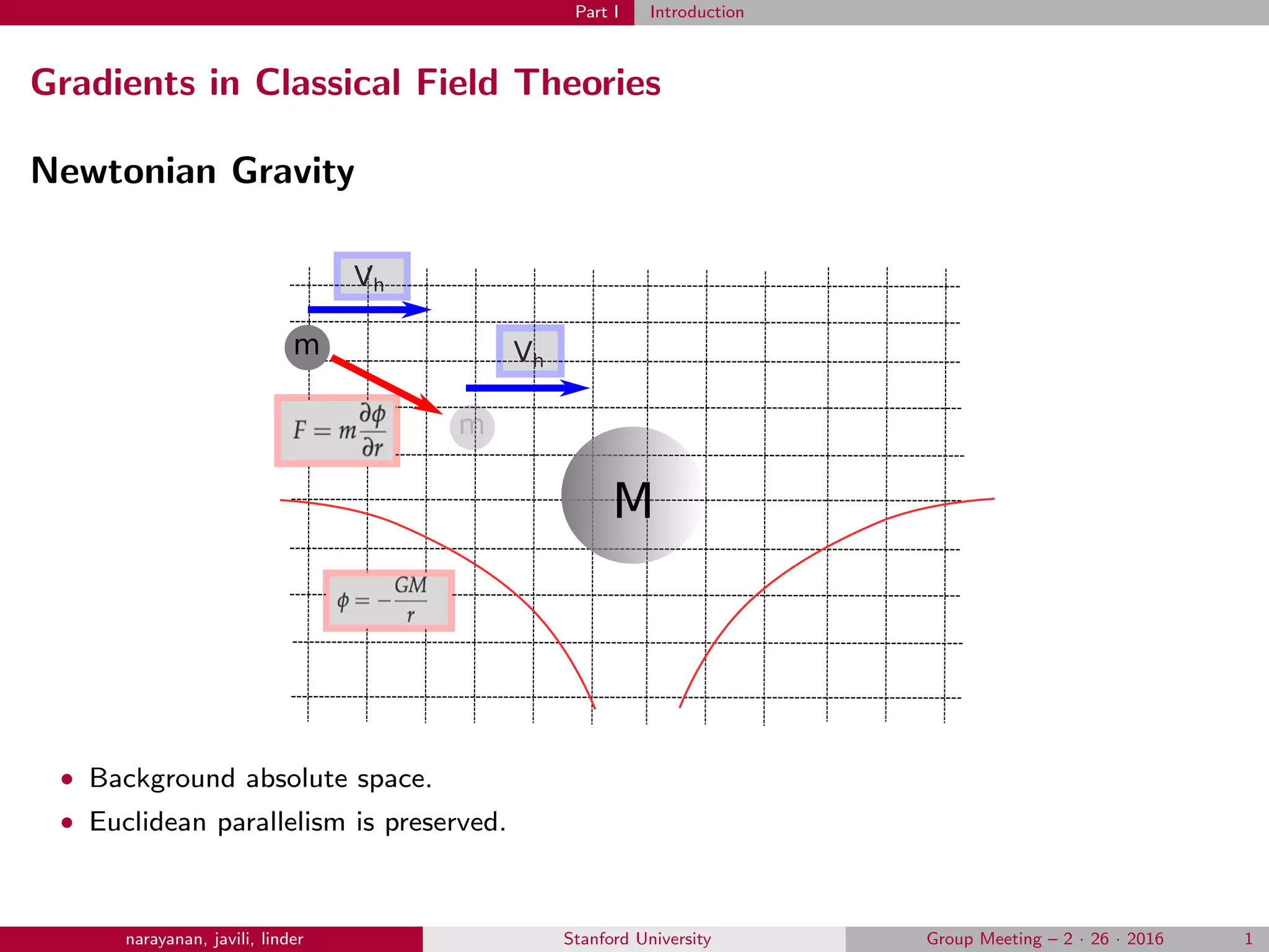
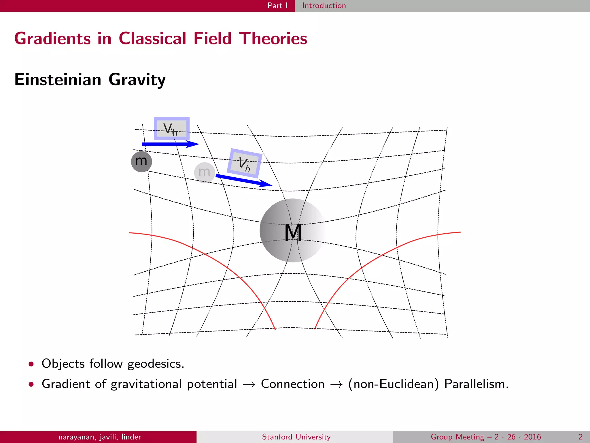
This document introduces higher gradient theories of elasticity. It begins with an overview of how gradients appear in classical field theories like Newtonian gravity and Einsteinian gravity. It then discusses how higher gradients are relevant to continuum mechanics. The remainder of the document outlines the mathematical and variational framework for developing higher gradient elasticity theories. This includes discussions of geometric notions, variational principles, obtaining the strong form of the governing equations, and finite element discretization methods.


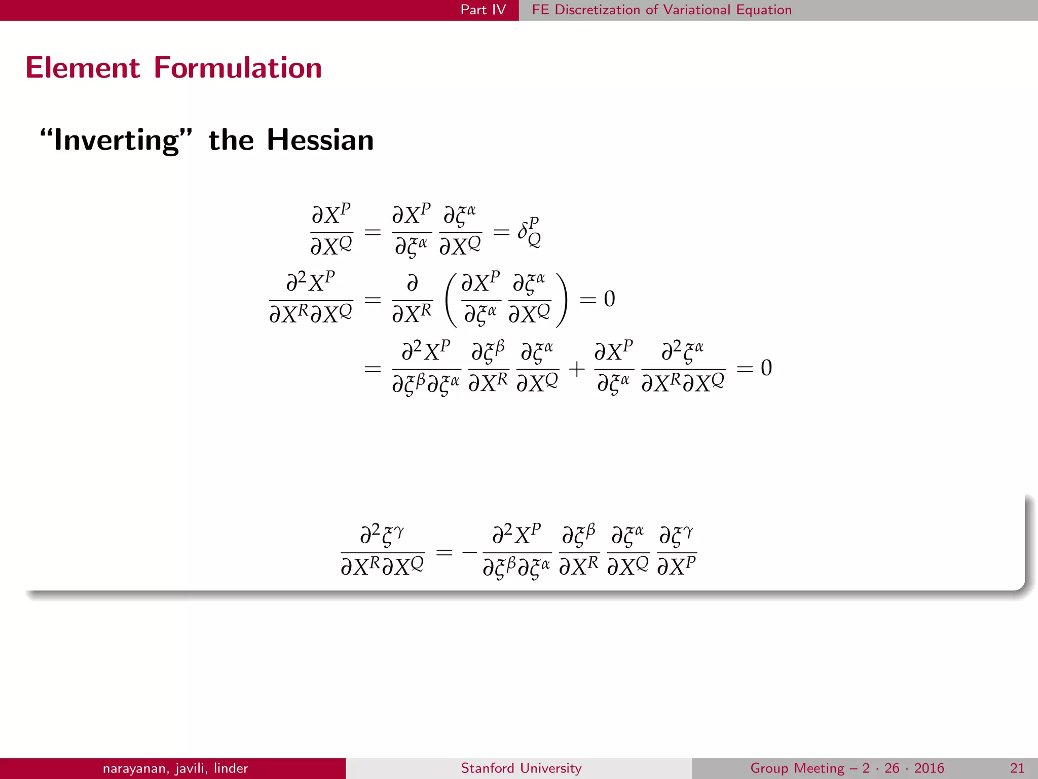
![Part IV FE Discretization of Variational Equation
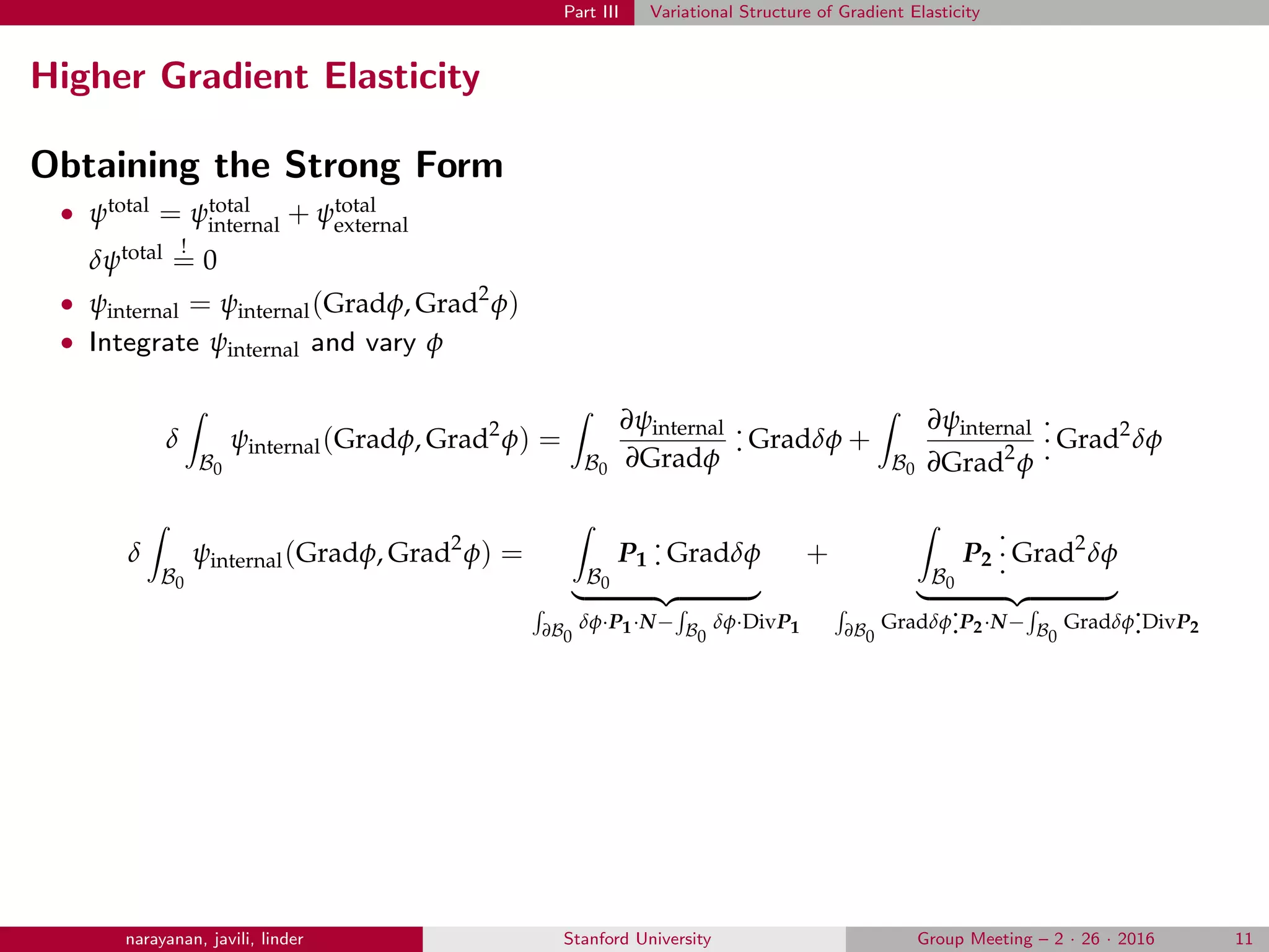
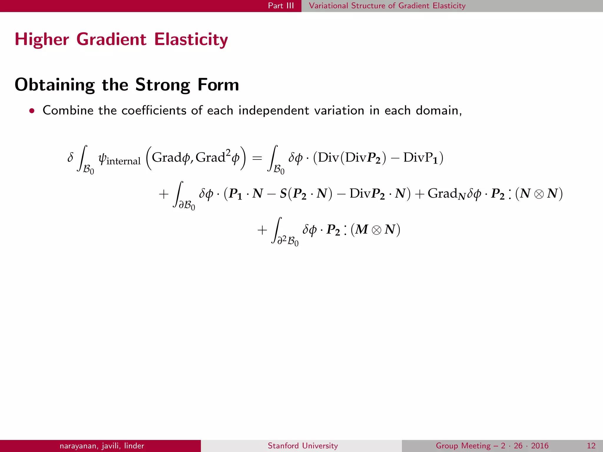
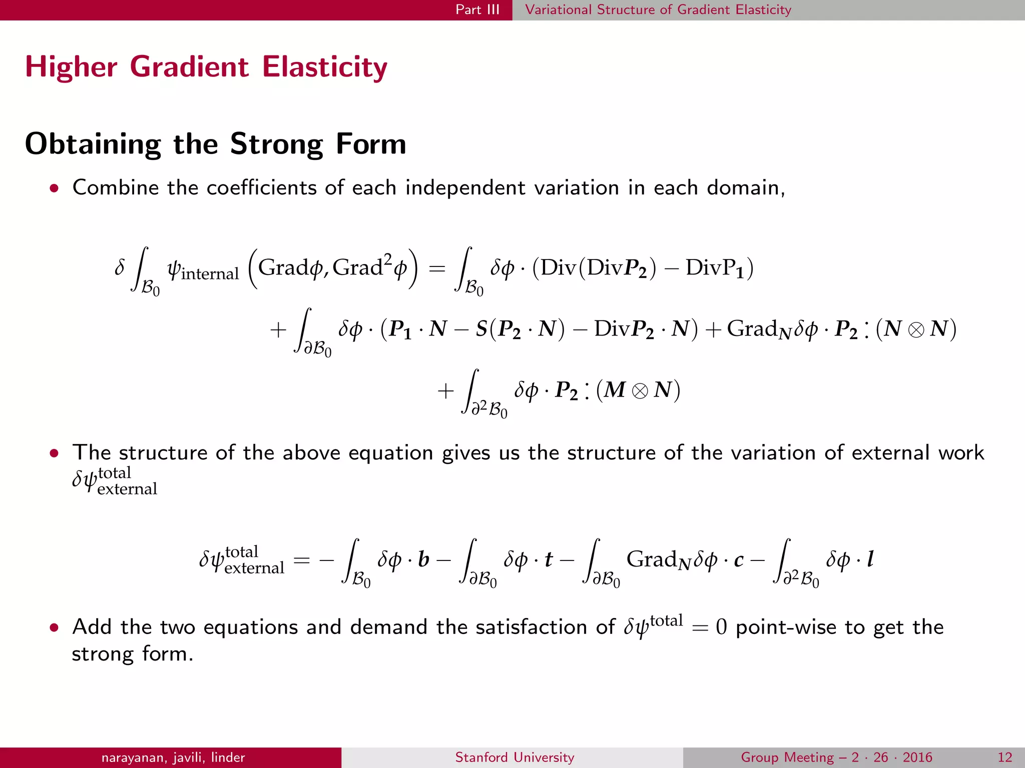
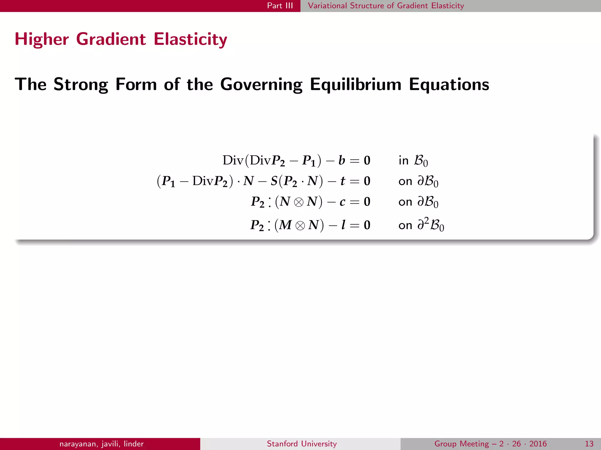
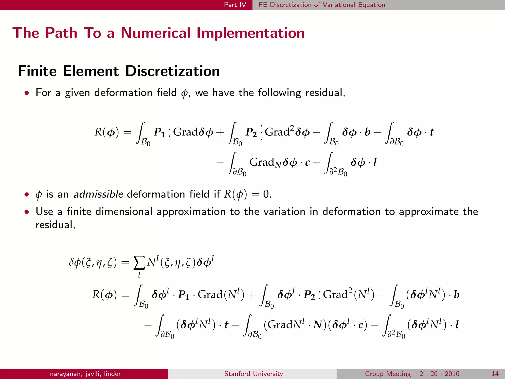
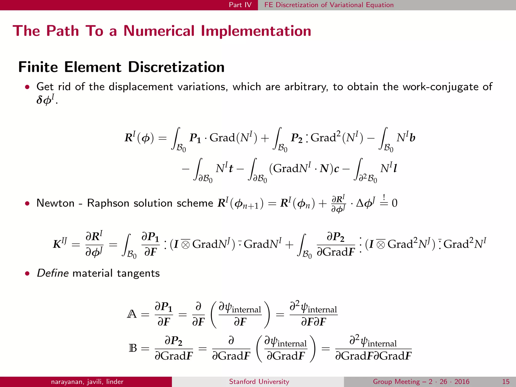
The Path To a Numerical Implementation
Constitutive Equations
• We use the following strain energy density function,
ψinternal =
1
2
µ(F
.
. F − 3 − 2ln(J)) +
1
2
λ
1
2
(J2
− 1) − ln(J) +
1
2
µl2
EAB,CEAB,C
• We have the following component-wise expression for P1 and P2,
[P1]bL = µ([F]bL − [F−T
]bL) +
λ
2
(J2
− 1)[F−T
]bL
+
1
2
µl2
[GradF]bJK([GradF]aJK[F]aL + [F]aJ[GradF]aLK)
[P2]bLM =
µl2
2
[F]bJ([GradF]aLM[F]aJ + [F]aL[GradF]aJM)
narayanan, javili, linder Stanford University Group Meeting – 2 · 26 · 2016 16](https://image.slidesharecdn.com/52078d16-9158-4afe-ab65-aa5fef02ae63-160529161736/75/Introduction-to-second-gradient-theory-of-elasticity-Arjun-Narayanan-24-2048.jpg)
![Part IV FE Discretization of Variational Equation
The Path To a Numerical Implementation
Constitutive Equations
• We have the following component wise expression for A and B
[A]bLgM = µ δb
gδL
M + [F−T
]gL[F−T
]bM + λJ2
[F−T
]gM[F−T
]bL
−
λ
2
(J2
− 1)[F−T
]gL[F−T
]bM +
µl2
2
[GradF]bJK [GradF]gJKδL
M + [GradF]gLKδJ
M
[B]bLMgPQ =
µl2
4
[F]bJ[F]gJ(δL
PδM
Q + δL
QδM
P ) + [F]bP[F]gLδM
Q + [F]bQ[F]gLδM
P
narayanan, javili, linder Stanford University Group Meeting – 2 · 26 · 2016 17](https://image.slidesharecdn.com/52078d16-9158-4afe-ab65-aa5fef02ae63-160529161736/75/Introduction-to-second-gradient-theory-of-elasticity-Arjun-Narayanan-25-2048.jpg)