SlideShare a Scribd company logo
1 
Advanced Finite Element Analysis
Prof. R. KrishnaKumar
Department of Mechanical Engineering
Indian Institute of Technology, Madras
Lecture - 9
In the last class, we were looking at incompressibility.
(Refer Slide Time: 1:01)
Before that, there was a question on what we mean by dot? Say, sigma dot, epsilon dot or
lambda dot, what this dot really means? There is a small confusion. I had said that, said
this before and I am just repeating that; we are not into what is called as rate dependent
phenomena when we talk about plasticity. These rates are pseudo rates. So, sigma dot] is
perfectly equivalent to writing delta sigma, both of them are the same. That is in other
words, delta sigma when divided just by delta t, what is this? Time; time has nothing to
do with your application of load or loading time or whatever it is, it has nothing to do
with that. Just it is a pseudo time to only capture that the loading has to be applied in an
incremental fashion. That is all. So, this lambda dot, sigma dot, epsilon dot in one sense
conveys that the approach is incremental in nature. But we are going to see, there are
2 
some other things that come into picture later in the course, but right now you can say
that sigma dot and delta sigma, they are, both of them are equal.
So, the loading carries itself in time. In one sense the rate of loading is what manifests as
or comes out as sigma dot and so on. But, this rate of loading does not mean that we are
taking into account the inertial effects or rate dependent effects or strain rate effects and
so on. Once you are looking at strain rate effects, then the time should be the correct time.
It cannot be pseudo time. Is that clear? We will, we will give more explanation to it as we
go along in the course, but let us now look at a very important thing called
incompressibility.
Now, what is incompressibility? There was a question again in the last class, when we
finished that what is incompressibility? Incompressibility simply means that there is no
volume change. Incompressibility does not mean that we cannot compress it. We can
compress it, but when you compress it, the compressive strains that are developed are in
such a fashion that there is no change in volume. Is that clear? That is what it means.
(Refer Slide Time: 3:48)
3 
Now, we know that when it is compressible, we will prove it again in a more rigorous
setting later in the course that when incompressibility is the condition then nu equal to
0.5. Now, let us see, look at the difficulties that happens that take place when we have nu
is equal to 0.5. Since this is a material behavior, the culprit is going to be the D matrix.
All of you know that this is the elastic matrix. Now, let us split this D matrix into a part
which is going to be my problem or problematic part and a part which is not going to be
so very problematic part.
(Refer Slide Time: 4:40)
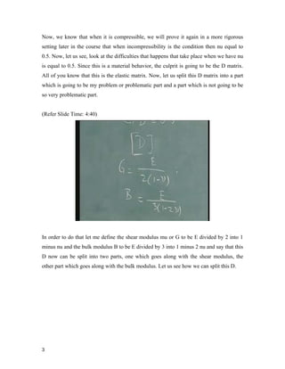
In order to do that let me define the shear modulus mu or G to be E divided by 2 into 1
minus nu and the bulk modulus B to be E divided by 3 into 1 minus 2 nu and say that this
D now can be split into two parts, one which goes along with the shear modulus, the
other part which goes along with the bulk modulus. Let us see how we can split this D.
4 
(Refer Slide Time: 5:25)
This is regular D, we are not talking about dt now; just we are going to look at regular D.
This D can now be written as, say for example, G into 4 by 3 minus 2 by 3 minus 2 by 3
minus 0 0 0, minus 2 by 3 4 by 3 minus 2 by 3 0 0 0 and so on, as one part plus the other
part consists of B into, B is my bulk modulus into and so on. Of course, the last rows are
zeros. Then it is, this becomes 0 0. Yeah, this part, this is zero; this is, no, third is minus 2
by 3 minus 2 by 3 0 0 0; the rest of it, 0 4 by 3 or sorry 1 1 1 and so on. Yeah, this is 6 by
6 matrix; this is a 6 by 6 matrix which of course we are talking about.
5 
(Refer Slide Time: 6:57)
This is the relationship between sigma is equal to D epsilon. So, we are splitting this D
into two parts, what goes into B transpose dB? Now, if you look at these two parts, the
culprit obviously is here, because you have 1 minus 2 nu term here. Now substituting, let
me call this as say DS, first part as DS and second part say as DB to indicate that one part
is formed by shear modulus and the other part formed by bulk modulus, so that my total
K consists of B transpose, instead of D, I am going to say that D shear modulus and bulk
modulus B d omega.
6 
(Refer Slide Time: 7:41)
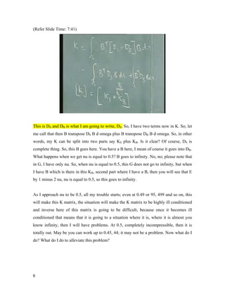
This is DS and DB is what I am going to write, DS. So, I have two terms now in K. So, let
me call that then B transpose DS B d omega plus B transpose DB B d omega. So, in other
words, my K can be split into two parts say KS plus KB. Is it clear? Of course, DS is
complete thing. So, this B goes here. You have a B here, I mean of course it goes into DB.
What happens when we get nu is equal to 0.5? B goes to infinity. No, no; please note that
in G, I have only nu. So, when nu is equal to 0.5, this G does not go to infinity, but when
I have B which is there in this KB, second part where I have a B, then you will see that E
by 1 minus 2 nu, nu is equal to 0.5, so this goes to infinity.
As I approach nu to be 0.5, all my trouble starts; even at 0.49 or 95, 499 and so on, this
will make this K matrix, the situation will make the K matrix to be highly ill conditioned
and inverse here of this matrix is going to be difficult, because once it becomes ill
conditioned that means that it is going to a situation where it is, where it is almost you
know infinity, then I will have problems. At 0.5, completely incompressible, then it is
totally out. May be you can work up to 0.45, 44; it may not be a problem. Now what do I
do? What do I do to alleviate this problem?
7 
In a crude sense, I mean this is not, I am not going to talk total theory; we will come to
that a bit later. In a crude sense you may think that there is a solution. What is the
solution? Solution comes from a possible mistake I may make, use the integration rule.
(Refer Slide Time: 10:58)
Probably you would remember or studied, what is called as rank deficiency or hour
glassing. In our earlier class, we said that there is a particular integration rule I have to
use in order that I can integrate this accurately; polynomial of 2n minus 1 integrated
accurately with an order of n. In other words, we said that for a quadrilateral, I have to
use a 2 by 2 integration. What happens when I reduce this integration, when I go to 1 by
1 rule? I will get into what is called as rank deficiency, what is called as hour glassing.
The rank of the matrix is not sufficient enough for me to invert and make it stable. I will
get into singularity problems and so on. So, there is what is called rank deficiency when I
reduce the numerical integration and so I avoided it. So, I will go for full integration. If it
all I do reduced integration, I do other procedures called stabilization procedures. So, that
is called as hour glassing and in order to avoid hour glassing, I did some what is called as
stabilization procedure or in other words, in other words, you call this as hour glass
control.
8 
In fact, if you had used many of the explicit finite element code, you would see that most
of them use reduced integration and they will have a proper hour glass control. In other
words, by making a small, if I may call it a mistake, mistake within quotes, I got into
some trouble and I got out also by doing some damage exercises. So, major thing is that
that matrix is becoming singular when I did those things. Now, what I am going to do
now is very similar thing; I am going to make the mistake wantonly. How I am going to
do that? Having known that this kind of problems will exist, what I will do is simply take
this and perform an under integration or reduced integration.
In other words, I selectively integrate a part of the K matrix in a reduced fashion. So,
instead of 2 by 2, I may use 1; 1 by 1 row. If I need 3 by 3, I will use 2 by 2 row; I can
reduce the integration, order of integration. So, once I make that decision my problem to
a great extent is solved, because this KB matrix will become now singular. This will not
have, so this, the whole, though I will still have K from here. So, this contribution, this,
this problem of inverting this and going to infinity will not happen. That is called as
selective reduced integration. This problem of inverting this, I will not have difficulty. I
will have difficulty in the sense that that would be automatically taken care of by reduced
integration.
Now, this looks like a crime. People call this as crimes and so on; variational crimes,
common word that is used many times. This looks like a crime, but a beautiful paper by
Semo and Hughes showed that after all what you are doing is very well within the frame
work of variational approach. So, though it looks as if we can do the whole thing by
learning from a mistake, it interestingly has a very good theoretical background as well. It
comes from some of the variational principles which you might not have heard and we
will see that in this course. So, by doing this selective reduced integration, I can in one
word alleviate many of the problems. Is that clear?
How do you find out the order? But, you know the full order of integration that is
required, this depends upon the powers or the the polynomials that are there. That is why
I said 2n minus 1 polynomial is integrated exactly by end point integration rule. So,
9 
depending upon what is that you have, you can find out the exact and then you can reduce
it accordingly. Now, this is fine as far as this kind of simple elastic problem are
concerned and the approach seems to be sort of though not very correct, looks logical.
Now, how do we do a problem like plasticity or some other aspect where I cannot write
this very clearly like DS and DB and so on. Now, various methods have been proposed
and one of the methods which is very popular is called as B-bar method of Hughes. We
will see more theory after we do this. We are going to do the same selective reduced
integration, extend this concept what we have given here. I have not introduced, there is
lot more again simple things that you can talk about this. You will see that this B here
works like a penalty constant, but since we have not done lot more on penalty approach
and all this, I am not commenting on that, but suffice it for me to take me to the next
group of algorithms which come under what are called as B-bar method.
(Refer Slide Time: 18:08)
What essentially B-bar method does is to now alter not this D, but to alter B. After all you
can see that the culprit seems to be in the volumetric part and so can I now split B into
two parts - a deviatoric and a volumetric part and do something to the volumetric part of
K, which results from splitting this B, that B volume. Let us proceed instead of D
10 
splitting B. Yes, what is this B? Correct, the B is the strain displacement relationship; B
is the strain displacement relationship which is epsilon.
(Refer Slide Time: 18:58)
In this case epsilon happens to be B into the degrees of freedom, degrees of freedom,
which you can call this as u hat. Now, there is a difference between u and u hat. Note this
subtle difference between them. u is the displacement of a continuum. Now I am going to
use this because, I need some other, you know, alleviate to define these two separately.
So, u is a displacement of a continuum. In other words, u is a vector which can be written
as say this u is u x comma y and v x comma y. This u hat is the u at the say, nodal
locations; it is at the nodal locations. Suppose I have 1 2 3 4, then u1 u2 v1, u1 u2 u3 u4 v1
v2 v3 v4 that come under u hat. So, B is of course the strain displacement matrix. See, this
is the continuum u. This u and v are the continuum u. This u hat is after this continuum is
discretized and suppose I call this as 1 2 3 and 4, then u hat gives me a vector of the form
say u1 v1 u2 sorry v2 and so on up to u4 v4. This vector is what I call by this u hat.
Yeah, without hat; yes, that is because in the next formulation, I am going to use certain
things with u as well. So, that is why we are looking at this more closely. As you raise
11 
your level of understanding, you have to distinguish between u and u hat or in other
words continuum u and discretized u.
(Refer Slide Time: 21:17)
Say, may be in earlier classes we had put this as B u and understood that this u is this. We
never worried about the continuum u. Sometimes it may be necessary to have that also,
so that strain epsilon we will define it as Su. S is my operator. We will define that again
bit later. So, let us now define it like this. Now of course, B is a matrix. B is a matrix
which consists of say B1 B2 B3 and so on up to B into number of elements.
12 
(Refer Slide Time: 22:14)
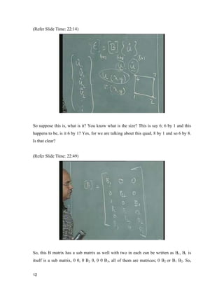
So suppose this is, what is it? You know what is the size? This is say 6; 6 by 1 and this
happens to be, is it 6 by 1? Yes, for we are talking about this quad, 8 by 1 and so 6 by 8.
Is that clear?
(Refer Slide Time: 22:49)
So, this B matrix has a sub matrix as well with two in each can be written as B1, B1 is
itself is a sub matrix, 0 0, 0 B2 0, 0 0 B3, all of them are matrices; 0 B2 or B1 B2. So,
13 
depending upon whether you write epsilon23 or epsilon13 and then B3 0 B1 and B2 B1 B3
B2 or B3, yeah B2 B3. Let us check that out. So, suppose I have epsilon11, this will
become, so that should be B1 0, sorry, it should be B1 B2 yes, just we stick on to the same
thing ….. sorry B2 B1; B2 B1 0 B3 B2 B3 B1. So, let us put it like this. Anyway you know
what this B’s are.
Now, what we are going to do essentially is to split this B into two parts, a dilatational
part and a deviatoric part.
(Refer Slide Time: 24:58)
Let me call this B dilatational part to be say, one-third of, this comes out very easily; B1,
B1 comes from that, this one B1 B2 B3, B1 B2 B3, B1 B2 B3, 0 0 0, 0 0 0, 0 0 0. Now, how
did I get that? One minute, how did I get that? I got this from the fact that the dilatational
part is given by epsilon11 plus epsilon22 plus epsilon33 and similar to what we did for
pressure by 3, so, epsilon 11 22 33 consists of sum of B1 and corresponding to u1, B2
corresponding to u2, B3 corresponding to u3, so, B1 B2 B3, together forms epsilon 11 22
33. So, that is why we had that by 3 and so that gives the dilatational part.
14 
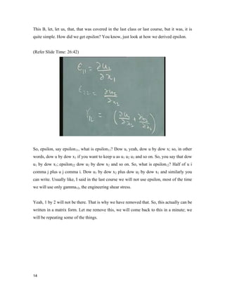
This B, let, let us, that, that was covered in the last class or last course, but it was, it is
quite simple. How did we get epsilon? You know, just look at how we derived epsilon.
(Refer Slide Time: 26:42)
So, epsilon, say epsilon11, what is epsilon11? Dow u, yeah, dow u by dow x; so, in other
words, dow u by dow x1 if you want to keep u as u1 u2 u3 and so on. So, you say that dow
u1 by dow x1; epsilon22 dow u2 by dow x2 and so on. So, what is epsilon12? Half of u i
comma j plus u j comma i. Dow u1 by dow x2 plus dow u2 by dow x1 and similarly you
can write. Usually like, I said in the last course we will not use epsilon, most of the time
we will use only gamma12, the engineering shear stress.
Yeah, 1 by 2 will not be there. That is why we have removed that. So, this actually can be
written in a matrix form. Let me remove this, we will come back to this in a minute; we
will be repeating some of the things.
15 
(Refer Slide Time: 28:13)
This will, can be written in the matrix form as epsilon is equal to u, with first entry being
dow by say dow x1. Suppose, I am only looking at a two dimensional case, you can
extend it very easily to three dimensional case, so that let me see that is epsilon11, next is
epsilon22, say gamma12; only these three I am going to see. Then, this can be written as
dow by dow x1 0 0, 0 dow by dow x2 0. Then I have to multiply, so, first one will be dow
by dow x2 dow by dow x1 0. This would be the, for these three. So, I will have actually,
because 33 was not there, this was all zero. In other words, you can look it at even as just
like that.
16 
(Refer Slide Time: 29:26)
Of course, when I want to have a complete set then, I may, I may have to extend this into
3 rows or rather 3 columns and 6 rows. So, this matrix is what I would call as a S matrix.
Note that this u is my continuum u. This is what now is replaced by N into discretized u.
That is what I called as u hat.
(Refer Slide Time: 30:09)
17 
So S into N into u. Now, let us not worry about the isoparametric; N is our shape
function, obviously so, u hat this is, this is what is called as my u hat and N u. Now, this
multiplied by this S N, this can be written as S N u. So, this S N is what is called as B,
sorry, u hat; that is u hat. So, S N is what is called as B into u hat. So, you can down write
B very easily. Is that clear? Yes; this is for, this for one u. So, if you, if I now put down
all the nodes correspondingly I will have in u, I will have corresponding to all the nodes,
so it will, I will have u1.
(Refer Slide Time: 31:16)
Let me call this as from u1 to u8 to make things clear again. So, u1 u2 u3 u4 u5 u6 u7 and u8.
So, u will be defined in terms of N1 N2 N3 N4. So, how do you write N now? N will be,
now will be 3. See, this will be say, let, let us come back to dimensions of this. Suppose I
am looking at 6; so, 6 here. So, 6 by 1 is equal to, S will be 3, 6 by 3. What will be N? N
will be 3 by 8, sorry and u will be 8 by 1, so that 6, 6 by 3 into 3 by 8 6 by 8 into 8 by 1.
Now, my B matrix I said is 6 by 8. That is what I wrote this as in a form which is, you
know, combining this I wrote it like that, B1 B2. That is why I said B1 is a sub matrix. Is
that clear?
So, symbolically, I mean I am, I am not expanding all this.
18 
(Refer Slide Time: 33:12)
Symbolically I am writing it so that you will, I mean you know here after I will not write
u1 u2, I will just say that this is the u vector. That is all. Fine; so please note that the
number of degrees of freedom also entered into this B matrix.
(Refer Slide Time: 33:39)
So, this B matrix is the one which I say can be split up into two parts. One is B
dilatational part plus B deviatoric part; B dilatational part and B deviatoric part. The
19 
dilatational part consists of one-third of B’s, one-third of say, the first part of B is or in
other words, the dilatational part comes from the fact that it is epsilon 11 plus 22 plus 33.
So, I can write this say, as B1 B2 B3; it is the same B1 B2 B3, B1 B2 B3. This is for, actually
what we did here note that this is for 2D case. If I have to actually, this a small, I think we
did not do this correctly; sorry, one minute.
(Refer Slide Time: 35:00)
We did not do that correctly, because we are looking at 3D case. So 3D case is, actually
we have extended it to 3D case. So, in 3D case this is equal to 6 by 1 and S is, there are
how many rows? 3; so how many, how many columns? 3 columns and 6 rows, so, 6 into
3. Then here it is 3 into, say for example, you are looking at a brick element now. Brick
element, 8; 8 into, yes, 8 into 2, number of degrees of freedom, 16. So this should be 3
into 16; so, 16 into 1. Which one? Yeah, 8 into 3, 24 right, not 62, not 2; 3, so, 3 into 24
and 24 into 1, 24 into 1; correct. So, 6 into 3, 3 into 24, 24 into 1, so that now B matrix is
actually S into N, which means 6 into 24; 6 into 24 and so each of this B1 are …….
20 
(Refer Slide Time: 36:31)
Yeah, so, that is why now B dilatational one-third is written as B1 B2 B3. These are
matrices, now you know what they are? B1 B2 B3, B1 B2 B3, 0 0 0, 0 0 0, 0 0 0 ; one-third.
Yes; wait a minute. Let me finish it. So, plus I have a deviatoric part such that the sum of
this deviatoric plus dilatational part will give me B. Is that clear?
No; I am splitting this B into a dilatational part in the same fashion that I can split strains,
because after all these are strain displacement relationship. So, in the same fashion I can
split strains I am splitting B into the dilatational part and deviatoric part. So, the
dilatational part is this and deviatoric part is the other one. So, in fact if I am going to
write down these two before we write down the equation and substitute this into my K
matrix, you will see that I can write that down as my K matrix or KT matrix, can be
written as integral omega say B deviatoric plus B dilatational.
21 
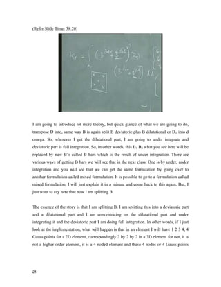
(Refer Slide Time: 38:20)
I am going to introduce lot more theory, but quick glance of what we are going to do,
transpose D into, same way B is again split B deviatoric plus B dilatational or DT into d
omega. So, wherever I get the dilatational part, I am going to under integrate and
deviatoric part is full integration. So, in other words, this B1 B2 what you see here will be
replaced by new B’s called B bars which is the result of under integration. There are
various ways of getting B bars we will see that in the next class. One is by under, under
integration and you will see that we can get the same formulation by going over to
another formulation called mixed formulation. It is possible to go to a formulation called
mixed formulation; I will just explain it in a minute and come back to this again. But, I
just want to say here that now I am splitting B.
The essence of the story is that I am splitting B. I am splitting this into a deviatoric part
and a dilatational part and I am concentrating on the dilatational part and under
integrating it and the deviatoric part I am doing full integration. In other words, if I just
look at the implementation, what will happen is that in an element I will have 1 2 3 4, 4
Gauss points for a 2D element, correspondingly 2 by 2 by 2 in a 3D element for not, it is
not a higher order element, it is a 4 noded element and these 4 nodes or 4 Gauss points
22 
rather are used to integrate the deviatoric part and I will use one Gauss point at the center
to integrate the dilatational part. So, this is called as selective reduced integration.
Yes. Yeah, usually you do not consider them, but you take that separately as deviatoric
DT. That is why we would call that as a B-bar. You will see how it comes up in the next
part of the derivation in the mixed formulation, but you will, usually you take deviatoric
part separately into DT, dilatational part separately. So, you will have deviatoric DT
deviatoric, dilatational DT dilatational. These are the two things that you will take them
up separately. In other words, it is not very correct to split that. In fact, I should have
written this as B consisting of, actually this comes from my P matrix, from the B
transpose sigma.
(Refer Slide Time: 41:51)
Actually I should have, I should not have written it like this. Actually we should have
written it as B transpose sigma d omega and from here I should have written this as B
deviatoric plus B dilatational sigma d omega and so on. In other words, you will have
only two parts B deviatoric d B deviatoric plus dilatational part. So, that is what you
under integrate. So, you will have, actually if you really look at it, you will have 5 Gauss
points.
23 
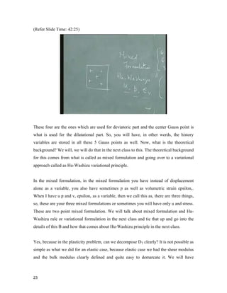
(Refer Slide Time: 42:25)
These four are the ones which are used for deviatoric part and the center Gauss point is
what is used for the dilatational part. So, you will have, in other words, the history
variables are stored in all these 5 Gauss points as well. Now, what is the theoretical
background? We will, we will do that in the next class to this. The theoretical background
for this comes from what is called as mixed formulation and going over to a variational
approach called as Hu-Washizu variational principle.
In the mixed formulation, in the mixed formulation you have instead of displacement
alone as a variable, you also have sometimes p as well as volumetric strain epsilonv.
When I have u p and v, epsilonv as a variable, then we call this as, there are three things,
so, these are your three mixed formulations or sometimes you will have only u and stress.
These are two point mixed formulation. We will talk about mixed formulation and Hu-
Washizu rule or variational formulation in the next class and tie that up and go into the
details of this B and how that comes about Hu-Washizu principle in the next class.
Yes, because in the plasticity problem, can we decompose DT clearly? It is not possible as
simple as what we did for an elastic case, because elastic case we had the shear modulus
and the bulk modulus clearly defined and quite easy to demarcate it. We will have
24 
problems when we do that in the plastic, in the plasticity part of it. So, let us look at the
mixed formulation and then talk about the rest of it.

More Related Content

Viewers also liked

DUZA- LINEA WORKSAFE
DUZA- LINEA WORKSAFEDUZA- LINEA WORKSAFE
DUZA- LINEA WORKSAFE
DUZA IMPORTACIONES
 
ALTENBURG 204- PROMOS
ALTENBURG 204- PROMOSALTENBURG 204- PROMOS
ALTENBURG 204- PROMOS
DUZA IMPORTACIONES
 
DUZA- LINEA VIDRIOS CIV -CISPER
DUZA- LINEA VIDRIOS CIV -CISPERDUZA- LINEA VIDRIOS CIV -CISPER
DUZA- LINEA VIDRIOS CIV -CISPER
DUZA IMPORTACIONES
 
DUZA- LINEA BANDEIRANTES
DUZA- LINEA BANDEIRANTESDUZA- LINEA BANDEIRANTES
DUZA- LINEA BANDEIRANTES
DUZA IMPORTACIONES
 
LINEA ASADOR FAT
LINEA ASADOR FATLINEA ASADOR FAT
LINEA ASADOR FAT
DUZA IMPORTACIONES
 
DUZA- LINEA MUNDIAL TIJERAS
DUZA- LINEA MUNDIAL TIJERASDUZA- LINEA MUNDIAL TIJERAS
DUZA- LINEA MUNDIAL TIJERAS
DUZA IMPORTACIONES
 
DUZA LINEA INOX
DUZA LINEA INOXDUZA LINEA INOX
DUZA LINEA INOX
DUZA IMPORTACIONES
 
PROMOS- CONSERVADORAS Y CAMPING
PROMOS- CONSERVADORAS Y CAMPINGPROMOS- CONSERVADORAS Y CAMPING
PROMOS- CONSERVADORAS Y CAMPING
DUZA IMPORTACIONES
 
DUZA- LINEA ALUMINIO PATO BRANCO
DUZA- LINEA ALUMINIO PATO BRANCODUZA- LINEA ALUMINIO PATO BRANCO
DUZA- LINEA ALUMINIO PATO BRANCO
DUZA IMPORTACIONES
 
DUZA- LINEA DESESPLAST
DUZA- LINEA DESESPLASTDUZA- LINEA DESESPLAST
DUZA- LINEA DESESPLAST
DUZA IMPORTACIONES
 
DUZA- LINEA ALTENBURG DE ALMOHADAS
DUZA- LINEA ALTENBURG DE ALMOHADASDUZA- LINEA ALTENBURG DE ALMOHADAS
DUZA- LINEA ALTENBURG DE ALMOHADAS
DUZA IMPORTACIONES
 

Viewers also liked (14)

Lec6
Lec6Lec6
Lec6
 
DUZA- LINEA WORKSAFE
DUZA- LINEA WORKSAFEDUZA- LINEA WORKSAFE
DUZA- LINEA WORKSAFE
 
Lec12
Lec12Lec12
Lec12
 
ALTENBURG 204- PROMOS
ALTENBURG 204- PROMOSALTENBURG 204- PROMOS
ALTENBURG 204- PROMOS
 
DUZA- LINEA VIDRIOS CIV -CISPER
DUZA- LINEA VIDRIOS CIV -CISPERDUZA- LINEA VIDRIOS CIV -CISPER
DUZA- LINEA VIDRIOS CIV -CISPER
 
Lec2
Lec2Lec2
Lec2
 
DUZA- LINEA BANDEIRANTES
DUZA- LINEA BANDEIRANTESDUZA- LINEA BANDEIRANTES
DUZA- LINEA BANDEIRANTES
 
LINEA ASADOR FAT
LINEA ASADOR FATLINEA ASADOR FAT
LINEA ASADOR FAT
 
DUZA- LINEA MUNDIAL TIJERAS
DUZA- LINEA MUNDIAL TIJERASDUZA- LINEA MUNDIAL TIJERAS
DUZA- LINEA MUNDIAL TIJERAS
 
DUZA LINEA INOX
DUZA LINEA INOXDUZA LINEA INOX
DUZA LINEA INOX
 
PROMOS- CONSERVADORAS Y CAMPING
PROMOS- CONSERVADORAS Y CAMPINGPROMOS- CONSERVADORAS Y CAMPING
PROMOS- CONSERVADORAS Y CAMPING
 
DUZA- LINEA ALUMINIO PATO BRANCO
DUZA- LINEA ALUMINIO PATO BRANCODUZA- LINEA ALUMINIO PATO BRANCO
DUZA- LINEA ALUMINIO PATO BRANCO
 
DUZA- LINEA DESESPLAST
DUZA- LINEA DESESPLASTDUZA- LINEA DESESPLAST
DUZA- LINEA DESESPLAST
 
DUZA- LINEA ALTENBURG DE ALMOHADAS
DUZA- LINEA ALTENBURG DE ALMOHADASDUZA- LINEA ALTENBURG DE ALMOHADAS
DUZA- LINEA ALTENBURG DE ALMOHADAS
 

Similar to Lec9

AP Calculus - Mini Exam Review
AP Calculus - Mini Exam ReviewAP Calculus - Mini Exam Review
AP Calculus - Mini Exam Reviewk_ina
 
Lec58
Lec58Lec58
lec21.pdf
lec21.pdflec21.pdf
lec21.pdf
RISHABHJAIN27097
 
Element distinctness lower bounds
Element distinctness lower boundsElement distinctness lower bounds
Element distinctness lower bounds
Rajendran
 
Programming methodology lecture06
Programming methodology lecture06Programming methodology lecture06
Programming methodology lecture06NYversity
 
Lec10
Lec10Lec10
Lec49
Lec49Lec49
Algebra prelims
Algebra prelimsAlgebra prelims
Algebra prelims
TrabahoLang
 
Lec28
Lec28Lec28
Lec60
Lec60Lec60
Lec40
Lec40Lec40
Lec57
Lec57Lec57
Lec39
Lec39Lec39
Programming methodology lecture07
Programming methodology lecture07Programming methodology lecture07
Programming methodology lecture07NYversity
 

Similar to Lec9 (20)

Lec12
Lec12Lec12
Lec12
 
Calc ii seriesconvergence
Calc ii seriesconvergenceCalc ii seriesconvergence
Calc ii seriesconvergence
 
AP Calculus - Mini Exam Review
AP Calculus - Mini Exam ReviewAP Calculus - Mini Exam Review
AP Calculus - Mini Exam Review
 
Lec58
Lec58Lec58
Lec58
 
lec21.pdf
lec21.pdflec21.pdf
lec21.pdf
 
Element distinctness lower bounds
Element distinctness lower boundsElement distinctness lower bounds
Element distinctness lower bounds
 
Programming methodology lecture06
Programming methodology lecture06Programming methodology lecture06
Programming methodology lecture06
 
Lec10
Lec10Lec10
Lec10
 
Lec49
Lec49Lec49
Lec49
 
Calc ii complete
Calc ii completeCalc ii complete
Calc ii complete
 
Algebra prelims
Algebra prelimsAlgebra prelims
Algebra prelims
 
Lec1
Lec1Lec1
Lec1
 
Lec28
Lec28Lec28
Lec28
 
Lec60
Lec60Lec60
Lec60
 
Lec7
Lec7Lec7
Lec7
 
Lec40
Lec40Lec40
Lec40
 
Lec57
Lec57Lec57
Lec57
 
Lec39
Lec39Lec39
Lec39
 
Wtpc(1)
Wtpc(1)Wtpc(1)
Wtpc(1)
 
Programming methodology lecture07
Programming methodology lecture07Programming methodology lecture07
Programming methodology lecture07
 

Lec9

  • 1. 1  Advanced Finite Element Analysis Prof. R. KrishnaKumar Department of Mechanical Engineering Indian Institute of Technology, Madras Lecture - 9 In the last class, we were looking at incompressibility. (Refer Slide Time: 1:01) Before that, there was a question on what we mean by dot? Say, sigma dot, epsilon dot or lambda dot, what this dot really means? There is a small confusion. I had said that, said this before and I am just repeating that; we are not into what is called as rate dependent phenomena when we talk about plasticity. These rates are pseudo rates. So, sigma dot] is perfectly equivalent to writing delta sigma, both of them are the same. That is in other words, delta sigma when divided just by delta t, what is this? Time; time has nothing to do with your application of load or loading time or whatever it is, it has nothing to do with that. Just it is a pseudo time to only capture that the loading has to be applied in an incremental fashion. That is all. So, this lambda dot, sigma dot, epsilon dot in one sense conveys that the approach is incremental in nature. But we are going to see, there are
  • 2. 2  some other things that come into picture later in the course, but right now you can say that sigma dot and delta sigma, they are, both of them are equal. So, the loading carries itself in time. In one sense the rate of loading is what manifests as or comes out as sigma dot and so on. But, this rate of loading does not mean that we are taking into account the inertial effects or rate dependent effects or strain rate effects and so on. Once you are looking at strain rate effects, then the time should be the correct time. It cannot be pseudo time. Is that clear? We will, we will give more explanation to it as we go along in the course, but let us now look at a very important thing called incompressibility. Now, what is incompressibility? There was a question again in the last class, when we finished that what is incompressibility? Incompressibility simply means that there is no volume change. Incompressibility does not mean that we cannot compress it. We can compress it, but when you compress it, the compressive strains that are developed are in such a fashion that there is no change in volume. Is that clear? That is what it means. (Refer Slide Time: 3:48)
  • 3. 3  Now, we know that when it is compressible, we will prove it again in a more rigorous setting later in the course that when incompressibility is the condition then nu equal to 0.5. Now, let us see, look at the difficulties that happens that take place when we have nu is equal to 0.5. Since this is a material behavior, the culprit is going to be the D matrix. All of you know that this is the elastic matrix. Now, let us split this D matrix into a part which is going to be my problem or problematic part and a part which is not going to be so very problematic part. (Refer Slide Time: 4:40) In order to do that let me define the shear modulus mu or G to be E divided by 2 into 1 minus nu and the bulk modulus B to be E divided by 3 into 1 minus 2 nu and say that this D now can be split into two parts, one which goes along with the shear modulus, the other part which goes along with the bulk modulus. Let us see how we can split this D.
  • 4. 4  (Refer Slide Time: 5:25) This is regular D, we are not talking about dt now; just we are going to look at regular D. This D can now be written as, say for example, G into 4 by 3 minus 2 by 3 minus 2 by 3 minus 0 0 0, minus 2 by 3 4 by 3 minus 2 by 3 0 0 0 and so on, as one part plus the other part consists of B into, B is my bulk modulus into and so on. Of course, the last rows are zeros. Then it is, this becomes 0 0. Yeah, this part, this is zero; this is, no, third is minus 2 by 3 minus 2 by 3 0 0 0; the rest of it, 0 4 by 3 or sorry 1 1 1 and so on. Yeah, this is 6 by 6 matrix; this is a 6 by 6 matrix which of course we are talking about.
  • 5. 5  (Refer Slide Time: 6:57) This is the relationship between sigma is equal to D epsilon. So, we are splitting this D into two parts, what goes into B transpose dB? Now, if you look at these two parts, the culprit obviously is here, because you have 1 minus 2 nu term here. Now substituting, let me call this as say DS, first part as DS and second part say as DB to indicate that one part is formed by shear modulus and the other part formed by bulk modulus, so that my total K consists of B transpose, instead of D, I am going to say that D shear modulus and bulk modulus B d omega.
  • 6. 6  (Refer Slide Time: 7:41) This is DS and DB is what I am going to write, DS. So, I have two terms now in K. So, let me call that then B transpose DS B d omega plus B transpose DB B d omega. So, in other words, my K can be split into two parts say KS plus KB. Is it clear? Of course, DS is complete thing. So, this B goes here. You have a B here, I mean of course it goes into DB. What happens when we get nu is equal to 0.5? B goes to infinity. No, no; please note that in G, I have only nu. So, when nu is equal to 0.5, this G does not go to infinity, but when I have B which is there in this KB, second part where I have a B, then you will see that E by 1 minus 2 nu, nu is equal to 0.5, so this goes to infinity. As I approach nu to be 0.5, all my trouble starts; even at 0.49 or 95, 499 and so on, this will make this K matrix, the situation will make the K matrix to be highly ill conditioned and inverse here of this matrix is going to be difficult, because once it becomes ill conditioned that means that it is going to a situation where it is, where it is almost you know infinity, then I will have problems. At 0.5, completely incompressible, then it is totally out. May be you can work up to 0.45, 44; it may not be a problem. Now what do I do? What do I do to alleviate this problem?
  • 7. 7  In a crude sense, I mean this is not, I am not going to talk total theory; we will come to that a bit later. In a crude sense you may think that there is a solution. What is the solution? Solution comes from a possible mistake I may make, use the integration rule. (Refer Slide Time: 10:58) Probably you would remember or studied, what is called as rank deficiency or hour glassing. In our earlier class, we said that there is a particular integration rule I have to use in order that I can integrate this accurately; polynomial of 2n minus 1 integrated accurately with an order of n. In other words, we said that for a quadrilateral, I have to use a 2 by 2 integration. What happens when I reduce this integration, when I go to 1 by 1 rule? I will get into what is called as rank deficiency, what is called as hour glassing. The rank of the matrix is not sufficient enough for me to invert and make it stable. I will get into singularity problems and so on. So, there is what is called rank deficiency when I reduce the numerical integration and so I avoided it. So, I will go for full integration. If it all I do reduced integration, I do other procedures called stabilization procedures. So, that is called as hour glassing and in order to avoid hour glassing, I did some what is called as stabilization procedure or in other words, in other words, you call this as hour glass control.
  • 8. 8  In fact, if you had used many of the explicit finite element code, you would see that most of them use reduced integration and they will have a proper hour glass control. In other words, by making a small, if I may call it a mistake, mistake within quotes, I got into some trouble and I got out also by doing some damage exercises. So, major thing is that that matrix is becoming singular when I did those things. Now, what I am going to do now is very similar thing; I am going to make the mistake wantonly. How I am going to do that? Having known that this kind of problems will exist, what I will do is simply take this and perform an under integration or reduced integration. In other words, I selectively integrate a part of the K matrix in a reduced fashion. So, instead of 2 by 2, I may use 1; 1 by 1 row. If I need 3 by 3, I will use 2 by 2 row; I can reduce the integration, order of integration. So, once I make that decision my problem to a great extent is solved, because this KB matrix will become now singular. This will not have, so this, the whole, though I will still have K from here. So, this contribution, this, this problem of inverting this and going to infinity will not happen. That is called as selective reduced integration. This problem of inverting this, I will not have difficulty. I will have difficulty in the sense that that would be automatically taken care of by reduced integration. Now, this looks like a crime. People call this as crimes and so on; variational crimes, common word that is used many times. This looks like a crime, but a beautiful paper by Semo and Hughes showed that after all what you are doing is very well within the frame work of variational approach. So, though it looks as if we can do the whole thing by learning from a mistake, it interestingly has a very good theoretical background as well. It comes from some of the variational principles which you might not have heard and we will see that in this course. So, by doing this selective reduced integration, I can in one word alleviate many of the problems. Is that clear? How do you find out the order? But, you know the full order of integration that is required, this depends upon the powers or the the polynomials that are there. That is why I said 2n minus 1 polynomial is integrated exactly by end point integration rule. So,
  • 9. 9  depending upon what is that you have, you can find out the exact and then you can reduce it accordingly. Now, this is fine as far as this kind of simple elastic problem are concerned and the approach seems to be sort of though not very correct, looks logical. Now, how do we do a problem like plasticity or some other aspect where I cannot write this very clearly like DS and DB and so on. Now, various methods have been proposed and one of the methods which is very popular is called as B-bar method of Hughes. We will see more theory after we do this. We are going to do the same selective reduced integration, extend this concept what we have given here. I have not introduced, there is lot more again simple things that you can talk about this. You will see that this B here works like a penalty constant, but since we have not done lot more on penalty approach and all this, I am not commenting on that, but suffice it for me to take me to the next group of algorithms which come under what are called as B-bar method. (Refer Slide Time: 18:08) What essentially B-bar method does is to now alter not this D, but to alter B. After all you can see that the culprit seems to be in the volumetric part and so can I now split B into two parts - a deviatoric and a volumetric part and do something to the volumetric part of K, which results from splitting this B, that B volume. Let us proceed instead of D
  • 10. 10  splitting B. Yes, what is this B? Correct, the B is the strain displacement relationship; B is the strain displacement relationship which is epsilon. (Refer Slide Time: 18:58) In this case epsilon happens to be B into the degrees of freedom, degrees of freedom, which you can call this as u hat. Now, there is a difference between u and u hat. Note this subtle difference between them. u is the displacement of a continuum. Now I am going to use this because, I need some other, you know, alleviate to define these two separately. So, u is a displacement of a continuum. In other words, u is a vector which can be written as say this u is u x comma y and v x comma y. This u hat is the u at the say, nodal locations; it is at the nodal locations. Suppose I have 1 2 3 4, then u1 u2 v1, u1 u2 u3 u4 v1 v2 v3 v4 that come under u hat. So, B is of course the strain displacement matrix. See, this is the continuum u. This u and v are the continuum u. This u hat is after this continuum is discretized and suppose I call this as 1 2 3 and 4, then u hat gives me a vector of the form say u1 v1 u2 sorry v2 and so on up to u4 v4. This vector is what I call by this u hat. Yeah, without hat; yes, that is because in the next formulation, I am going to use certain things with u as well. So, that is why we are looking at this more closely. As you raise
  • 11. 11  your level of understanding, you have to distinguish between u and u hat or in other words continuum u and discretized u. (Refer Slide Time: 21:17) Say, may be in earlier classes we had put this as B u and understood that this u is this. We never worried about the continuum u. Sometimes it may be necessary to have that also, so that strain epsilon we will define it as Su. S is my operator. We will define that again bit later. So, let us now define it like this. Now of course, B is a matrix. B is a matrix which consists of say B1 B2 B3 and so on up to B into number of elements.
  • 12. 12  (Refer Slide Time: 22:14) So suppose this is, what is it? You know what is the size? This is say 6; 6 by 1 and this happens to be, is it 6 by 1? Yes, for we are talking about this quad, 8 by 1 and so 6 by 8. Is that clear? (Refer Slide Time: 22:49) So, this B matrix has a sub matrix as well with two in each can be written as B1, B1 is itself is a sub matrix, 0 0, 0 B2 0, 0 0 B3, all of them are matrices; 0 B2 or B1 B2. So,
  • 13. 13  depending upon whether you write epsilon23 or epsilon13 and then B3 0 B1 and B2 B1 B3 B2 or B3, yeah B2 B3. Let us check that out. So, suppose I have epsilon11, this will become, so that should be B1 0, sorry, it should be B1 B2 yes, just we stick on to the same thing ….. sorry B2 B1; B2 B1 0 B3 B2 B3 B1. So, let us put it like this. Anyway you know what this B’s are. Now, what we are going to do essentially is to split this B into two parts, a dilatational part and a deviatoric part. (Refer Slide Time: 24:58) Let me call this B dilatational part to be say, one-third of, this comes out very easily; B1, B1 comes from that, this one B1 B2 B3, B1 B2 B3, B1 B2 B3, 0 0 0, 0 0 0, 0 0 0. Now, how did I get that? One minute, how did I get that? I got this from the fact that the dilatational part is given by epsilon11 plus epsilon22 plus epsilon33 and similar to what we did for pressure by 3, so, epsilon 11 22 33 consists of sum of B1 and corresponding to u1, B2 corresponding to u2, B3 corresponding to u3, so, B1 B2 B3, together forms epsilon 11 22 33. So, that is why we had that by 3 and so that gives the dilatational part.
  • 14. 14  This B, let, let us, that, that was covered in the last class or last course, but it was, it is quite simple. How did we get epsilon? You know, just look at how we derived epsilon. (Refer Slide Time: 26:42) So, epsilon, say epsilon11, what is epsilon11? Dow u, yeah, dow u by dow x; so, in other words, dow u by dow x1 if you want to keep u as u1 u2 u3 and so on. So, you say that dow u1 by dow x1; epsilon22 dow u2 by dow x2 and so on. So, what is epsilon12? Half of u i comma j plus u j comma i. Dow u1 by dow x2 plus dow u2 by dow x1 and similarly you can write. Usually like, I said in the last course we will not use epsilon, most of the time we will use only gamma12, the engineering shear stress. Yeah, 1 by 2 will not be there. That is why we have removed that. So, this actually can be written in a matrix form. Let me remove this, we will come back to this in a minute; we will be repeating some of the things.
  • 15. 15  (Refer Slide Time: 28:13) This will, can be written in the matrix form as epsilon is equal to u, with first entry being dow by say dow x1. Suppose, I am only looking at a two dimensional case, you can extend it very easily to three dimensional case, so that let me see that is epsilon11, next is epsilon22, say gamma12; only these three I am going to see. Then, this can be written as dow by dow x1 0 0, 0 dow by dow x2 0. Then I have to multiply, so, first one will be dow by dow x2 dow by dow x1 0. This would be the, for these three. So, I will have actually, because 33 was not there, this was all zero. In other words, you can look it at even as just like that.
  • 16. 16  (Refer Slide Time: 29:26) Of course, when I want to have a complete set then, I may, I may have to extend this into 3 rows or rather 3 columns and 6 rows. So, this matrix is what I would call as a S matrix. Note that this u is my continuum u. This is what now is replaced by N into discretized u. That is what I called as u hat. (Refer Slide Time: 30:09)
  • 17. 17  So S into N into u. Now, let us not worry about the isoparametric; N is our shape function, obviously so, u hat this is, this is what is called as my u hat and N u. Now, this multiplied by this S N, this can be written as S N u. So, this S N is what is called as B, sorry, u hat; that is u hat. So, S N is what is called as B into u hat. So, you can down write B very easily. Is that clear? Yes; this is for, this for one u. So, if you, if I now put down all the nodes correspondingly I will have in u, I will have corresponding to all the nodes, so it will, I will have u1. (Refer Slide Time: 31:16) Let me call this as from u1 to u8 to make things clear again. So, u1 u2 u3 u4 u5 u6 u7 and u8. So, u will be defined in terms of N1 N2 N3 N4. So, how do you write N now? N will be, now will be 3. See, this will be say, let, let us come back to dimensions of this. Suppose I am looking at 6; so, 6 here. So, 6 by 1 is equal to, S will be 3, 6 by 3. What will be N? N will be 3 by 8, sorry and u will be 8 by 1, so that 6, 6 by 3 into 3 by 8 6 by 8 into 8 by 1. Now, my B matrix I said is 6 by 8. That is what I wrote this as in a form which is, you know, combining this I wrote it like that, B1 B2. That is why I said B1 is a sub matrix. Is that clear? So, symbolically, I mean I am, I am not expanding all this.
  • 18. 18  (Refer Slide Time: 33:12) Symbolically I am writing it so that you will, I mean you know here after I will not write u1 u2, I will just say that this is the u vector. That is all. Fine; so please note that the number of degrees of freedom also entered into this B matrix. (Refer Slide Time: 33:39) So, this B matrix is the one which I say can be split up into two parts. One is B dilatational part plus B deviatoric part; B dilatational part and B deviatoric part. The
  • 19. 19  dilatational part consists of one-third of B’s, one-third of say, the first part of B is or in other words, the dilatational part comes from the fact that it is epsilon 11 plus 22 plus 33. So, I can write this say, as B1 B2 B3; it is the same B1 B2 B3, B1 B2 B3. This is for, actually what we did here note that this is for 2D case. If I have to actually, this a small, I think we did not do this correctly; sorry, one minute. (Refer Slide Time: 35:00) We did not do that correctly, because we are looking at 3D case. So 3D case is, actually we have extended it to 3D case. So, in 3D case this is equal to 6 by 1 and S is, there are how many rows? 3; so how many, how many columns? 3 columns and 6 rows, so, 6 into 3. Then here it is 3 into, say for example, you are looking at a brick element now. Brick element, 8; 8 into, yes, 8 into 2, number of degrees of freedom, 16. So this should be 3 into 16; so, 16 into 1. Which one? Yeah, 8 into 3, 24 right, not 62, not 2; 3, so, 3 into 24 and 24 into 1, 24 into 1; correct. So, 6 into 3, 3 into 24, 24 into 1, so that now B matrix is actually S into N, which means 6 into 24; 6 into 24 and so each of this B1 are …….
  • 20. 20  (Refer Slide Time: 36:31) Yeah, so, that is why now B dilatational one-third is written as B1 B2 B3. These are matrices, now you know what they are? B1 B2 B3, B1 B2 B3, 0 0 0, 0 0 0, 0 0 0 ; one-third. Yes; wait a minute. Let me finish it. So, plus I have a deviatoric part such that the sum of this deviatoric plus dilatational part will give me B. Is that clear? No; I am splitting this B into a dilatational part in the same fashion that I can split strains, because after all these are strain displacement relationship. So, in the same fashion I can split strains I am splitting B into the dilatational part and deviatoric part. So, the dilatational part is this and deviatoric part is the other one. So, in fact if I am going to write down these two before we write down the equation and substitute this into my K matrix, you will see that I can write that down as my K matrix or KT matrix, can be written as integral omega say B deviatoric plus B dilatational.
  • 21. 21  (Refer Slide Time: 38:20) I am going to introduce lot more theory, but quick glance of what we are going to do, transpose D into, same way B is again split B deviatoric plus B dilatational or DT into d omega. So, wherever I get the dilatational part, I am going to under integrate and deviatoric part is full integration. So, in other words, this B1 B2 what you see here will be replaced by new B’s called B bars which is the result of under integration. There are various ways of getting B bars we will see that in the next class. One is by under, under integration and you will see that we can get the same formulation by going over to another formulation called mixed formulation. It is possible to go to a formulation called mixed formulation; I will just explain it in a minute and come back to this again. But, I just want to say here that now I am splitting B. The essence of the story is that I am splitting B. I am splitting this into a deviatoric part and a dilatational part and I am concentrating on the dilatational part and under integrating it and the deviatoric part I am doing full integration. In other words, if I just look at the implementation, what will happen is that in an element I will have 1 2 3 4, 4 Gauss points for a 2D element, correspondingly 2 by 2 by 2 in a 3D element for not, it is not a higher order element, it is a 4 noded element and these 4 nodes or 4 Gauss points
  • 22. 22  rather are used to integrate the deviatoric part and I will use one Gauss point at the center to integrate the dilatational part. So, this is called as selective reduced integration. Yes. Yeah, usually you do not consider them, but you take that separately as deviatoric DT. That is why we would call that as a B-bar. You will see how it comes up in the next part of the derivation in the mixed formulation, but you will, usually you take deviatoric part separately into DT, dilatational part separately. So, you will have deviatoric DT deviatoric, dilatational DT dilatational. These are the two things that you will take them up separately. In other words, it is not very correct to split that. In fact, I should have written this as B consisting of, actually this comes from my P matrix, from the B transpose sigma. (Refer Slide Time: 41:51) Actually I should have, I should not have written it like this. Actually we should have written it as B transpose sigma d omega and from here I should have written this as B deviatoric plus B dilatational sigma d omega and so on. In other words, you will have only two parts B deviatoric d B deviatoric plus dilatational part. So, that is what you under integrate. So, you will have, actually if you really look at it, you will have 5 Gauss points.
  • 23. 23  (Refer Slide Time: 42:25) These four are the ones which are used for deviatoric part and the center Gauss point is what is used for the dilatational part. So, you will have, in other words, the history variables are stored in all these 5 Gauss points as well. Now, what is the theoretical background? We will, we will do that in the next class to this. The theoretical background for this comes from what is called as mixed formulation and going over to a variational approach called as Hu-Washizu variational principle. In the mixed formulation, in the mixed formulation you have instead of displacement alone as a variable, you also have sometimes p as well as volumetric strain epsilonv. When I have u p and v, epsilonv as a variable, then we call this as, there are three things, so, these are your three mixed formulations or sometimes you will have only u and stress. These are two point mixed formulation. We will talk about mixed formulation and Hu- Washizu rule or variational formulation in the next class and tie that up and go into the details of this B and how that comes about Hu-Washizu principle in the next class. Yes, because in the plasticity problem, can we decompose DT clearly? It is not possible as simple as what we did for an elastic case, because elastic case we had the shear modulus and the bulk modulus clearly defined and quite easy to demarcate it. We will have
  • 24. 24  problems when we do that in the plastic, in the plasticity part of it. So, let us look at the mixed formulation and then talk about the rest of it.