SlideShare a Scribd company logo
COMPUTATIONAL FLUID DYNAMICS: Classification of Governing Equations
Dr K M Singh, Indian Institute of Technology Roorkee NPTEL L9.1
Lecture 9
CLASSIFICATION OF GOVERNING EQUATIONS
9.1 INTRODUCTION
The governing equations of fluid flow (momentum, energy or scalar transport) are second
order partial differential equations (PDEs). Choice of the numerical solution technique and
number of initial/boundary conditions required for their solution depends on their
mathematical character. However, since these equations are system of coupled nonlinear
equations in four independent variables (time + three space coordinates), their mathematical
classification is rather difficult. Nevertheless, a classification of these equations is usually
applied to the linearized form of Navier-Stokes equations.
9.2 CLASSIFICATION OF QUASI-LINEAR PDES
Mathematical classification of quasi-linear PDEs is usually based on the classification
procedure evolved for a general second order PDE in two independent variables (say, x and y)
given by
2 2 2
2 2
0
u u u u u
A B C D E Fu G
x x y y x y
    
      
     
(9.1)
where A, B, C, D, E, F and G are functions of x and y. Let us assume that 0
A  and
2
4
B AC
 is of uniform sign for the range of values of x and y of interest. Classification of
PDE (9.1) is based on the type of roots of the associated characteristic equation
2
d d
0
d d
y y
A B C
x x
   
  
   
   
(9.2)
Let ( , )
r x y and ( , )
s x y be the solutions of the preceding equation. Each of these is called a
characteristic. Existence of these roots depends on the value of the discriminant 2
4 .
B AC

We list in Table 9.1 the type of the PDE for each of the three possible cases.
Table 9.1: Classification of quasi-linear second order PDEs
Discriminant Nature of characteristics Type of PDE
2
4 0
B AC
  Two real characteristics Hyperbolic
2
4 0
B AC
  One real characteristic Parabolic
2
4 0
B AC
  No real characteristics Elliptic
The type name for the PDE has been assigned in analogy with conic sections from analytical
geometry wherein the quadratic equation
COMPUTATIONAL FLUID DYNAMICS: Classification of Governing Equations
Dr K M Singh, Indian Institute of Technology Roorkee NPTEL L9.2
2 2
0
Ax Bxy Cy Dx Ey F
     
represents a hyperbola if 2
4 0
B AC
  , a parabola if 2
4 0
B AC
  and an ellipse if
2
4 0
B AC
  .
The classification of PDE tells us about physical behaviour of the problem. The
propagation of information (e.g. effect of disturbance introduced in a flow field) takes place
along the characteristics. It also sets the required number of initial/boundary conditions for
the given problem.
9.2.1 Hyperbolic Equations
In this case, information propagates at a finite speed along the characteristics. Further, any
disturbance introduced in the problem domain at a specific point affects the solution in a
limited region enclosed within the characteristics through that point. Equations of this type
usually appear in time-dependent processes with negligible energy dissipation and lead to
wave-type solutions. A typical hyperbolic equation is the wave equation given by
2 2
2
2 2
u u
c
t x
 

 
(9.3)
where c denotes the finite speed of wave propagation. The preceding equation requires
specification of two sets of initial conditions.
9.2.2 Parabolic Equations
Parabolic equations have only one real characteristic. Hence, these require only one set of
initial conditions. Further, information travels in only one direction along the characteristic.
Thus, these equations lend themselves to marching type solution schemes starting with the
given initial data. Parabolic equations usually describe time dependent problems which
involve significant amount of diffusion. The typical example is transient heat conduction in a
plane wall governed by
2
2
T T
t x

 

 
(9.4)
For the heat diffusion problem (9.4), initial conditions are required at time t = 0. In addition,
boundary conditions must be specified at both ends of the wall for all time 0.
t  Hence, this
problem is also called an initial-boundary value problem. To emphasize the requirement of
the boundary conditions, some prefer to classify the transient heat conduction equation (9.4)
as parabolic-in-time and elliptic in space.
9.2.3 Elliptic Equations
Elliptic equations have no real characteristics. Thus, there is no preferred direction for
information propagation, and information travels equally well in all the directions. As a
consequence, effect of a disturbance introduced anywhere in the problem domain will be felt
everywhere. Thus, one boundary condition is required at all the points on the boundary of the
problem domain. Hence, these equations are called boundary-value problems.
Elliptic equations usually represent steady state or equilibrium problems (unsteady
problems are never elliptic). The representative of the elliptic equation is the Laplace
equation given
COMPUTATIONAL FLUID DYNAMICS: Classification of Governing Equations
Dr K M Singh, Indian Institute of Technology Roorkee NPTEL L9.3
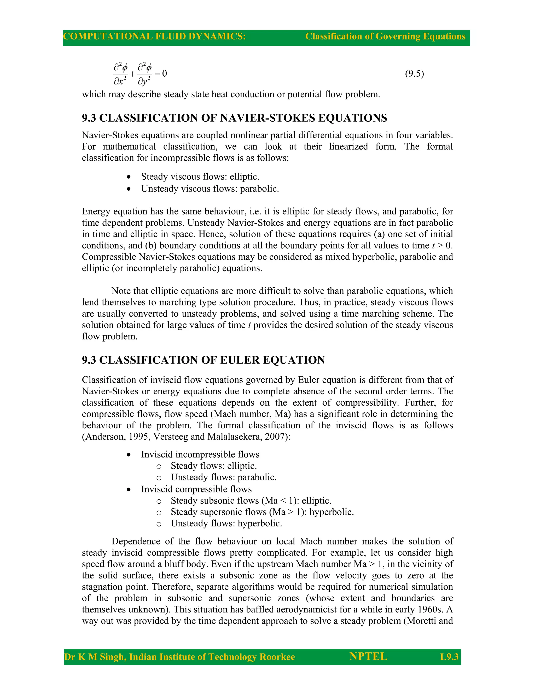
2 2
2 2
0
x y
 
 
 
 
(9.5)
which may describe steady state heat conduction or potential flow problem.
9.3 CLASSIFICATION OF NAVIER-STOKES EQUATIONS
Navier-Stokes equations are coupled nonlinear partial differential equations in four variables.
For mathematical classification, we can look at their linearized form. The formal
classification for incompressible flows is as follows:
 Steady viscous flows: elliptic.
 Unsteady viscous flows: parabolic.
Energy equation has the same behaviour, i.e. it is elliptic for steady flows, and parabolic, for
time dependent problems. Unsteady Navier-Stokes and energy equations are in fact parabolic
in time and elliptic in space. Hence, solution of these equations requires (a) one set of initial
conditions, and (b) boundary conditions at all the boundary points for all values to time t > 0.
Compressible Navier-Stokes equations may be considered as mixed hyperbolic, parabolic and
elliptic (or incompletely parabolic) equations.
Note that elliptic equations are more difficult to solve than parabolic equations, which
lend themselves to marching type solution procedure. Thus, in practice, steady viscous flows
are usually converted to unsteady problems, and solved using a time marching scheme. The
solution obtained for large values of time t provides the desired solution of the steady viscous
flow problem.
9.3 CLASSIFICATION OF EULER EQUATION
Classification of inviscid flow equations governed by Euler equation is different from that of
Navier-Stokes or energy equations due to complete absence of the second order terms. The
classification of these equations depends on the extent of compressibility. Further, for
compressible flows, flow speed (Mach number, Ma) has a significant role in determining the
behaviour of the problem. The formal classification of the inviscid flows is as follows
(Anderson, 1995, Versteeg and Malalasekera, 2007):
 Inviscid incompressible flows
o Steady flows: elliptic.
o Unsteady flows: parabolic.
 Inviscid compressible flows
o Steady subsonic flows (Ma < 1): elliptic.
o Steady supersonic flows (Ma > 1): hyperbolic.
o Unsteady flows: hyperbolic.
Dependence of the flow behaviour on local Mach number makes the solution of
steady inviscid compressible flows pretty complicated. For example, let us consider high
speed flow around a bluff body. Even if the upstream Mach number Ma > 1, in the vicinity of
the solid surface, there exists a subsonic zone as the flow velocity goes to zero at the
stagnation point. Therefore, separate algorithms would be required for numerical simulation
of the problem in subsonic and supersonic zones (whose extent and boundaries are
themselves unknown). This situation has baffled aerodynamicist for a while in early 1960s. A
way out was provided by the time dependent approach to solve a steady problem (Moretti and
COMPUTATIONAL FLUID DYNAMICS: Classification of Governing Equations
Dr K M Singh, Indian Institute of Technology Roorkee NPTEL L9.4
Abbett, 1966), since the unsteady Euler equation for compressible flows is hyperbolic
everywhere (irrespective of the local Mach number). In fact this time dependent approach to
steady state is also widely used now for solution of steady state viscous flows.
REFERENCES
Anderson, J. D., Jr. (1995). Computational Fluid Dynamics: The Basics with Applications.
McGraw Hill, New York.
Ferziger, J. H. And Perić, M. (2003). Computational Methods for Fluid Dynamics. Springer.
Moretti, G. and Abbett, M. (1966). A time-dependent computational method for blunt body
flow. AIAA Journal, 4, 2136-2141.
Versteeg, H. K. and Malalasekera, W. M. G. (2007). Introduction to Computational Fluid
Dynamics: The Finite Volume Method. Second Edition (Indian Reprint) Pearson Education

More Related Content

Similar to Hyperbolic Parabolic & Elliptic systems.pdf

application of differential equation and multiple integral
application of differential equation and multiple integralapplication of differential equation and multiple integral
application of differential equation and multiple integral
divya gupta
 
Conformal Nonlinear Fluid Dynamics from Gravity in Arbitrary Dimensions
Conformal Nonlinear Fluid Dynamics from Gravity in Arbitrary DimensionsConformal Nonlinear Fluid Dynamics from Gravity in Arbitrary Dimensions
Conformal Nonlinear Fluid Dynamics from Gravity in Arbitrary DimensionsMichaelRabinovich
 
Literature survey modeling of microfluidics devices
Literature survey modeling of microfluidics devicesLiterature survey modeling of microfluidics devices
Literature survey modeling of microfluidics devices
Aweshkumarsingh
 
My_Journal_Paper
My_Journal_PaperMy_Journal_Paper
My_Journal_PaperJess Wang
 
E03503025029
E03503025029E03503025029
E03503025029
theijes
 
Effect of Poling Field and Non-linearity in Quantum Breathers in Ferroelectrics
Effect of Poling Field and Non-linearity in Quantum Breathers in FerroelectricsEffect of Poling Field and Non-linearity in Quantum Breathers in Ferroelectrics
Effect of Poling Field and Non-linearity in Quantum Breathers in Ferroelectrics
IOSR Journals
 
Abaqus CFD-Sample Problems
Abaqus CFD-Sample ProblemsAbaqus CFD-Sample Problems
Abaqus CFD-Sample Problems
Andrea Porter
 
Electromagnetic Field Equations
Electromagnetic Field EquationsElectromagnetic Field Equations
Electromagnetic Field Equations
karthikeyanP82
 
6주차
6주차6주차
6주차
Sangho Lee
 
Polarization resistance method
Polarization resistance method Polarization resistance method
Polarization resistance method
justkabe
 
Vol. 1 (1), 2014, 7–11
Vol. 1 (1), 2014, 7–11Vol. 1 (1), 2014, 7–11
Vol. 1 (1), 2014, 7–11
Said Benramache
 
CFD simulation of Lid driven cavity flow
CFD simulation of Lid driven cavity flowCFD simulation of Lid driven cavity flow
CFD simulation of Lid driven cavity flow
IJSRD
 
Stephy index page no 1 to 25 2
Stephy  index page no 1 to 25 2Stephy  index page no 1 to 25 2
Stephy index page no 1 to 25 2
stephy97
 
Electromagnetic Homework Help
Electromagnetic Homework HelpElectromagnetic Homework Help
Electromagnetic Homework Help
Edu Assignment Help
 
Charge Quantization and Magnetic Monopoles
Charge Quantization and Magnetic MonopolesCharge Quantization and Magnetic Monopoles
Charge Quantization and Magnetic Monopoles
Arpan Saha
 
Piyush mahatma sem.2 PPT.pptx
Piyush mahatma sem.2 PPT.pptxPiyush mahatma sem.2 PPT.pptx
Piyush mahatma sem.2 PPT.pptx
PiyushJain242416
 

Similar to Hyperbolic Parabolic & Elliptic systems.pdf (20)

application of differential equation and multiple integral
application of differential equation and multiple integralapplication of differential equation and multiple integral
application of differential equation and multiple integral
 
Conformal Nonlinear Fluid Dynamics from Gravity in Arbitrary Dimensions
Conformal Nonlinear Fluid Dynamics from Gravity in Arbitrary DimensionsConformal Nonlinear Fluid Dynamics from Gravity in Arbitrary Dimensions
Conformal Nonlinear Fluid Dynamics from Gravity in Arbitrary Dimensions
 
Literature survey modeling of microfluidics devices
Literature survey modeling of microfluidics devicesLiterature survey modeling of microfluidics devices
Literature survey modeling of microfluidics devices
 
Dr khalid elhasnaoui 3
Dr khalid elhasnaoui 3Dr khalid elhasnaoui 3
Dr khalid elhasnaoui 3
 
My_Journal_Paper
My_Journal_PaperMy_Journal_Paper
My_Journal_Paper
 
E03503025029
E03503025029E03503025029
E03503025029
 
Effect of Poling Field and Non-linearity in Quantum Breathers in Ferroelectrics
Effect of Poling Field and Non-linearity in Quantum Breathers in FerroelectricsEffect of Poling Field and Non-linearity in Quantum Breathers in Ferroelectrics
Effect of Poling Field and Non-linearity in Quantum Breathers in Ferroelectrics
 
Abaqus CFD-Sample Problems
Abaqus CFD-Sample ProblemsAbaqus CFD-Sample Problems
Abaqus CFD-Sample Problems
 
Electromagnetic Field Equations
Electromagnetic Field EquationsElectromagnetic Field Equations
Electromagnetic Field Equations
 
6주차
6주차6주차
6주차
 
first research paper
first research paperfirst research paper
first research paper
 
03_AJMS_327_21.pdf
03_AJMS_327_21.pdf03_AJMS_327_21.pdf
03_AJMS_327_21.pdf
 
Polarization resistance method
Polarization resistance method Polarization resistance method
Polarization resistance method
 
Vol. 1 (1), 2014, 7–11
Vol. 1 (1), 2014, 7–11Vol. 1 (1), 2014, 7–11
Vol. 1 (1), 2014, 7–11
 
Instantons in 1D QM
Instantons in 1D QMInstantons in 1D QM
Instantons in 1D QM
 
CFD simulation of Lid driven cavity flow
CFD simulation of Lid driven cavity flowCFD simulation of Lid driven cavity flow
CFD simulation of Lid driven cavity flow
 
Stephy index page no 1 to 25 2
Stephy  index page no 1 to 25 2Stephy  index page no 1 to 25 2
Stephy index page no 1 to 25 2
 
Electromagnetic Homework Help
Electromagnetic Homework HelpElectromagnetic Homework Help
Electromagnetic Homework Help
 
Charge Quantization and Magnetic Monopoles
Charge Quantization and Magnetic MonopolesCharge Quantization and Magnetic Monopoles
Charge Quantization and Magnetic Monopoles
 
Piyush mahatma sem.2 PPT.pptx
Piyush mahatma sem.2 PPT.pptxPiyush mahatma sem.2 PPT.pptx
Piyush mahatma sem.2 PPT.pptx
 

Recently uploaded

block diagram and signal flow graph representation
block diagram and signal flow graph representationblock diagram and signal flow graph representation
block diagram and signal flow graph representation
Divya Somashekar
 
MCQ Soil mechanics questions (Soil shear strength).pdf
MCQ Soil mechanics questions (Soil shear strength).pdfMCQ Soil mechanics questions (Soil shear strength).pdf
MCQ Soil mechanics questions (Soil shear strength).pdf
Osamah Alsalih
 
Hybrid optimization of pumped hydro system and solar- Engr. Abdul-Azeez.pdf
Hybrid optimization of pumped hydro system and solar- Engr. Abdul-Azeez.pdfHybrid optimization of pumped hydro system and solar- Engr. Abdul-Azeez.pdf
Hybrid optimization of pumped hydro system and solar- Engr. Abdul-Azeez.pdf
fxintegritypublishin
 
Vaccine management system project report documentation..pdf
Vaccine management system project report documentation..pdfVaccine management system project report documentation..pdf
Vaccine management system project report documentation..pdf
Kamal Acharya
 
H.Seo, ICLR 2024, MLILAB, KAIST AI.pdf
H.Seo,  ICLR 2024, MLILAB,  KAIST AI.pdfH.Seo,  ICLR 2024, MLILAB,  KAIST AI.pdf
H.Seo, ICLR 2024, MLILAB, KAIST AI.pdf
MLILAB
 
Event Management System Vb Net Project Report.pdf
Event Management System Vb Net  Project Report.pdfEvent Management System Vb Net  Project Report.pdf
Event Management System Vb Net Project Report.pdf
Kamal Acharya
 
Architectural Portfolio Sean Lockwood
Architectural Portfolio Sean LockwoodArchitectural Portfolio Sean Lockwood
Architectural Portfolio Sean Lockwood
seandesed
 
Top 10 Oil and Gas Projects in Saudi Arabia 2024.pdf
Top 10 Oil and Gas Projects in Saudi Arabia 2024.pdfTop 10 Oil and Gas Projects in Saudi Arabia 2024.pdf
Top 10 Oil and Gas Projects in Saudi Arabia 2024.pdf
Teleport Manpower Consultant
 
Student information management system project report ii.pdf
Student information management system project report ii.pdfStudent information management system project report ii.pdf
Student information management system project report ii.pdf
Kamal Acharya
 
DESIGN A COTTON SEED SEPARATION MACHINE.docx
DESIGN A COTTON SEED SEPARATION MACHINE.docxDESIGN A COTTON SEED SEPARATION MACHINE.docx
DESIGN A COTTON SEED SEPARATION MACHINE.docx
FluxPrime1
 
WATER CRISIS and its solutions-pptx 1234
WATER CRISIS and its solutions-pptx 1234WATER CRISIS and its solutions-pptx 1234
WATER CRISIS and its solutions-pptx 1234
AafreenAbuthahir2
 
Final project report on grocery store management system..pdf
Final project report on grocery store management system..pdfFinal project report on grocery store management system..pdf
Final project report on grocery store management system..pdf
Kamal Acharya
 
Immunizing Image Classifiers Against Localized Adversary Attacks
Immunizing Image Classifiers Against Localized Adversary AttacksImmunizing Image Classifiers Against Localized Adversary Attacks
Immunizing Image Classifiers Against Localized Adversary Attacks
gerogepatton
 
power quality voltage fluctuation UNIT - I.pptx
power quality voltage fluctuation UNIT - I.pptxpower quality voltage fluctuation UNIT - I.pptx
power quality voltage fluctuation UNIT - I.pptx
ViniHema
 
Railway Signalling Principles Edition 3.pdf
Railway Signalling Principles Edition 3.pdfRailway Signalling Principles Edition 3.pdf
Railway Signalling Principles Edition 3.pdf
TeeVichai
 
addressing modes in computer architecture
addressing modes  in computer architectureaddressing modes  in computer architecture
addressing modes in computer architecture
ShahidSultan24
 
COLLEGE BUS MANAGEMENT SYSTEM PROJECT REPORT.pdf
COLLEGE BUS MANAGEMENT SYSTEM PROJECT REPORT.pdfCOLLEGE BUS MANAGEMENT SYSTEM PROJECT REPORT.pdf
COLLEGE BUS MANAGEMENT SYSTEM PROJECT REPORT.pdf
Kamal Acharya
 
AKS UNIVERSITY Satna Final Year Project By OM Hardaha.pdf
AKS UNIVERSITY Satna Final Year Project By OM Hardaha.pdfAKS UNIVERSITY Satna Final Year Project By OM Hardaha.pdf
AKS UNIVERSITY Satna Final Year Project By OM Hardaha.pdf
SamSarthak3
 
Cosmetic shop management system project report.pdf
Cosmetic shop management system project report.pdfCosmetic shop management system project report.pdf
Cosmetic shop management system project report.pdf
Kamal Acharya
 
weather web application report.pdf
weather web application report.pdfweather web application report.pdf
weather web application report.pdf
Pratik Pawar
 

Recently uploaded (20)

block diagram and signal flow graph representation
block diagram and signal flow graph representationblock diagram and signal flow graph representation
block diagram and signal flow graph representation
 
MCQ Soil mechanics questions (Soil shear strength).pdf
MCQ Soil mechanics questions (Soil shear strength).pdfMCQ Soil mechanics questions (Soil shear strength).pdf
MCQ Soil mechanics questions (Soil shear strength).pdf
 
Hybrid optimization of pumped hydro system and solar- Engr. Abdul-Azeez.pdf
Hybrid optimization of pumped hydro system and solar- Engr. Abdul-Azeez.pdfHybrid optimization of pumped hydro system and solar- Engr. Abdul-Azeez.pdf
Hybrid optimization of pumped hydro system and solar- Engr. Abdul-Azeez.pdf
 
Vaccine management system project report documentation..pdf
Vaccine management system project report documentation..pdfVaccine management system project report documentation..pdf
Vaccine management system project report documentation..pdf
 
H.Seo, ICLR 2024, MLILAB, KAIST AI.pdf
H.Seo,  ICLR 2024, MLILAB,  KAIST AI.pdfH.Seo,  ICLR 2024, MLILAB,  KAIST AI.pdf
H.Seo, ICLR 2024, MLILAB, KAIST AI.pdf
 
Event Management System Vb Net Project Report.pdf
Event Management System Vb Net  Project Report.pdfEvent Management System Vb Net  Project Report.pdf
Event Management System Vb Net Project Report.pdf
 
Architectural Portfolio Sean Lockwood
Architectural Portfolio Sean LockwoodArchitectural Portfolio Sean Lockwood
Architectural Portfolio Sean Lockwood
 
Top 10 Oil and Gas Projects in Saudi Arabia 2024.pdf
Top 10 Oil and Gas Projects in Saudi Arabia 2024.pdfTop 10 Oil and Gas Projects in Saudi Arabia 2024.pdf
Top 10 Oil and Gas Projects in Saudi Arabia 2024.pdf
 
Student information management system project report ii.pdf
Student information management system project report ii.pdfStudent information management system project report ii.pdf
Student information management system project report ii.pdf
 
DESIGN A COTTON SEED SEPARATION MACHINE.docx
DESIGN A COTTON SEED SEPARATION MACHINE.docxDESIGN A COTTON SEED SEPARATION MACHINE.docx
DESIGN A COTTON SEED SEPARATION MACHINE.docx
 
WATER CRISIS and its solutions-pptx 1234
WATER CRISIS and its solutions-pptx 1234WATER CRISIS and its solutions-pptx 1234
WATER CRISIS and its solutions-pptx 1234
 
Final project report on grocery store management system..pdf
Final project report on grocery store management system..pdfFinal project report on grocery store management system..pdf
Final project report on grocery store management system..pdf
 
Immunizing Image Classifiers Against Localized Adversary Attacks
Immunizing Image Classifiers Against Localized Adversary AttacksImmunizing Image Classifiers Against Localized Adversary Attacks
Immunizing Image Classifiers Against Localized Adversary Attacks
 
power quality voltage fluctuation UNIT - I.pptx
power quality voltage fluctuation UNIT - I.pptxpower quality voltage fluctuation UNIT - I.pptx
power quality voltage fluctuation UNIT - I.pptx
 
Railway Signalling Principles Edition 3.pdf
Railway Signalling Principles Edition 3.pdfRailway Signalling Principles Edition 3.pdf
Railway Signalling Principles Edition 3.pdf
 
addressing modes in computer architecture
addressing modes  in computer architectureaddressing modes  in computer architecture
addressing modes in computer architecture
 
COLLEGE BUS MANAGEMENT SYSTEM PROJECT REPORT.pdf
COLLEGE BUS MANAGEMENT SYSTEM PROJECT REPORT.pdfCOLLEGE BUS MANAGEMENT SYSTEM PROJECT REPORT.pdf
COLLEGE BUS MANAGEMENT SYSTEM PROJECT REPORT.pdf
 
AKS UNIVERSITY Satna Final Year Project By OM Hardaha.pdf
AKS UNIVERSITY Satna Final Year Project By OM Hardaha.pdfAKS UNIVERSITY Satna Final Year Project By OM Hardaha.pdf
AKS UNIVERSITY Satna Final Year Project By OM Hardaha.pdf
 
Cosmetic shop management system project report.pdf
Cosmetic shop management system project report.pdfCosmetic shop management system project report.pdf
Cosmetic shop management system project report.pdf
 
weather web application report.pdf
weather web application report.pdfweather web application report.pdf
weather web application report.pdf
 

Hyperbolic Parabolic & Elliptic systems.pdf

  • 1. COMPUTATIONAL FLUID DYNAMICS: Classification of Governing Equations Dr K M Singh, Indian Institute of Technology Roorkee NPTEL L9.1 Lecture 9 CLASSIFICATION OF GOVERNING EQUATIONS 9.1 INTRODUCTION The governing equations of fluid flow (momentum, energy or scalar transport) are second order partial differential equations (PDEs). Choice of the numerical solution technique and number of initial/boundary conditions required for their solution depends on their mathematical character. However, since these equations are system of coupled nonlinear equations in four independent variables (time + three space coordinates), their mathematical classification is rather difficult. Nevertheless, a classification of these equations is usually applied to the linearized form of Navier-Stokes equations. 9.2 CLASSIFICATION OF QUASI-LINEAR PDES Mathematical classification of quasi-linear PDEs is usually based on the classification procedure evolved for a general second order PDE in two independent variables (say, x and y) given by 2 2 2 2 2 0 u u u u u A B C D E Fu G x x y y x y                   (9.1) where A, B, C, D, E, F and G are functions of x and y. Let us assume that 0 A  and 2 4 B AC  is of uniform sign for the range of values of x and y of interest. Classification of PDE (9.1) is based on the type of roots of the associated characteristic equation 2 d d 0 d d y y A B C x x                (9.2) Let ( , ) r x y and ( , ) s x y be the solutions of the preceding equation. Each of these is called a characteristic. Existence of these roots depends on the value of the discriminant 2 4 . B AC  We list in Table 9.1 the type of the PDE for each of the three possible cases. Table 9.1: Classification of quasi-linear second order PDEs Discriminant Nature of characteristics Type of PDE 2 4 0 B AC   Two real characteristics Hyperbolic 2 4 0 B AC   One real characteristic Parabolic 2 4 0 B AC   No real characteristics Elliptic The type name for the PDE has been assigned in analogy with conic sections from analytical geometry wherein the quadratic equation
  • 2. COMPUTATIONAL FLUID DYNAMICS: Classification of Governing Equations Dr K M Singh, Indian Institute of Technology Roorkee NPTEL L9.2 2 2 0 Ax Bxy Cy Dx Ey F       represents a hyperbola if 2 4 0 B AC   , a parabola if 2 4 0 B AC   and an ellipse if 2 4 0 B AC   . The classification of PDE tells us about physical behaviour of the problem. The propagation of information (e.g. effect of disturbance introduced in a flow field) takes place along the characteristics. It also sets the required number of initial/boundary conditions for the given problem. 9.2.1 Hyperbolic Equations In this case, information propagates at a finite speed along the characteristics. Further, any disturbance introduced in the problem domain at a specific point affects the solution in a limited region enclosed within the characteristics through that point. Equations of this type usually appear in time-dependent processes with negligible energy dissipation and lead to wave-type solutions. A typical hyperbolic equation is the wave equation given by 2 2 2 2 2 u u c t x      (9.3) where c denotes the finite speed of wave propagation. The preceding equation requires specification of two sets of initial conditions. 9.2.2 Parabolic Equations Parabolic equations have only one real characteristic. Hence, these require only one set of initial conditions. Further, information travels in only one direction along the characteristic. Thus, these equations lend themselves to marching type solution schemes starting with the given initial data. Parabolic equations usually describe time dependent problems which involve significant amount of diffusion. The typical example is transient heat conduction in a plane wall governed by 2 2 T T t x       (9.4) For the heat diffusion problem (9.4), initial conditions are required at time t = 0. In addition, boundary conditions must be specified at both ends of the wall for all time 0. t  Hence, this problem is also called an initial-boundary value problem. To emphasize the requirement of the boundary conditions, some prefer to classify the transient heat conduction equation (9.4) as parabolic-in-time and elliptic in space. 9.2.3 Elliptic Equations Elliptic equations have no real characteristics. Thus, there is no preferred direction for information propagation, and information travels equally well in all the directions. As a consequence, effect of a disturbance introduced anywhere in the problem domain will be felt everywhere. Thus, one boundary condition is required at all the points on the boundary of the problem domain. Hence, these equations are called boundary-value problems. Elliptic equations usually represent steady state or equilibrium problems (unsteady problems are never elliptic). The representative of the elliptic equation is the Laplace equation given
  • 3. COMPUTATIONAL FLUID DYNAMICS: Classification of Governing Equations Dr K M Singh, Indian Institute of Technology Roorkee NPTEL L9.3 2 2 2 2 0 x y         (9.5) which may describe steady state heat conduction or potential flow problem. 9.3 CLASSIFICATION OF NAVIER-STOKES EQUATIONS Navier-Stokes equations are coupled nonlinear partial differential equations in four variables. For mathematical classification, we can look at their linearized form. The formal classification for incompressible flows is as follows:  Steady viscous flows: elliptic.  Unsteady viscous flows: parabolic. Energy equation has the same behaviour, i.e. it is elliptic for steady flows, and parabolic, for time dependent problems. Unsteady Navier-Stokes and energy equations are in fact parabolic in time and elliptic in space. Hence, solution of these equations requires (a) one set of initial conditions, and (b) boundary conditions at all the boundary points for all values to time t > 0. Compressible Navier-Stokes equations may be considered as mixed hyperbolic, parabolic and elliptic (or incompletely parabolic) equations. Note that elliptic equations are more difficult to solve than parabolic equations, which lend themselves to marching type solution procedure. Thus, in practice, steady viscous flows are usually converted to unsteady problems, and solved using a time marching scheme. The solution obtained for large values of time t provides the desired solution of the steady viscous flow problem. 9.3 CLASSIFICATION OF EULER EQUATION Classification of inviscid flow equations governed by Euler equation is different from that of Navier-Stokes or energy equations due to complete absence of the second order terms. The classification of these equations depends on the extent of compressibility. Further, for compressible flows, flow speed (Mach number, Ma) has a significant role in determining the behaviour of the problem. The formal classification of the inviscid flows is as follows (Anderson, 1995, Versteeg and Malalasekera, 2007):  Inviscid incompressible flows o Steady flows: elliptic. o Unsteady flows: parabolic.  Inviscid compressible flows o Steady subsonic flows (Ma < 1): elliptic. o Steady supersonic flows (Ma > 1): hyperbolic. o Unsteady flows: hyperbolic. Dependence of the flow behaviour on local Mach number makes the solution of steady inviscid compressible flows pretty complicated. For example, let us consider high speed flow around a bluff body. Even if the upstream Mach number Ma > 1, in the vicinity of the solid surface, there exists a subsonic zone as the flow velocity goes to zero at the stagnation point. Therefore, separate algorithms would be required for numerical simulation of the problem in subsonic and supersonic zones (whose extent and boundaries are themselves unknown). This situation has baffled aerodynamicist for a while in early 1960s. A way out was provided by the time dependent approach to solve a steady problem (Moretti and
  • 4. COMPUTATIONAL FLUID DYNAMICS: Classification of Governing Equations Dr K M Singh, Indian Institute of Technology Roorkee NPTEL L9.4 Abbett, 1966), since the unsteady Euler equation for compressible flows is hyperbolic everywhere (irrespective of the local Mach number). In fact this time dependent approach to steady state is also widely used now for solution of steady state viscous flows. REFERENCES Anderson, J. D., Jr. (1995). Computational Fluid Dynamics: The Basics with Applications. McGraw Hill, New York. Ferziger, J. H. And Perić, M. (2003). Computational Methods for Fluid Dynamics. Springer. Moretti, G. and Abbett, M. (1966). A time-dependent computational method for blunt body flow. AIAA Journal, 4, 2136-2141. Versteeg, H. K. and Malalasekera, W. M. G. (2007). Introduction to Computational Fluid Dynamics: The Finite Volume Method. Second Edition (Indian Reprint) Pearson Education