Researchers at Georgia Institute of Technology are addressing helicopter blade-vortex interaction (BVI) using computational methods to improve helicopter performance and reduce noise. The study examines the effectiveness of passive devices (spoilers) placed near the rotor tips to diffuse tip vortices, which could lead to enhanced efficiency and decreased maintenance costs. The methodology involves complex simulations that have been validated against experimental data, demonstrating promising results in vortex diffusion.

1. Computational Investigation of
Helicopter Rotor Tip Vortex Diffusion
Using Passive Tip Devices
L.N. Sankar, Professor
Justin W. Russell, Graduate Research Assistant
School of Aerospace Engineering
Georgia Institute of Technology
Atlanta, GA 30332−0150
(404) 894−3014
Michael T. Patterson, Systems Engineer
DoD High Performance Computing
Silicon Graphics / Cray Research, Inc.
Peachtree City, GA 30269
(770) 631−2243
Researchers at the Georgia Institute of Technology in Atlanta, Georgia are using DoD HPCMP
computer equipment to solve helicopter aerodynamics problems. One such problem is the
blade−vortex interaction (BVI) problem. As a helicopter flies, its blades produce vortices which
interact with subsequently passing blades. This interaction limits a helicopter’s performance, vibrates
the rotor and fuselage, fatigues the entire aircraft, and creates noise which can be heard for great
distances. Solutions to and an understanding of the helicopter BVI problem can improve
performance, reduce maintenance costs, increase reliability, and benefit public perception of
helicopters.
Current solution methodologies which model the helicopter BVI problem require tens or hundreds of
Cray computing hours and can generate tens of gigabytes of data. Computation and storage of the
aerodynamics solution requires high performance hardware and software, and reliable data
management techniques. Examination of gigabytes of solution data requires graphical techniques.
The DoD HPCMP is providing the computer resources necessary to solve such problems.
Methodology
In the present BVI study, a two−bladed NASA test rotor is embedded in a computational grid as
shown in Figure (1). In this figure, only one blade of the rotor is shown, and only the lower half of
the grid is shown. The blade is colored grey. In this figure, the observer is stationed above the rotor.
The helicopter fuselage, which would be below the rotor, has not been included in the study. This
test rotor is 7.5 feet in diameter, and each blade’s chord length is 7.5 inches.
Table 1. Dimensions for the Three Spoilers
Spoiler Height Width Location
Number (% chord) (%radius) (% radius)
1 3.9 5.8 87.5 − 93.3
2 5.0 8.8 85.6 − 94.4
3 8.4 13.3 83.5 − 96.8
For the hovering cases examined in
this study, each of the two blades
encounters and produces the same
flow field. Thus a solution can be
obtained more econically by
solving for the flow field over only
one blade, and applying periodic
boundary conditions to simulate
the presence of the second blade,

2. Figure 1. One Blade of a Two−bladed NASA Test Rotor
Embedded in a Computational Grid.
Figure 2. The NASA Test Rotor Vortex Field. Rotor
Blades are Colored Grey, Vortex Sheets Blue, and the Tip
Vortices are Colored by the Fluid Velocity Magnitude.
which will be shown in many of
the subsequent figures. The
computational grid about one
blade is an eight−zone
structured H−H−O topology and
consists of 1.2 million points.
The numerical solution
employed in this study is fifth
order accurate in space and first
order accurate in time. The
solver uses a cell−vertex finite
volume scheme in which the
fluid fluxes crossing cell faces
are computed using Roe’s
approximate Riemann solver.
Air turbulence is simulated with
the algebraic Baldwin−Lomax
eddy viscosity model.
Boundary conditions for the
flow variables at the
computational domain’s far field
boundaries are implemented
with high−order extrapolations.
The complete solution
methodology is presented in
Ref. [1].
Results
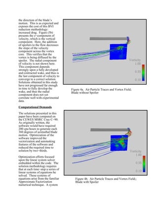
Figure (2) presents a computed
tip vortex for the NASA test
rotor in hover. In this figure, the
rotor is again viewed from
above. The rotor is moving in
the counter−clockwise direction
at 550 rpm. Computed velocity
components within the vortex
core have been validated against
NASA experimental data
adquired by laser−velicometer
techniques. The computed
solution has been found to
adequately model the vortex.
Ref. [2] examines the
correlation of the present data
with the NASA experimental
data in detail.
The objective of this work is to
diffuse the tip vortex by placing
a spoiler (a tab) at the blade’s
trailing edge near the blade tip.
Analytical studies have

3. Figure 3b. Air Particle Traces Colored by the Fluid
Vorticity Magnitude; Blade with Spoiler
Figure 3a. Air Particle Traces Colored by the Fluid
Vorticity Magnitude; Blade without Spoiler
suggested the feasibility of this
approach to reducing BVI. Three
spoilers have been tested in this
study: their dimensions are
presented in Table (1). In
subsequent figures, only the clean
rotor (which has no spoiler) and
the rotor with the largest spoiler
will be shown for brevity.
Figures (3a) and (3b) present
computed particle traces which
emanate from the blade tip’s
leading edge. The effect of the
spoiler is apparent in Figure (3b):
particle traces through the
spoiler’s flow field diverge,
indicating tip vortex diffusion.
Figures (4a) and (4b) present the
particle traces again, and also the
vorticity field on a plane three
chordlengths behind the blade.
The diffused vortex field of the
spoiler is evident. In the diffused
field three tip vorticies are
present: the first vortex resides
highest in the figure, and is the
usual tip vortex. Compared to the
clean rotor tip vortex, the tip
vortex in Figure (4b) has a
reduced magnitude, as desired.
The second vortex, lowest in
Figure (4b), originates at the
outboard edge of the spoiler. The
third vortex originates at the
spoiler’s inboard edge: this vortex
rotates in the opposite direction
of the other two vortices, and
although smaller in magnitude
than the other two vorticies,
critically aids the diffusion
process.
Figures (5a) and (5b) present
computed velocity components
along the radial (y) direction of
the vortex core, again three
chordlengths downstream from
the blade. The x−component of
fluid velocity is the chord−wise
component: addition of spoilers
to the flow field increases this
component, indicating that fluid
is being more strongly dragged in

4. Figure 4a. Air Particle Traces and Vortex Field;
Blade without Spoiler
Figure 4b. Air Particle Traces and Vortex Field;;
Blade with Spoiler
the direction of the blade’s
motion. This is as expected and
exposes the cost of this BVI
reduction methodology:
increased drag. Figure (5b)
presents the z−component of
velocity, which is the vertical
component. Here, the addition
of spoilers to the flow decreases
the slope of the velocity
component across the vortex
core. This verifies that the
vortex is being diffused by the
spoiler. The radial component
of velocity is not shown here.
This component depends
strongly upon a fully developed
and contracted wake, and thus is
the last component of velocity to
converge to a correct solution.
Solutions obtained in this study
have not progressed far enough
in time to fully develop the
wake, and thus the radial
component does not yet
correlate well with experimental
data.
Computational Demands
The solutions presented in this
paper have been computed on
the CEWES MSRC Cray C−90.
As originally written, the
software would have required
200 cpu hours to generate each
360 degrees of azimuthal blade
motion. Optimization of the
software improved the
vectorization and autotasking
features of the software and
reduced the required time to
solution by two−thirds.
Optimization efforts focused
upon the linear system solver
embedded within the code. The
solution methodology requires
that at each time−step a series of
linear systems of equations be
solved. These systems of
equations arise from the familiar
Approximate Factorization
numerical technique. A system

5. Figure 5a. Comparison of Vortex Core X−velocity
Component with and without Spoiler
Figure 5b. Comparison of Vortex Core Z−velocity
Component with and without Spoiler
of equations must therefore be
solved for the five flow variables
along each line of the grid: that
is, along each ξ−line, each
η−line, and each ζ−line.
Written for scalar machines, this
part of the software was
constructed to minimize memory
usage by working sequentially
on each system of equations.
For this study, the software was
modified to attack all solutions
simultaneously, at the expense
of a modest amount of additional
required memory.
Most recently, the software has
been ported to a Silicon
Graphics Origin 2000, where
continuing studies are being
conducted.
Acknowledgements
The authors wish to express
thanks to the National Rotorcraft
Technology Center for their
support of this project as part of
the Georgia Tech Rotorcraft
Center of Excellence. The
authors also wish to thank Chee
Tung of the Army
Aeroflightdynamics Directorate,
NASA Ames, for his
contributions to this work.
References
1. Hariharan, N., "High Order
Simulation of Unsteady
Compressible Flows Over
Interacting Bodies with Overset
Grids," Ph.D. Thesis, Georgia
Institute of Technology, Atlanta,
GA, August 1995.
2. Russell, J., et al., "Alterations
of the Tip Vortex Structure from
a Hovering Rotor using Passive
Tip Devices," American
Helicopter Society Forum, April
29 − May 1, 1997.