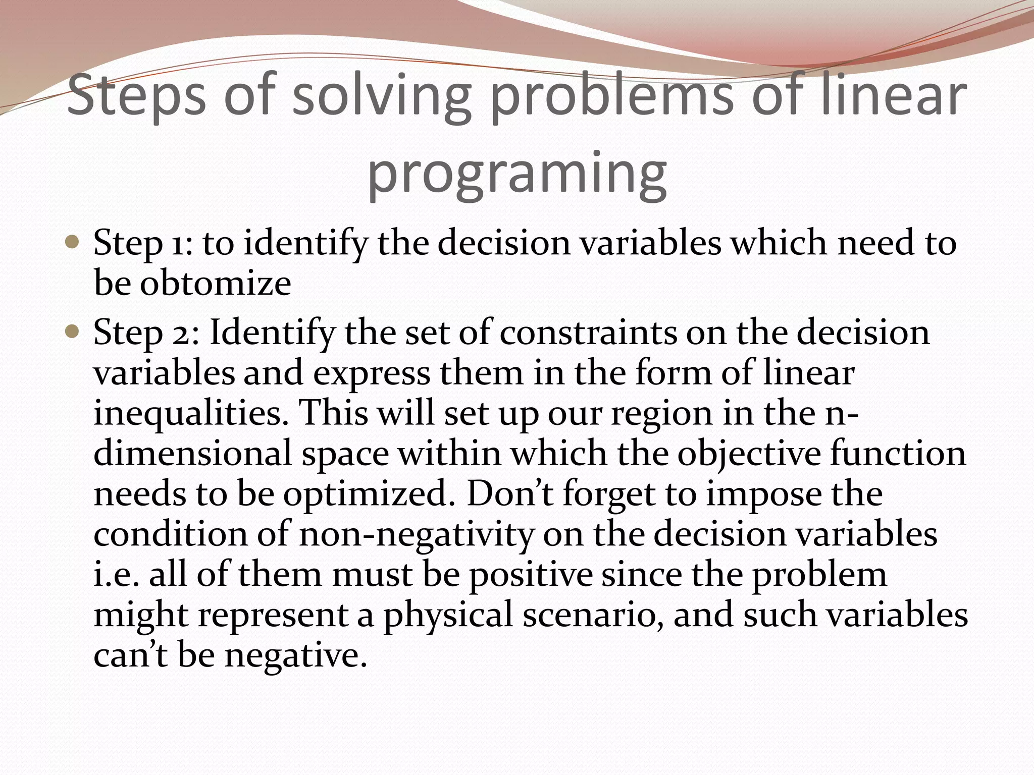
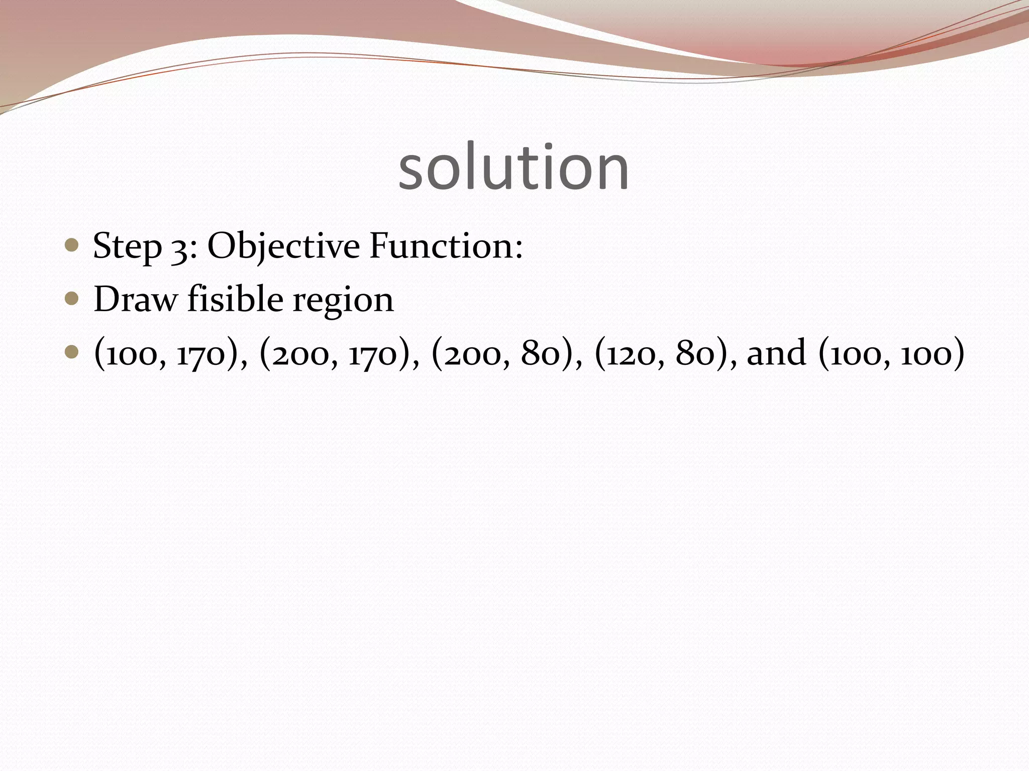
Syeda Shajiah zahra zaidi 14
Amna nazir 59
Muazma nageen 06
Muqadas fatima 22
Adeera wasiq 20
Linear programing
History
 in 1939 linear
programming was
developed by Leonid
Kantorovich
 During world war 2
 To decrease loss and cost
on army and to increase
loss of enemies
Definition
 “Linear programming is a mathematical method that
is used to determine the best possible outcome or
solution from a given set of parameters or list of
requirements, which are represented in the form of
linear relationships.”
Steps of solving problems of linear
programing
 Step 1: to identify the decision variables which need to
be obtomize
 Step 2: Identify the set of constraints on the decision
variables and express them in the form of linear
inequalities. This will set up our region in the n-
dimensional space within which the objective function
needs to be optimized. Don’t forget to impose the
condition of non-negativity on the decision variables
i.e. all of them must be positive since the problem
might represent a physical scenario, and such variables
can’t be negative.
Steps of solving problems of linear
programing
 Step 3:Express the objective function in the form of
a linear equation in the decision variables.
 Step 4:Optimize the objective function
either graphically or mathematically.
Example
Question
calculator company produces a scientific calculator and a graphing
calculator. Long-term projections indicate an expected demand of at
least 100 scientific and 80 graphing calculators each day. Because of
limitations on production capacity, no more than 200 scientific
and 170 graphing calculators can be made daily. To satisfy a shipping
contract, a total of at least 200 calculators much be shipped each day.
If each scientific calculator sold results in a $2 loss, but each graphing
calculator produces a $5 profit, how many of each type should be made
daily to maximize net profits?
solution
 Step 1: The decision variables
 Since the question has asked for an optimum number
of calculators, that’s what our decision variables in this
problem would be. Let,
 x = number of scientific calculators produced
y = number of graphing calculators produced
Solution
 Step 2: The constraints
 Since the company can’t produce a negative number of
calculators in a day, a natural constraint would be:
 x ≥ 0,y ≥ 0
 P = –2x + 5y, subject to:
 100 < x < 200
80 < y < 170
y > –x + 200
solution
 Step 3: Objective Function:
 Draw fisible region
 (100, 170), (200, 170), (200, 80), (120, 80), and (100, 100)
solution
 Step 4: optimize the objective function now
 Put all the corner points in the function
 P = –2x + 5y
Limitations of linear programing
 For large problems the computational difficulties are
enormous.
 It may yield fractional value answers to decision
variables.
 It is applicable to only static situation.
 linear programing deals with the problems with single
objective
Applications of the linear
programoing
 Transportation systems rely upon linear programming
for cost and time efficiency. Bus and train routes must
factor in scheduling, travel time and passengers.
 Airlines use linear programming to optimize their
profits according to different seat prices and customer
demand. Airlines also use linear programming for pilot
scheduling and routes. Optimization via linear
programming increases airlines' efficiency and
decreases expenses.
Group members

Group members

  • 1.
    Syeda Shajiah zahrazaidi 14 Amna nazir 59 Muazma nageen 06 Muqadas fatima 22 Adeera wasiq 20
  • 2.
  • 3.
    History  in 1939linear programming was developed by Leonid Kantorovich  During world war 2  To decrease loss and cost on army and to increase loss of enemies
  • 4.
    Definition  “Linear programmingis a mathematical method that is used to determine the best possible outcome or solution from a given set of parameters or list of requirements, which are represented in the form of linear relationships.”
  • 5.
    Steps of solvingproblems of linear programing  Step 1: to identify the decision variables which need to be obtomize  Step 2: Identify the set of constraints on the decision variables and express them in the form of linear inequalities. This will set up our region in the n- dimensional space within which the objective function needs to be optimized. Don’t forget to impose the condition of non-negativity on the decision variables i.e. all of them must be positive since the problem might represent a physical scenario, and such variables can’t be negative.
  • 6.
    Steps of solvingproblems of linear programing  Step 3:Express the objective function in the form of a linear equation in the decision variables.  Step 4:Optimize the objective function either graphically or mathematically.
  • 7.
    Example Question calculator company producesa scientific calculator and a graphing calculator. Long-term projections indicate an expected demand of at least 100 scientific and 80 graphing calculators each day. Because of limitations on production capacity, no more than 200 scientific and 170 graphing calculators can be made daily. To satisfy a shipping contract, a total of at least 200 calculators much be shipped each day. If each scientific calculator sold results in a $2 loss, but each graphing calculator produces a $5 profit, how many of each type should be made daily to maximize net profits?
  • 8.
    solution  Step 1:The decision variables  Since the question has asked for an optimum number of calculators, that’s what our decision variables in this problem would be. Let,  x = number of scientific calculators produced y = number of graphing calculators produced
  • 9.
    Solution  Step 2:The constraints  Since the company can’t produce a negative number of calculators in a day, a natural constraint would be:  x ≥ 0,y ≥ 0  P = –2x + 5y, subject to:  100 < x < 200 80 < y < 170 y > –x + 200
  • 10.
    solution  Step 3:Objective Function:  Draw fisible region  (100, 170), (200, 170), (200, 80), (120, 80), and (100, 100)
  • 11.
    solution  Step 4:optimize the objective function now  Put all the corner points in the function  P = –2x + 5y
  • 12.
    Limitations of linearprograming  For large problems the computational difficulties are enormous.  It may yield fractional value answers to decision variables.  It is applicable to only static situation.  linear programing deals with the problems with single objective
  • 13.
    Applications of thelinear programoing  Transportation systems rely upon linear programming for cost and time efficiency. Bus and train routes must factor in scheduling, travel time and passengers.  Airlines use linear programming to optimize their profits according to different seat prices and customer demand. Airlines also use linear programming for pilot scheduling and routes. Optimization via linear programming increases airlines' efficiency and decreases expenses.