Graphs data structure

1. CHAPTER 6 1
CHAPTER 6
GRAPHS
All the programs in this file are selected from
Ellis Horowitz, Sartaj Sahni, and Susan Anderson-Freed
“Fundamentals of Data Structures in C”,
Computer Science Press, 1992.

2. Introduction
 First Recorded evidence – 1736 – Leonhard
Euler – solve classical – Konigsberg bridge
problem.
 4 Land areas (A to D) – isolated by river.
 Interconnected by 7 bridges ( a to g).
 Problem: start at one land location – is it
possible to walk across all bridges exactly
once and reach the starting land area?
2

3. Introduction
3

4. Intro…..
 Leonhard’s solution:
 Start from Land area B
 Walk across bridge a to island A
 Take bridge e to area D
 Take bridge g to C
 Take bridge b to B
 Take bridge f to D
 Wrong !!! – Euler answered in negative – Not
possible
4

5. Intro….
 Euler – represented – land area – vertex – bridges –
edges.
 Degree of a vertex – number of edges incident on it.
 A walk starting at vertex – going through each
edge exactly once – terminating at starting
vertex – possible – iff – the degrees of each
vertex is even.
 A walk that does this is called as Eulerian.
 No Eulerian walk – Konigsberg Bridge problem
5

6. Applications…….
 Analysis of electric circuits.
 Finding shortest routes.
 Project planning.
 Identification of chemical compounds.
 Statistical Mechanics.
 Genetics
 Cybernetics
 Linguistics
 Social Sciences
6

7. 7
Definition
 A graph G consists of two sets
– a finite, nonempty set of vertices V(G)
– a finite, possible empty set of edges E(G)
– G(V,E) represents a graph
 An undirected graph is one in which the pair of
vertices in a edge is unordered, (v0, v1) = (v1,v0)
 A directed graph is one in which each edge is a
directed pair of vertices, <v0, v1> != <v1,v0>
tail head

8. 8
Examples for Graph
0
1 2
3
0
1
2
0
1 2
3 4 5 6
G1
G2
G3
V(G1)={0,1,2,3} E(G1)={(0,1),(0,2),(0,3),(1,2),(1,3),(2,3)}
V(G2)={0,1,2,3,4,5,6} E(G2)={(0,1),(0,2),(1,3),(1,4),(2,5),(2,6)}
V(G3)={0,1,2} E(G3)={<0,1>,<1,0>,<1,2>}
complete undirected graph: n(n-1)/2 edges
complete directed graph: n(n-1) edges
complete graph incomplete graph

9. 9
Complete Graph
 A complete graph is a graph that has the
maximum number of edges
– for undirected graph with n vertices, the maximum
number of edges is n(n-1)/2
– for directed graph with n vertices, the maximum
number of edges is n(n-1)
– example: G1 is a complete graph

10. 10
Adjacent and Incident
 If (v0, v1) is an edge in an undirected graph,
– v0 and v1 are adjacent
– The edge (v0, v1) is incident on vertices v0 and v1
 If <v0, v1> is an edge in a directed graph
– v0 is adjacent to v1, and v1 is adjacent from v0
– The edge <v0, v1> is incident on v0 and v1

11. CHAPTER 6 11
0 2
1
(a)
2
1
0
3
(b)
*Figure 6.3:Example of a graph with feedback loops and a
multigraph (p.260)
self edge multigraph:
multiple occurrences
of the same edge
Figure 6.3

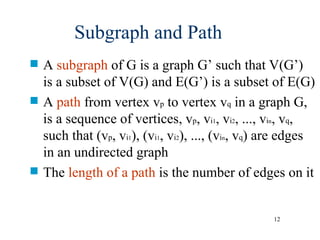
12. 12
 A subgraph of G is a graph G’ such that V(G’)
is a subset of V(G) and E(G’) is a subset of E(G)
 A path from vertex vp to vertex vq in a graph G,
is a sequence of vertices, vp, vi1, vi2, ..., vin, vq,
such that (vp, vi1), (vi1, vi2), ..., (vin, vq) are edges
in an undirected graph
 The length of a path is the number of edges on it
Subgraph and Path

13. 13
0 0
1 2 3
1 2 0
1 2
3
(i) (ii) (iii) (iv)
(a) Some of the subgraph of G1
0 0
1
0
1
2
0
1
2
(i) (ii) (iii) (iv)
(b) Some of the subgraph of G3
0
1 2
3
G1
0
1
2
G3
Figure 6.4: subgraphs of G1 and G3 (p.261)

14. 14
 A simple path is a path in which all vertices,
except possibly the first and the last, are distinct
 A cycle is a simple path in which the first and
the last vertices are the same
 In an undirected graph G, two vertices, v0 and v1, are
connected if there is a path in G from v0 to v1
 An undirected graph is connected if, for every
pair of distinct vertices vi, vj, there is a path
from vi to vj
Simple Path and Style

15. 15
0
1 2
3
0
1 2
3 4 5 6
G1
G2
connected
tree (acyclic graph)

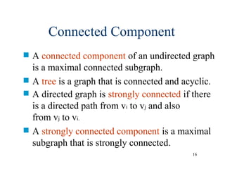
16. 16
 A connected component of an undirected graph
is a maximal connected subgraph.
 A tree is a graph that is connected and acyclic.
 A directed graph is strongly connected if there
is a directed path from vi to vj and also
from vj to vi.
 A strongly connected component is a maximal
subgraph that is strongly connected.
Connected Component

17. 17
*Figure 6.5: A graph with two connected components (p.262)
1
0
2
3
4
5
6
7
H1
H2
G4 (not connected)
connected component (maximal connected subgraph)

18. CHAPTER 6 18
*Figure 6.6: Strongly connected components of G3 (p.262)
0
1
2
0
1
2
G3
not strongly connected
strongly connected component
(maximal strongly connected subgraph)

19. CHAPTER 6 19
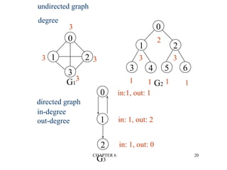
Degree
 The degree of a vertex is the number of edges
incident to that vertex
 For directed graph,
– the in-degree of a vertex v is the number of edges
that have v as the head
– the out-degree of a vertex v is the number of edges
that have v as the tail
– if di is the degree of a vertex i in a graph G with n
vertices and e edges, the number of edges is
e di
n



( ) /
0
1
2

20. CHAPTER 6 20
undirected graph
degree
0
1 2
3 4 5 6
G1 G2
3
2
3 3
1 1 1 1
directed graph
in-degree
out-degree
0
1
2
G3
in:1, out: 1
in: 1, out: 2
in: 1, out: 0
0
1 2
3
3
3
3

21. CHAPTER 6 21
ADT for Graph
structure Graph is
objects: a nonempty set of vertices and a set of undirected edges, where each
edge is a pair of vertices
functions: for all graph  Graph, v, v1 and v2  Vertices
Graph Create()::=return an empty graph
Graph InsertVertex(graph, v)::= return a graph with v inserted. v has no
incident edge.
Graph InsertEdge(graph, v1,v2)::= return a graph with new edge
between v1 and v2
Graph DeleteVertex(graph, v)::= return a graph in which v and all edges
incident to it are removed
Graph DeleteEdge(graph, v1, v2)::=return a graph in which the edge (v1, v2)
is removed
Boolean IsEmpty(graph)::= if (graph==empty graph) return TRUE
else return FALSE
List Adjacent(graph,v)::= return a list of all vertices that are adjacent to v

22. CHAPTER 6 22
Graph Representations
 Adjacency Matrix
 Adjacency Lists
 Adjacency Multilists

23. CHAPTER 6 23
Adjacency Matrix
 Let G=(V,E) be a graph with n vertices.
 The adjacency matrix of G is a two-dimensional
n by n array, say adj_mat
 If the edge (vi, vj) is in E(G), adj_mat[i][j]=1
 If there is no such edge in E(G), adj_mat[i][j]=0
 The adjacency matrix for an undirected graph is
symmetric; the adjacency matrix for a digraph
need not be symmetric

24. CHAPTER 6 24
Examples for Adjacency Matrix
0
1
1
1
1
0
1
1
1
1
0
1
1
1
1
0












0
1
0
1
0
0
0
1
0










0
1
1
0
0
0
0
0
1
0
0
1
0
0
0
0
1
0
0
1
0
0
0
0
0
1
1
0
0
0
0
0
0
0
0
0
0
1
0
0
0
0
0
0
1
0
1
0
0
0
0
0
0
1
0
1
0
0
0
0
0
0
1
0


























G1
G2
G4
0
1 2
3
0
1
2
1
0
2
3
4
5
6
7
symmetric
undirected: n2
/2
directed: n2

25. CHAPTER 6 25
Merits of Adjacency Matrix
 From the adjacency matrix, to determine the
connection of vertices is easy
 The degree of a vertex is
 For a digraph, the row sum is the out_degree,
while the column sum is the in_degree
adj mat i j
j
n
_ [ ][ ]



0
1
ind vi A j i
j
n
( ) [ , ]




0
1
outd vi A i j
j
n
( ) [ , ]




0
1

26. CHAPTER 6 26
Data Structures for Adjacency Lists
#define MAX_VERTICES 50
typedef struct node *node_pointer;
typedef struct node {
int vertex;
struct node *link;
};
node_pointer graph[MAX_VERTICES];
int n=0; /* vertices currently in use *
Each row in adjacency matrix is represented as an adjacency list.

27. CHAPTER 6 27
0
1
2
3
0
1
2
0
1
2
3
4
5
6
7
1 2 3
0 2 3
0 1 3
0 1 2
G1
1
0 2
G3
1 2
0 3
0 3
1 2
5
4 6
5 7
6
G4
0
1 2
3
0
1
2
1
0
2
3
4
5
6
7
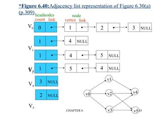
An undirected graph with n vertices and e edges ==> n head nodes and 2e list nodes

28. CHAPTER 6 28
 3  2 NULL
1 
0
 2  3 NULL
0 
1
 3  1 NULL
0 
2
 2  0 NULL
1 
3
headnodes vertax link
Order is of no significance.
0
1 2
3
Figure 6.13:Alternate order adjacency list for G1 (p.268)

29. CHAPTER 6 29
Interesting Operations
degree of a vertex in an undirected graph
–# of nodes in adjacency list
# of edges in a graph
–determined in O(n+e)
out-degree of a vertex in a directed graph
–# of nodes in its adjacency list
in-degree of a vertex in a directed graph
–traverse the whole data structure

30. CHAPTER 6 30
[0] 9 [8] 23 [16] 2
[1] 11 [9] 1 [17] 5
[2] 13 [10] 2 [18] 4
[3] 15 [11] 0 [19] 6
[4] 17 [12] 3 [20] 5
[5] 18 [13] 0 [21] 7
[6] 20 [14] 3 [22] 6
[7] 22 [15] 1
1
0
2
3
4
5
6
7
0
1
2
3
4
5
6
7
node[0] … node[n-1]: starting point for vertices
node[n]: n+2e+1
node[n+1] … node[n+2e]: head node of edge
Compact Representation

31. CHAPTER 6 31



0
1
2
1 NULL
0 NULL
1 NULL
0
1
2
Determine in-degree of a vertex in a fast way.
Figure 6.10: Inverse adjacency list for G3

32. CHAPTER 6 32
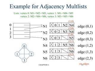
Adjacency Multilists
marked vertex1 vertex2 path1 path2
An edge in an undirected graph is
represented by two nodes in adjacency list
representation.
Adjacency Multilists
–lists in which nodes may be shared among
several lists.
(an edge is shared by two different paths)

33. CHAPTER 6 33
0 1 N2 N4
0 2 N3 N4
0 3 N5
1 2 N5 N6
1 3 N6
2 3
N1
N2
N3
N4
N5
N6
0
1
2
3
edge (0,1)
edge (0,2)
edge (0,3)
edge (1,2)
edge (1,3)
edge (2,3)
(1,0)
(2,0)
(3,0)
(2,1)
(3,1)
(3,2)
0
1 2
3
six edges
Lists: vertex 0: M1->M2->M3, vertex 1: M1->M4->M5
vertex 2: M2->M4->M6, vertex 3: M3->M5->M6
Example for Adjacency Multlists

34. CHAPTER 6 34
typedef struct edge *edge_pointer;
typedef struct edge {
short int marked;
int vertex1, vertex2;
edge_pointer path1, path2;
};
edge_pointer graph[MAX_VERTICES];
marked vertex1 vertex2 path1 path2
Adjacency Multilists

35. CHAPTER 6 35
Some Graph Operations
 Traversal
Given G=(V,E) and vertex v, find all wV,
such that w connects v.
– Depth First Search (DFS)
preorder tree traversal
– Breadth First Search (BFS)
level order tree traversal
 Connected Components
 Spanning Trees

36. CHAPTER 6 36
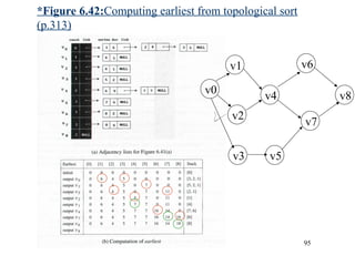
*Figure 6.19:Graph G and its adjacency lists (p.274)
depth first search: v0, v1, v3, v7, v4, v5, v2, v6
breadth first search: v0, v1, v2, v3, v4, v5, v6, v7
Vertex Visit
0 0
1 0
2 0
3 0
4 0
5 0
6 0
7 0

37. CHAPTER 6 37
Depth First Search
void dfs(int v)
{
node_pointer w;
visited[v]= TRUE;
printf(“%5d”, v);
for (w=graph[v]; w; w=w->link)
if (!visited[w->vertex])
dfs(w->vertex);
}
#define FALSE 0
#define TRUE 1
short int visited[MAX_VERTICES];
Data structure
adjacency list: O(e)
adjacency matrix: O(n2
)

38. CHAPTER 6 38
Breadth First Search
typedef struct queue *queue_pointer;
typedef struct queue {
int vertex;
queue_pointer link;
};
void addq(queue_pointer *,
queue_pointer *, int);
int deleteq(queue_pointer *);

39. CHAPTER 6 39
Breadth First Search (Continued)
void bfs(int v)
{
node_pointer w;
queue_pointer front, rear;
front = rear = NULL;
printf(“%5d”, v);
visited[v] = TRUE;
addq(&front, &rear, v);
adjacency list: O(e)
adjacency matrix: O(n2
)

40. CHAPTER 6 40
while (front) {
v= deleteq(&front);
for (w=graph[v]; w; w=w->link)
if (!visited[w->vertex]) {
printf(“%5d”, w->vertex);
addq(&front, &rear, w->vertex);
visited[w->vertex] = TRUE;
}
}
}

41. CHAPTER 6 41
Connected Components
void connected(void)
{
for (i=0; i<n; i++) {
if (!visited[i]) {
dfs(i);
printf(“n”);
}
}
}
adjacency list: O(n+e)
adjacency matrix: O(n2
)

42. CHAPTER 6 42
Spanning Trees
 When graph G is connected, a depth first or
breadth first search starting at any vertex will
visit all vertices in G
 A spanning tree is any tree that consists solely
of edges in G and that includes all the vertices
 E(G): T (tree edges) + N (nontree edges)
where T: set of edges used during search
N: set of remaining edges

43. CHAPTER 6 43
Examples of Spanning Tree
0
1 2
3
0
1 2
3
0
1 2
3
0
1 2
3
G1 Possible spanning trees

44. CHAPTER 6 44
Spanning Trees
 Either dfs or bfs can be used to create a
spanning tree
– When dfs is used, the resulting spanning tree is
known as a depth first spanning tree
– When bfs is used, the resulting spanning tree is
known as a breadth first spanning tree
 While adding a nontree edge into any spanning
tree, this will create a cycle

45. CHAPTER 6 45
DFS VS BFS Spanning Tree
0
1 2
3 4 5 6
7
0
1 2
3 4 5 6
7
DFS Spanning BFS Spanning
0
1 2
3 4 5 6
7 nontree edge
cycle

46. CHAPTER 6 46
Minimum Cost Spanning Tree
 The cost of a spanning tree of a weighted
undirected graph is the sum of the costs of the
edges in the spanning tree
 A minimum cost spanning tree is a spanning
tree of least cost
 Three different algorithms can be used
– Kruskal
– Prim
– Sollin
Select n-1 edges from a weighted graph
of n vertices with minimum cost.

47. CHAPTER 6 47
Greedy Strategy
 An optimal solution is constructed in stages
 At each stage, the best decision is made at this
time
 Since this decision cannot be changed later,
we make sure that the decision will result in a feasib
solution
 Typically, the selection of an item at each
stage is based on a least cost or a highest profit crite

48. CHAPTER 6 48
Kruskal’s Idea
 Build a minimum cost spanning tree T by
adding edges to T one at a time
 Select the edges for inclusion in T in
nondecreasing order of the cost
 An edge is added to T if it does not form a
cycle
 Since G is connected and has n > 0 vertices,
exactly n-1 edges will be selected

49. CHAPTER 6 49
Examples for Kruskal’s Algorithm
0
1
2
3
4
5 6
0
1
2
3
4
5 6
28
16
12
18
24
22
25
10
14
0
1
2
3
4
5 6
10
0 5
2 3
1 6
1 2
3 6
3 4
4 6
4 5
10
12
14
16
18
22
24
25
28
6/9

50. CHAPTER 6 50
0
1
2
3
4
5 6
10
12
0
1
2
3
4
5 6
10
12
14
0
1
2
3
4
5 6
10
12
14 16
0 5
2 3
1 6
1 2
3 6
3 4
4 6
4 5
0 1
10
12
14
16
18
22
24
25
28 + 3 6
cycle

51. CHAPTER 6 51
0 5
2 3
1 6
1 2
3 6
3 4
4 6
4 5
0 1
10
12
14
16
18
22
24
25
28
0
1
2
3
4
5 6
10
12
14 16
22
0
1
2
3
4
5 6
10
12
14 16
22
25
4 6
cycle
+
cost = 10 +25+22+12+16+14

52. CHAPTER 6 52
Kruskal’s Algorithm
T= {};
while (T contains less than n-1 edges
&& E is not empty) {
choose a least cost edge (v,w) from E;
delete (v,w) from E;
if ((v,w) does not create a cycle in T)
add (v,w) to T
else discard (v,w);
}
if (T contains fewer than n-1 edges)
printf(“No spanning treen”);
O(e log e)

53. CHAPTER 6 53
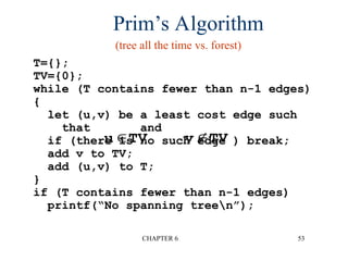
Prim’s Algorithm
T={};
TV={0};
while (T contains fewer than n-1 edges)
{
let (u,v) be a least cost edge such
that and
if (there is no such edge ) break;
add v to TV;
add (u,v) to T;
}
if (T contains fewer than n-1 edges)
printf(“No spanning treen”);
u TV
 v TV

(tree all the time vs. forest)

54. CHAPTER 6 54
Examples for Prim’s Algorithm
0
1
2
3
4
5 6
0
1
2
3
4
5 6
10
0
1
2
3
4
5 6
10
10
25 25
22
0
1
2
3
4
5 6
28
16
12
18
24
22
25
10
14

55. CHAPTER 6 55
0
1
2
3
4
5 6
10
25
22
12
0
1
2
3
4
5 6
10
25
22
12
16
0
1
2
3
4
5 6
10
25
22
12
16
14
0
1
2
3
4
5 6
28
16
12
18
24
22
25
10
14

56. CHAPTER 6 56
Sollin’s Algorithm
0
1
2
3
4
5 6
10
0
22
12
16
14
0
1
2
3
4
5 6
10
22
12
14
0
1
2
3
4
5 6
0
1
2
3
4
5 6
28
16
12
18
24
22
25
10
14
vertex edge
0 0 -- 10 --> 5, 0 -- 28 --> 1
1 1 -- 14 --> 6, 1-- 16 --> 2, 1 -- 28 --> 0
2 2 -- 12 --> 3, 2 -- 16 --> 1
3 3 -- 12 --> 2, 3 -- 18 --> 6, 3 -- 22 --> 4
4 4 -- 22 --> 3, 4 -- 24 --> 6, 5 -- 25 --> 5
5 5 -- 10 --> 0, 5 -- 25 --> 4
6 6 -- 14 --> 1, 6 -- 18 --> 3, 6 -- 24 --> 4
{0,5}
5 4 0 1
25 28
{1,6}
1 2
16 28
1
6 3 6 4
18 24

57. Sollins / Boruvka’s Algo
CHAPTER 6 57

58. Initially – 9 different components
CHAPTER 6 58

59. Find Shortest edge for each Vertex
CHAPTER 6 59

60. After First Iteration – 3 Components
CHAPTER 6 60

61. Identify Min Cost edge for each component
CHAPTER 6 61

62. After Iteration 2 – 1 Component
CHAPTER 6 62

63. CHAPTER 6 63
*Figure 6.29: Graph and shortest paths from v0 (p.293)
V0 V4
V1
V5
V3
V2
50 10
20 10 15 20 35 30
15 3
45
(a)
path length
1) v0 v2 10
2) v0 v2 v3 25
3) v0 v2 v3 v1 45
4) v0 v4 45
(b)
Single Source All Destinations
Determine the shortest paths from v0 to all the remaining vertices.

64. CHAPTER 6 64
Example for the Shortest Path
0
1 2
3
4
5
6
7
San
Francisco
Denver
Chicago
Boston
New
York
Miami
New Orleans
Los Angeles
300 1000
800
1200
1500
1400
1000
900
1700
1000
250
0 1 2 3 4 5 6 7
0 0
1 300 0
2 1000 800 0
3 1200 0
4 1500 0 250
5 1000 0 900 1400
6 0 1000
7 1700 0
Cost adjacency matrix

65. CHAPTER 6 65
4
3
5
1500
250
4
3
5
1500
250
1000
選 5 4 到 3 由 1500 改成 1250
4
5
250
6
900
4 到 6 由改成 1250
4
5
250
7 1400
4 到 7 由改成 1650
4
5
250
6
900
7 1400
3
1000
選 6
4
5
250
6
900
7 1400
1000
4-5-6-7 比 4-5-7 長
(a) (b) (c)
(d) (e) (f)

66. CHAPTER 6 66
4
5
250
6
900
7 1400
3
1000
選 3
4
5
250
6
900
7 1400
3
1000
2
1200
4 到 2 由改成 2450
4
5
250
6
900
7 1400
3
1000
2
1200
選 7
4
5
250
7 1400
0
4 到 0 由改成 3350
(g) (h)
(i)
(j)

67. CHAPTER 6 67
Example for the Shortest Path
(Continued)
Iteration S Vertex
Selected
LA
[0]
SF
[1]
DEN
[2]
CHI
[3]
BO
[4]
NY
[5]
MIA
[6]
NO
Initial -- ---- + + + 1500 0 250 + +
1 {4} 5 + + + 1250 0 250 1150 1650
2 {4,5} 6 + + + 1250 0 250 1150 1650
3 {4,5,6} 3 + + 2450 1250 0 250 1150 1650
4 {4,5,6,3} 7 3350 + 2450 1250 0 250 1150 1650
5 {4,5,6,3,7} 2 3350 3250 2450 1250 0 250 1150 1650
6 {4,5,6,3,7,2} 1 3350 3250 2450 1250 0 250 1150 1650
7 {4,5,6,3,7,2,1}
(a)
(b) (c) (d)
(e)
(f)
(g)
(h)
(i)
(j)

68. CHAPTER 6 68
Data Structure for SSAD
#define MAX_VERTICES 6
int cost[][MAX_VERTICES]=
{{ 0, 50, 10, 1000, 45, 1000},
{1000, 0, 15, 1000, 10, 1000},
{ 20, 1000, 0, 15, 1000, 1000},
{1000, 20, 1000, 0, 35, 1000},
{1000, 1000, 30, 1000, 0, 1000},
{1000, 1000, 1000, 3, 1000, 0}};
int distance[MAX_VERTICES];
short int found{MAX_VERTICES];
int n = MAX_VERTICES;
adjacency matrix

69. CHAPTER 6 69
Single Source All Destinations
void shortestpath(int v, int cost[][MAX_ERXTICES
int distance[], int n, short int found[])
{
int i, u, w;
for (i=0; i<n; i++) {
found[i] = FALSE;
distance[i] = cost[v][i];
}
found[v] = TRUE;
distance[v] = 0;
O(n)

70. CHAPTER 6 70
for (i=0; i<n-2; i++) {determine n-1 paths from v
u = choose(distance, n, found);
found[u] = TRUE;
for (w=0; w<n; w++)
if (!found[w])
if (distance[u]+cost[u][w]<distance[w])
distance[w] = distance[u]+cost[u][w];
}
}
O(n2
)
與 u 相連的端點 w

71. CHAPTER 6 71
All Pairs Shortest Paths
Find the shortest paths between all pairs of
vertices.
Solution 1
–Apply shortest path n times with each vertex as
source.
O(n3
)
Solution 2
–Represent the graph G by its cost adjacency matrix
with cost[i][j]
–If the edge <i,j> is not in G, the cost[i][j] is set to
some sufficiently large number
–A[i][j] is the cost of the shortest path form i to j,
using only those intermediate vertices with an index
<= k

72. CHAPTER 6 72
All Pairs Shortest Paths (Continued)
 The cost of the shortest path from i to j is A [i][j],
as no vertex in G has an index greater than n-1
 A [i][j]=cost[i][j]
 Calculate the A, A, A, ..., A from A iteratively
 A [i][j]=min{A [i][j], A [i][k]+A [k][j]}, k>=0
n-1
-1
0 1 2 n-1 -1
k k-1 k-1 k-1

73. CHAPTER 6 73
Graph with negative cycle
0 1 2
-2
1 1
(a) Directed graph (b) A-1














0
1
0
2
1
0
The length of the shortest path from vertex 0 to vertex 2 is -.
0, 1, 0, 1,0, 1, …, 0, 1, 2

74. CHAPTER 6 74
Algorithm for All Pairs Shortest Paths
void allcosts(int cost[][MAX_VERTICES],
int distance[][MAX_VERTICES], int n)
{
int i, j, k;
for (i=0; i<n; i++)
for (j=0; j<n; j++)
distance[i][j] = cost[i][j];
for (k=0; k<n; k++)
for (i=0; i<n; i++)
for (j=0; j<n; j++)
if (distance[i][k]+distance[k][j]
< distance[i][j])
distance[i][j]=
distance[i][k]+distance[k][j];
}

75. CHAPTER 6 75
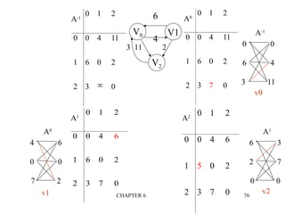
* Figure 6.33: Directed graph and its cost matrix (p.299)
V0
V2
V1
6
4
3 11 2
(a)Digraph G (b)Cost adjacency matrix for G
0 1 2
0 0 4 11
1 6 0 2
2 3  0

76. CHAPTER 6 76
0 1 2
0 0 4 11
1 6 0 2
2 3  0
A-1
0 1 2
0 0 4 11
1 6 0 2
2 3 7 0
A0
0 1 2
0 0 4 6
1 6 0 2
2 3 7 0
A1
0 1 2
0 0 4 6
1 5 0 2
2 3 7 0
A2
V0
V2
V1
6
4
3 11 2
A-1
0 0
6 4
3 11
A0
4 6
0 0
7 2
A1
6 3
2 7
0 0
v0
v1 v2

77. CHAPTER 6 77
0 1 4
3
2
















0
0
1
0
0
1
0
0
0
0
0
1
0
0
0
0
0
1
0
0
0
0
0
1
0
















1
1
1
0
0
1
1
1
0
0
1
1
1
0
0
1
1
1
0
0
1
1
1
1
0
0
1
2
3
4
0
1
2
3
4 















1
1
1
0
0
1
1
1
0
0
1
1
1
0
0
1
1
1
1
0
1
1
1
1
1
0
1
2
3
4
(a) Digraph G (b) Adjacency matrix A for G
(c) transitive closure matrix A+
(d) reflexive transitive closure matrix A*
cycle
reflexiv
e
Transitive Closure
Goal: given a graph with unweighted edges, determine if there is a path
from i to j for all i and j.
(1) Require positive path (> 0) lengths.
(2) Require nonnegative path (0) lengths.
There is a path of length > 0 There is a path of length 0
transitive closure matrix
reflexive transitive closure matrix

78. CHAPTER 6 78
Activity on Vertex (AOV) Network
definition
A directed graph in which the vertices represent
tasks or activities and the edges represent
precedence relations between tasks.
predecessor (successor)
vertex i is a predecessor of vertex j iff there is a
directed path from i to j. j is a successor of i.
partial order
a precedence relation which is both transitive (i, j,
k, ij & jk => ik ) and irreflexive (x xx).
acylic graph
a directed graph with no directed cycles

79. CHAPTER 6 79
*Figure 6.38: An AOV network (p.305)
Topological order:
linear ordering of vertices
of a graph
i, j if i is a predecessor of
j, then i precedes j in the
linear ordering
C1, C2, C4, C5, C3, C6, C8,
C7, C10, C13, C12, C14, C15,
C11, C9
C4, C5, C2, C1, C6, C3, C8,
C15, C7, C9, C10, C11, C13,
C12, C14

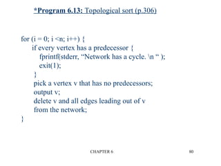
80. CHAPTER 6 80
*Program 6.13: Topological sort (p.306)
for (i = 0; i <n; i++) {
if every vertex has a predecessor {
fprintf(stderr, “Network has a cycle. n “ );
exit(1);
}
pick a vertex v that has no predecessors;
output v;
delete v and all edges leading out of v
from the network;
}

81. CHAPTER 6 81
*Figure 6.39:Simulation of Program 6.13 on an AOV
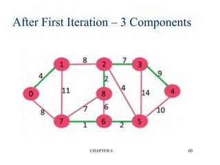
network (p.306)
v0 no predecessor
delete v0->v1, v0->v2, v0->v3
v1, v2, v3 no predecessor
select v3
delete v3->v4, v3->v5
select v2
delete v2->v4, v2->v5
select v5 select v1
delete v1->v4

82. CHAPTER 6 82
Issues in Data Structure
Consideration
Decide whether a vertex has any predecessors.
–Each vertex has a count.
Decide a vertex together with all its incident
edges.
–Adjacency list

83. CHAPTER 6 83
*Figure 6.40:Adjacency list representation of Figure 6.30(a)
(p.309)
0  1  2  3 NULL
1  4 NULL
1  4  5 NULL
1  5  4 NULL
3 NULL
2 NULL
V0
V1
V2
V3
V4
V5
v0
v1
v2
v3
v4
v5
count link
headnodes
vertex link
node

84. CHAPTER 6 84
*(p.307)
typedef struct node *node_pointer;
typedef struct node {
int vertex;
node_pointer link;
};
typedef struct {
int count;
node_pointer link;
} hdnodes;
hdnodes graph[MAX_VERTICES];

85. CHAPTER 6 85
*Program 6.14: Topological sort (p.308)
O(n)
void topsort (hdnodes graph [] , int n)
{
int i, j, k, top;
node_pointer ptr;
/* create a stack of vertices with no predecessors */
top = -1;
for (i = 0; i < n; i++)
if (!graph[i].count) {no predecessors, stack is linked through
graph[i].count = top; count field
top = i;
}
for (i = 0; i < n; i++)
if (top == -1) {
fprintf(stderr, “n Network has a cycle. Sort terminated. n”);
exit(1);
}

86. CHAPTER 6 86
O(e)
O(e+n)
Continued
}
else {
j = top; /* unstack a vertex */
top = graph[top].count;
printf(“v%d, “, j);
for (ptr = graph [j]. link; ptr ;ptr = ptr ->link ){
/* decrease the count of the successor vertices of j */
k = ptr ->vertex;
graph[k].count --;
if (!graph[k].count) {
/* add vertex k to the stack*/
graph[k].count = top;
top = k;
}
}
}
}

87. CHAPTER 6 87
Activity on Edge (AOE)
Networks
directed edge
–tasks or activities to be performed
vertex
–events which signal the completion of certain activities
number
–time required to perform the activity

88. CHAPTER 6 88
*Figure 6.41:An AOE network(p.310)
concurrent

89. CHAPTER 6 89
Application of AOE Network
Evaluate performance
–minimum amount of time
–activity whose duration time should be shortened
–…
Critical path
–a path that has the longest length
–minimum time required to complete the project
–v0, v1, v4, v7, v8 or v0, v1, v4, v6, v8 (18)

90. CHAPTER 6 90
other factors
Earliest time that vi can occur
–the length of the longest path from v0 to vi
–the earliest start time for all activities leaving vi
–early(6) = early(7) = 7
Latest time of activity
–the latest time the activity may start without increasing
the project duration
–late(5)=8, late(7)=7
Critical activity
–an activity for which early(i)=late(i)
–early(7)=late(7)
late(i)-early(i)
–measure of how critical an activity is
–late(5)-early(5)=8-5=3

91. CHAPTER 6 91
v0
v1
v2
v3
v4
v5
v6
v7
v8
a0=6
a1=4
a2=5
a3=1
a4=1
a5=2
a6=9
a7=7
a9=2
a10=4
a8=4
earliest, early, latest, late
0
0
6
6
7
7
16
16
18
0
4
4 7
14
14
0
5
5
7
7
0
0
6
6
7
7
16
10
18
2
6
6
14
14
14
10
8
8
3

92. CHAPTER 6 92
Determine Critical Paths
Delete all noncritical activities
Generate all the paths from the start to
finish vertex.

93. CHAPTER 6 93
Calculation of Earliest Times
vk vl
ai
early(i)=earliest(k)
late(i)=latest(l)-duration of ai
earliest[0]=0
earliest[j]=max{earliest[i]+duration of <i,j>}
i p(j)
earliest[j]
–the earliest event occurrence time
latest[j]
–the latest event occurrence time

94. CHAPTER 6 94
vi1
vi2
vin
.
.
.
vj
forward stage
if (earliest[k] < earliest[j]+ptr->duration)
earliest[k]=earliest[j]+ptr->duration

95. CHAPTER 6 95
*Figure 6.42:Computing earliest from topological sort
(p.313)
v0
v1
v2
v3
v4
v6
v7
v8
v5

96. CHAPTER 6 96
Calculation of Latest Times
 latest[j]
– the latest event occurrence time
latest[n-1]=earliest[n-1]
latest[j]=min{latest[i]-duration of <j,i>}
i s(j)
vi1
vi2
vin
.
.
.
vj backward stage
if (latest[k] > latest[j]-ptr->duration)
latest[k]=latest[j]-ptr->duration

97. CHAPTER 6 97
*Figure 6.43: Computing latest for AOE network of Figure 6.41(a)(p.314)

98. CHAPTER 6 98
*Figure 6.43(continued):Computing latest of AOE network of Figure 6.41(a)
(p.315)
latest[8]=earliest[8]=18
latest[6]=min{earliest[8] - 2}=16
latest[7]=min{earliest[8] - 4}=14
latest[4]=min{earliest[6] - 9;earliest[7] -7}= 7
latest[1]=min{earliest[4] - 1}=6
latest[2]=min{earliest[4] - 1}=6
latest[5]=min{earliest[7] - 4}=10
latest[3]=min{earliest[5] - 2}=8
latest[0]=min{earliest[1] - 6;earliest[2]- 4; earliest[3] -
5}=0
(c)Computation of latest from Equation (6.4) using a reverse topological
order

99. CHAPTER 6 99
*Figure 6.44:Early, late and critical values(p.316)
Activity Early Late Late-
Early
Critical
a0
a1
a2
a3
a4
a5
a6
a7
a8
a9
a10
0
0
0
6
4
5
7
7
7
16
14
0
2
3
6
6
8
7
7
10
16
14
0
2
3
0
2
3
0
0
3
0
0
Yes
No
No
Yes
No
No
Yes
Yes
No
Yes
Yes

100. CHAPTER 6 100
*Figure 6.45:Graph with noncritical activities deleted
(p.316)
V0
V4
V8
V1
V6
V7
a0
a3 a6
a7
a10
a9

101. CHAPTER 6 101
*Figure 6.46: AOE network with unreachable activities (p.317)
V0
V3
V1
V5
V2
V4
a0
a1
a2
a3
a5
a6
a4
earliest[i]=0

102. CHAPTER 6 102
*Figure 6.47: an AOE network(p.317)
V5 V8 V9
a10=5 a13=2
V2 V4 V7
a4=3 a9=4
V1 V3 V6
a2=3 a6=4
V0
a12=4
a11=2
a8=1
a7=4
a5=3
a3=6
a0=5
a1=6
start
finish