hashing

1. 1
HASH TABLES

2. Origins of the Term
 The term "hash" comes by way of
analogy with its standard meaning in
the physical world, to "chop and
mix.”
 D. Knuth notes that Hans Peter
Luhn of IBM appears to have been
the first to use the concept, in a
memo dated January 1953; the term
hash came into use some ten years
later.

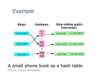
3. Concept of Hashing
 In CS, a hash table, or a hash map,
is a data structure that associates
keys (names) with values (attributes).
 Look-Up Table
 Dictionary
 Cache
 Extended Array

4. Tables of logarithms

5. Example
A small phone book as a hash table.
(Figure is from Wikipedia)

6. Just An Idea
 Hash table :
 Collection of pairs,
 Lookup function (Hash function)
 Hash tables are often used to
implement associative arrays,
 Worst-case time for Get, Insert, and
Delete is O(size).
 Expected time is O(1).

7. 7
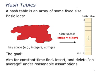
Hash Tables
A hash table is an array of some fixed size
Basic idea:
The goal:
Aim for constant-time find, insert, and delete "on
average" under reasonable assumptions
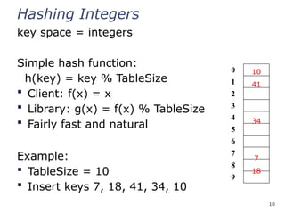
0
⁞
size -1
hash function:
index = h(key)
hash table
key space (e.g., integers, strings)

8. 8
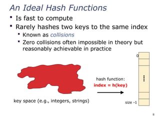
An Ideal Hash Functions
 Is fast to compute
 Rarely hashes two keys to the same index
 Known as collisions
 Zero collisions often impossible in theory but
reasonably achievable in practice
0
⁞
size -1
hash function:
index = h(key)
key space (e.g., integers, strings)

9. 9
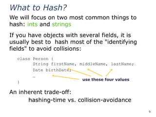
What to Hash?
We will focus on two most common things to
hash: ints and strings
If you have objects with several fields, it is
usually best to hash most of the "identifying
fields" to avoid collisions:
class Person {
String firstName, middleName, lastName;
Date birthDate;
…
}
An inherent trade-off:
hashing-time vs. collision-avoidance
use these four values

10. 10
Hashing Integers
key space = integers
Simple hash function:
h(key) = key % TableSize
 Client: f(x) = x
 Library: g(x) = f(x) % TableSize
 Fairly fast and natural
Example:
 TableSize = 10
 Insert keys 7, 18, 41, 34, 10
0
1
2
3
4
5
6
7
8
9
7
18
41
34
10

11. 11
Hashing non-integer keys
If keys are not ints, the client must provide a
means to convert the key to an int
Programming Trade-off:
 Calculation speed
 Avoiding distinct keys hashing to same ints

12. 12
Hashing Strings
Key space K = s0s1s2…sk-1
where si are chars: si  [0, 256]
Some choices: Which ones best avoid collisions?
h(K)=(s0)% TableSize
h(K)=
(∑
i=0
k −1
si)% TableSize
h(K)=
(∑
i=0
k −1
si∙37𝑖
)% TableSize

13. 13
Combining Hash Functions
A few rules of thumb / tricks:
1. Use all 32 bits (be careful with negative numbers)
2. Use different overlapping bits for different parts of the hash
 This is why a factor of 37i
works better than 256i
 Example: "abcde" and "ebcda"
3. When smashing two hashes into one hash, use bitwise-xor
 bitwise-and produces too many 0 bits
 bitwise-or produces too many 1 bits
4. Rely on expertise of others; consult books and other
resources for standard hashing functions
5. Advanced: If keys are known ahead of time, a perfect hash
can be calculated

14. 14

15. 15
COLLISION RESOLUTION
Calling a State Farm agent is not an option…

16. 16
Collision Avoidance
With (x%TableSize), number of collisions depends on
 the ints inserted
 TableSize
Larger table-size tends to help, but not always
 Example: 70, 24, 56, 43, 10
with TableSize = 10 and TableSize = 60
Technique: Pick table size to be prime. Why?
 Real-life data tends to have a pattern,
 "Multiples of 61" are probably less likely than
"multiples of 60"
 Some collision strategies do better with prime size

17. 17
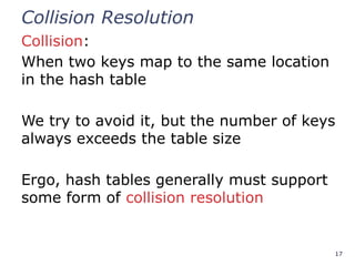
Collision Resolution
Collision:
When two keys map to the same location
in the hash table
We try to avoid it, but the number of keys
always exceeds the table size
Ergo, hash tables generally must support
some form of collision resolution

18. 18
Flavors of Collision Resolution
Separate Chaining
Open Addressing
 Linear Probing
 Quadratic Probing
 Double Hashing

19. Terminology Warning
We and the book use the terms
 "chaining" or "separate chaining"
 "open addressing"
Very confusingly, others use the terms
 "open hashing" for "chaining"
 "closed hashing" for "open addressing"
We also do trees upside-down
19

20. 20
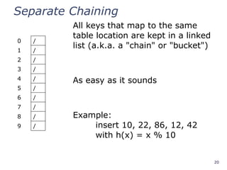
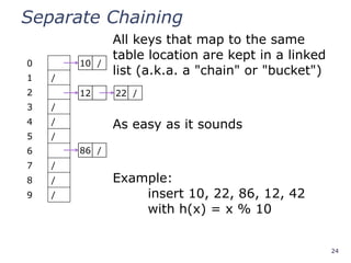
Separate Chaining
0 /
1 /
2 /
3 /
4 /
5 /
6 /
7 /
8 /
9 /
All keys that map to the same
table location are kept in a linked
list (a.k.a. a "chain" or "bucket")
As easy as it sounds
Example:
insert 10, 22, 86, 12, 42
with h(x) = x % 10

21. 21
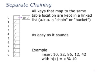
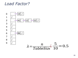
Separate Chaining
0
1 /
2 /
3 /
4 /
5 /
6 /
7 /
8 /
9 /
All keys that map to the same
table location are kept in a linked
list (a.k.a. a "chain" or "bucket")
As easy as it sounds
Example:
insert 10, 22, 86, 12, 42
with h(x) = x % 10
10 /

22. 22
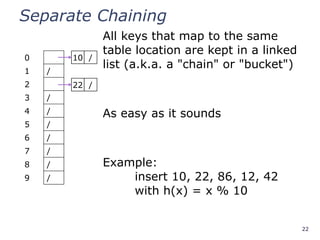
Separate Chaining
0
1 /
2
3 /
4 /
5 /
6 /
7 /
8 /
9 /
All keys that map to the same
table location are kept in a linked
list (a.k.a. a "chain" or "bucket")
As easy as it sounds
Example:
insert 10, 22, 86, 12, 42
with h(x) = x % 10
10 /
22 /

23. 23
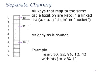
Separate Chaining
0
1 /
2
3 /
4 /
5 /
6
7 /
8 /
9 /
All keys that map to the same
table location are kept in a linked
list (a.k.a. a "chain" or "bucket")
As easy as it sounds
Example:
insert 10, 22, 86, 12, 42
with h(x) = x % 10
10 /
22 /
86 /

24. 24
Separate Chaining
0
1 /
2
3 /
4 /
5 /
6
7 /
8 /
9 /
All keys that map to the same
table location are kept in a linked
list (a.k.a. a "chain" or "bucket")
As easy as it sounds
Example:
insert 10, 22, 86, 12, 42
with h(x) = x % 10
10 /
12
86 /
22 /

25. 25
Separate Chaining
0
1 /
2
3 /
4 /
5 /
6
7 /
8 /
9 /
All keys that map to the same
table location are kept in a linked
list (a.k.a. a "chain" or "bucket")
As easy as it sounds
Example:
insert 10, 22, 86, 12, 42
with h(x) = x % 10
10 /
42
86 /
12 22 /

26. 26
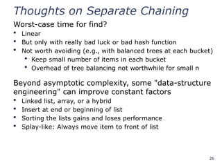
Thoughts on Separate Chaining
Worst-case time for find?
 Linear
 But only with really bad luck or bad hash function
 Not worth avoiding (e.g., with balanced trees at each bucket)
 Keep small number of items in each bucket
 Overhead of tree balancing not worthwhile for small n
Beyond asymptotic complexity, some "data-structure
engineering" can improve constant factors
 Linked list, array, or a hybrid
 Insert at end or beginning of list
 Sorting the lists gains and loses performance
 Splay-like: Always move item to front of list

27. 27
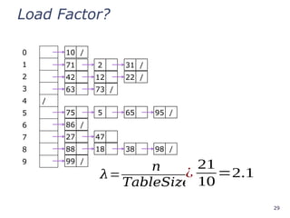
Rigorous Separate Chaining Analysis
The load factor, , of a hash table is calculated as
where n is the number of items currently in the table

28. 28
Load Factor?
0
1 /
2
3 /
4 /
5 /
6
7 /
8 /
9 /
10 /
42
86 /
12 22 /
𝜆=
𝑛
𝑇𝑎𝑏𝑙𝑒𝑆𝑖𝑧𝑒
=?
¿
5
10
=0.5

29. 29
Load Factor?
0
1
2
3
4 /
5
6
7
8
9
10 /
42
86 /
12 22 /
𝜆=
𝑛
𝑇𝑎𝑏𝑙𝑒𝑆𝑖𝑧𝑒
=?
¿
21
10
=2.1
71 2 31 /
63 73 /
75 5 65 95 /
27 47
88 18 38 98 /
99 /

30. 30

31. 31
Rigorous Separate Chaining Analysis
The load factor, , of a hash table is calculated as
where n is the number of items currently in the table
Under chaining, the average number of elements per
bucket is 
So if some inserts are followed by random finds, then
on average:
 Each unsuccessful find compares against  items
 Each successful find compares against  items
 If  is low, find and insert likely to be O(1)
 We like to keep  around 1 for separate chaining

32. 32
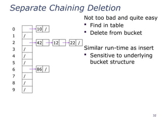
Separate Chaining Deletion
Not too bad and quite easy
 Find in table
 Delete from bucket
Similar run-time as insert
 Sensitive to underlying
bucket structure
0
1 /
2
3 /
4 /
5 /
6
7 /
8 /
9 /
10 /
42
86 /
12 22 /

33. 33
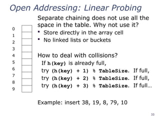
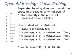
Open Addressing: Linear Probing
Separate chaining does not use all the
space in the table. Why not use it?
 Store directly in the array cell
 No linked lists or buckets
How to deal with collisions?
If h(key) is already full,
try (h(key) + 1) % TableSize. If full,
try (h(key) + 2) % TableSize. If full,
try (h(key) + 3) % TableSize. If full…
Example: insert 38, 19, 8, 79, 10
0
1
2
3
4
5
6
7
8
9

34. 34
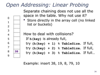
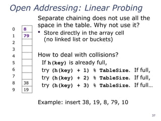
Open Addressing: Linear Probing
Separate chaining does not use all the
space in the table. Why not use it?
 Store directly in the array cell (no linked
list or buckets)
How to deal with collisions?
If h(key) is already full,
try (h(key) + 1) % TableSize. If full,
try (h(key) + 2) % TableSize. If full,
try (h(key) + 3) % TableSize. If full…
Example: insert 38, 19, 8, 79, 10
0
1
2
3
4
5
6
7
8 38
9

35. 35
Open Addressing: Linear Probing
Separate chaining does not use all the
space in the table. Why not use it?
 Store directly in the array cell
(no linked list or buckets)
How to deal with collisions?
If h(key) is already full,
try (h(key) + 1) % TableSize. If full,
try (h(key) + 2) % TableSize. If full,
try (h(key) + 3) % TableSize. If full…
Example: insert 38, 19, 8, 79, 10
0
1
2
3
4
5
6
7
8 38
9 19

36. 36
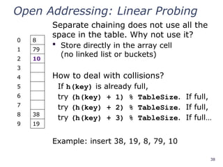
Open Addressing: Linear Probing
Separate chaining does not use all the
space in the table. Why not use it?
 Store directly in the array cell
(no linked list or buckets)
How to deal with collisions?
If h(key) is already full,
try (h(key) + 1) % TableSize. If full,
try (h(key) + 2) % TableSize. If full,
try (h(key) + 3) % TableSize. If full…
Example: insert 38, 19, 8, 79, 10
0 8
1
2
3
4
5
6
7
8 38
9 19

37. 37
Open Addressing: Linear Probing
Separate chaining does not use all the
space in the table. Why not use it?
 Store directly in the array cell
(no linked list or buckets)
How to deal with collisions?
If h(key) is already full,
try (h(key) + 1) % TableSize. If full,
try (h(key) + 2) % TableSize. If full,
try (h(key) + 3) % TableSize. If full…
Example: insert 38, 19, 8, 79, 10
0 8
1 79
2
3
4
5
6
7
8 38
9 19

38. 38
Open Addressing: Linear Probing
Separate chaining does not use all the
space in the table. Why not use it?
 Store directly in the array cell
(no linked list or buckets)
How to deal with collisions?
If h(key) is already full,
try (h(key) + 1) % TableSize. If full,
try (h(key) + 2) % TableSize. If full,
try (h(key) + 3) % TableSize. If full…
Example: insert 38, 19, 8, 79, 10
0 8
1 79
2 10
3
4
5
6
7
8 38
9 19

39. 39
Load Factor?
0 8
1 79
2 10
3
4
5
6
7
8 38
9 19
𝜆=
𝑛
𝑇𝑎𝑏𝑙𝑒𝑆𝑖𝑧𝑒
=?
¿
5
10
=0.5
Can the load factor when using
linear probing ever exceed 1.0?
Nope!!

40. 40
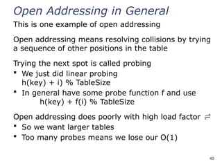
Open Addressing in General
This is one example of open addressing
Open addressing means resolving collisions by trying
a sequence of other positions in the table
Trying the next spot is called probing
 We just did linear probing
h(key) + i) % TableSize
 In general have some probe function f and use
h(key) + f(i) % TableSize
Open addressing does poorly with high load factor 
 So we want larger tables
 Too many probes means we lose our O(1)

41. 41
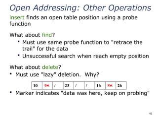
Open Addressing: Other Operations
insert finds an open table position using a probe
function
What about find?
 Must use same probe function to "retrace the
trail" for the data
 Unsuccessful search when reach empty position
What about delete?
 Must use "lazy" deletion. Why?
 Marker indicates "data was here, keep on probing"
10  / 23 / / 16  26

42. 42
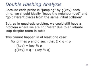
Primary Clustering
It turns out linear probing is a bad idea, even
though the probe function is quick to compute
(which is a good thing)
 This tends to produce
clusters, which lead to
long probe sequences
 This is called primary
clustering
 We saw the start of a
cluster in our linear
probing example
[R. Sedgewick]

43. 43
Analysis of Linear Probing
Trivial fact:
For any  < 1, linear probing will find an empty slot
 We are safe from an infinite loop unless table is full
Non-trivial facts (we won’t prove these):
Average # of probes given load factor 
 For an unsuccessful search as :
 For an successful search as :

44. 44
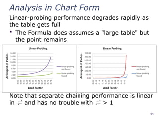
Analysis in Chart Form
Linear-probing performance degrades rapidly as
the table gets full
 The Formula does assumes a "large table" but
the point remains
Note that separate chaining performance is linear
in  and has no trouble with  > 1

45. 45
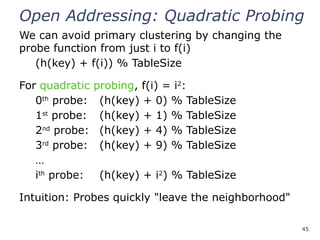
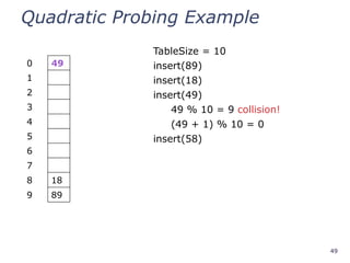
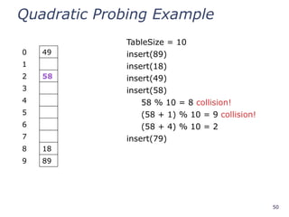
Open Addressing: Quadratic Probing
We can avoid primary clustering by changing the
probe function from just i to f(i)
(h(key) + f(i)) % TableSize
For quadratic probing, f(i) = i2
:
0th
probe: (h(key) + 0) % TableSize
1st
probe: (h(key) + 1) % TableSize
2nd
probe: (h(key) + 4) % TableSize
3rd
probe: (h(key) + 9) % TableSize
…
ith
probe: (h(key) + i2
) % TableSize
Intuition: Probes quickly "leave the neighborhood"

46. 46
Quadratic Probing Example
0
1
2
3
4
5
6
7
8
9
TableSize = 10
insert(89)

47. 47
Quadratic Probing Example
0
1
2
3
4
5
6
7
8
9 89
TableSize = 10
insert(89)
insert(18)

48. 48
Quadratic Probing Example
TableSize = 10
insert(89)
insert(18)
insert(49)
0
1
2
3
4
5
6
7
8 18
9 89

49. 49
Quadratic Probing Example
TableSize = 10
insert(89)
insert(18)
insert(49)
49 % 10 = 9 collision!
(49 + 1) % 10 = 0
insert(58)
0 49
1
2
3
4
5
6
7
8 18
9 89

50. 50
Quadratic Probing Example
TableSize = 10
insert(89)
insert(18)
insert(49)
insert(58)
58 % 10 = 8 collision!
(58 + 1) % 10 = 9 collision!
(58 + 4) % 10 = 2
insert(79)
0 49
1
2 58
3
4
5
6
7
8 18
9 89

51. 51
Quadratic Probing Example
TableSize = 10
insert(89)
insert(18)
insert(49)
insert(58)
insert(79)
79 % 10 = 9 collision!
(79 + 1) % 10 = 0 collision!
(79 + 4) % 10 = 3
0 49
1
2 58
3 79
4
5
6
7
8 18
9 89

52. 52
Another Quadratic Probing Example
0
1
2
3
4
5
6
TableSize = 7
Insert:
76 (76 % 7 = 6)
40 (40 % 7 = 5)
48 (48 % 7 = 6)
5 (5 % 7 = 5)
55 (55 % 7 = 6)
47 (47 % 7 = 5)

53. 53
Another Quadratic Probing Example
0
1
2
3
4
5
6 76
TableSize = 7
Insert:
76 (76 % 7 = 6)
40 (40 % 7 = 5)
48 (48 % 7 = 6)
5 (5 % 7 = 5)
55 (55 % 7 = 6)
47 (47 % 7 = 5)

54. 54
Another Quadratic Probing Example
0
1
2
3
4
5 40
6 76
TableSize = 7
Insert:
76 (76 % 7 = 6)
40 (40 % 7 = 5)
48 (48 % 7 = 6)
5 (5 % 7 = 5)
55 (55 % 7 = 6)
47 (47 % 7 = 5)

55. 55
Another Quadratic Probing Example
0 48
1
2
3
4
5 40
6 76
TableSize = 7
Insert:
76 (76 % 7 = 6)
40 (40 % 7 = 5)
48 (48 % 7 = 6)
5 (5 % 7 = 5)
55 (55 % 7 = 6)
47 (47 % 7 = 5)

56. 56
Another Quadratic Probing Example
0 48
1
2 5
3
4
5 40
6 76
TableSize = 7
Insert:
76 (76 % 7 = 6)
77 (40 % 7 = 5)
48 (48 % 7 = 6)
5 (5 % 7 = 5)
55 (55 % 7 = 6)
47 (47 % 7 = 5)

57. 57
Another Quadratic Probing Example
0 48
1
2 5
3 55
4
5 40
6 76
TableSize = 7
Insert:
76 (76 % 7 = 6)
40 (40 % 7 = 5)
48 (48 % 7 = 6)
5 (5 % 7 = 5)
55 (55 % 7 = 6)
47 (47 % 7 = 5)

58. 58
Another Quadratic Probing Example
0 48
1
2 5
3 55
4
5 40
6 76
TableSize = 7
Insert:
76 (76 % 7 = 6)
40 (40 % 7 = 5)
48 (48 % 7 = 6)
5 (5 % 7 = 5)
55 (55 % 7 = 6)
47 (47 % 7 = 5)
(47 + 1) % 7 = 6 collision!
(47 + 4) % 7 = 2 collision!
(47 + 9) % 7 = 0 collision!
(47 + 16) % 7 = 0 collision!
(47 + 25) % 7 = 2 collision!
Will we ever get
a 1 or 4?!?

59. 59
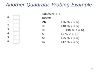
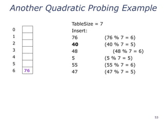
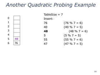
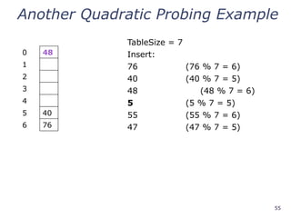
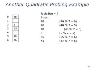
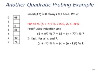
Another Quadratic Probing Example
0 48
1
2 5
3 55
4
5 40
6 76
insert(47) will always fail here. Why?
For all n, (5 + n2
) % 7 is 0, 2, 5, or 6
Proof uses induction and
(5 + n2
) % 7 = (5 + (n - 7)2
) % 7
In fact, for all c and k,
(c + n2
) % k = (c + (n - k)2
) % k

60. 60
From Bad News to Good News
After TableSize quadratic probes, we cycle
through the same indices
The good news:
 For prime T and 0  i, j  T/2 where i  j,
(h(key) + i2
) % T  (h(key) + j2
) % T
 If TableSize is prime and  < ½, quadratic
probing will find an empty slot in at most
TableSize/2 probes
 If you keep  < ½, no need to detect cycles as
we just saw

61. 61
Clustering Reconsidered
Quadratic probing does not suffer from primary
clustering as the quadratic nature quickly escapes
the neighborhood
But it is no help if keys initially hash the same index
 Any 2 keys that hash to the same value will have
the same series of moves after that
 Called secondary clustering
We can avoid secondary clustering with a probe
function that depends on the key: double hashing

62. 62
Open Addressing: Double Hashing
Idea:
Given two good hash functions h and g, it is very
unlikely that for some key, h(key) == g(key)
Ergo, why not probe using g(key)?
For double hashing, f(i) = i ⋅ g(key):
0th
probe: (h(key) + 0 ⋅ g(key)) % TableSize
1st
probe: (h(key) + 1 ⋅ g(key)) % TableSize
2nd
probe: (h(key) + 2 ⋅ g(key)) % TableSize
…
ith
probe: (h(key) + i ⋅ g(key)) % TableSize
Crucial Detail:
We must make sure that g(key) cannot be 0

63. 63
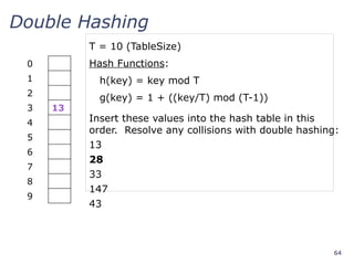
Double Hashing
Insert these values into the hash table in this
order. Resolve any collisions with double hashing:
13
28
33
147
43
T = 10 (TableSize)
Hash Functions:
h(key) = key mod T
g(key) = 1 + ((key/T) mod (T-1))
0
1
2
3
4
5
6
7
8
9

64. 64
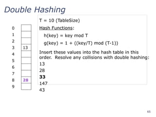
Double Hashing
Insert these values into the hash table in this
order. Resolve any collisions with double hashing:
13
28
33
147
43
T = 10 (TableSize)
Hash Functions:
h(key) = key mod T
g(key) = 1 + ((key/T) mod (T-1))
0
1
2
3 13
4
5
6
7
8
9

65. 65
Double Hashing
Insert these values into the hash table in this
order. Resolve any collisions with double hashing:
13
28
33
147
43
T = 10 (TableSize)
Hash Functions:
h(key) = key mod T
g(key) = 1 + ((key/T) mod (T-1))
0
1
2
3 13
4
5
6
7
8 28
9

66. 66
Double Hashing
Insert these values into the hash table in this
order. Resolve any collisions with double hashing:
13
28
33  g(33) = 1 + 3 mod 9 = 4
147
43
T = 10 (TableSize)
Hash Functions:
h(key) = key mod T
g(key) = 1 + ((key/T) mod (T-1))
0
1
2
3 13
4
5
6
7 33
8 28
9

67. 67
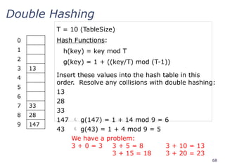
Double Hashing
Insert these values into the hash table in this
order. Resolve any collisions with double hashing:
13
28
33
147  g(147) = 1 + 14 mod 9 = 6
43
T = 10 (TableSize)
Hash Functions:
h(key) = key mod T
g(key) = 1 + ((key/T) mod (T-1))
0
1
2
3 13
4
5
6
7 33
8 28
9 147

68. 68
Double Hashing
Insert these values into the hash table in this
order. Resolve any collisions with double hashing:
13
28
33
147  g(147) = 1 + 14 mod 9 = 6
43  g(43) = 1 + 4 mod 9 = 5
T = 10 (TableSize)
Hash Functions:
h(key) = key mod T
g(key) = 1 + ((key/T) mod (T-1))
0
1
2
3 13
4
5
6
7 33
8 28
9 147
We have a problem:
3 + 0 = 3 3 + 5 = 8 3 + 10 = 13
3 + 15 = 18 3 + 20 = 23

69. 69
Double Hashing Analysis
Because each probe is "jumping" by g(key) each
time, we should ideally "leave the neighborhood" and
"go different places from the same initial collision"
But, as in quadratic probing, we could still have a
problem where we are not "safe" due to an infinite
loop despite room in table
This cannot happen in at least one case:
For primes p and q such that 2 < q < p
h(key) = key % p
g(key) = q – (key % q)

70. 70
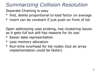
Summarizing Collision Resolution
Separate Chaining is easy
 find, delete proportional to load factor on average
 insert can be constant if just push on front of list
Open addressing uses probing, has clustering issues
as it gets full but still has reasons for its use:
 Easier data representation
 Less memory allocation
 Run-time overhead for list nodes (but an array
implementation could be faster)

71. 71
REHASHING
When you make hash from hash leftovers…

72. 72
Rehashing
As with array-based stacks/queues/lists
 If table gets too full, create a bigger table and copy
everything
 Less helpful to shrink a table that is underfull
With chaining, we get to decide what "too full" means
 Keep load factor reasonable (e.g., < 1)?
 Consider average or max size of non-empty chains
For open addressing, half-full is a good rule of thumb

73. 73
Rehashing
What size should we choose?
 Twice-as-big?
 Except that won’t be prime!
We go twice-as-big but guarantee prime
 Implement by hard coding a list of prime numbers
 You probably will not grow more than 20-30 times
and can then calculate after that if necessary

74. 74
Rehashing
Can we copy all data to the same indices in the new table?
 Will not work; we calculated the index based on TableSize
Rehash Algorithm:
Go through old table
Do standard insert for each item into new table
Resize is an O(n) operation,
 Iterate over old table: O(n)
 n inserts / calls to the hash function: n ⋅ O(1) = O(n)
Is there some way to avoid all those hash function calls?
 Space/time tradeoff: Could store h(key) with each data item
 Growing the table is still O(n); only helps by a constant
factor

75. 75
IMPLEMENTING HASHING
Reality is never as clean-cut as theory

76. 76
Hashing and Comparing
Our use of int key can lead to us overlooking a
critical detail
 We do perform the initial hash on E
 While chaining/probing, we compare to E which requires
equality testing (compare == 0)
A hash table needs a hash function and a comparator
 In Project 2, you will use two function objects
 The Java library uses a more object-oriented approach:
each object has an equals method and a hashCode
method:
class Object {
boolean equals(Object o) {…}
int hashCode() {…}
…
}

77. 77
Equal Objects Must Hash the Same
The Java library (and your project hash table) make
a very important assumption that clients must satisfy
Object-oriented way of saying it:
If a.equals(b), then we must require
a.hashCode()==b.hashCode()
Function object way of saying it:
If c.compare(a,b) == 0, then we must require
h.hash(a) == h.hash(b)
If you ever override equals
 You need to override hashCode also in a consistent way
 See CoreJava book, Chapter 5 for other "gotchas" with
equals

78. 78
Comparable/Comparator Rules
We have not emphasized important "rules"
about comparison for:
 all our dictionaries
 sorting (next major topic)
Comparison must impose a consistent,
total ordering:
For all a, b, and c:
 If compare(a,b) < 0, then compare(b,a) > 0
 If compare(a,b) == 0, then compare(b,a) == 0
 If compare(a,b) < 0 and compare(b,c) < 0,
then compare(a,c) < 0

79. 79
A Generally Good hashCode()
int result = 17; // start at a prime
foreach field f
int fieldHashcode =
boolean: (f ? 1: 0)
byte, char, short, int: (int) f
long: (int) (f ^ (f >>> 32))
float: Float.floatToIntBits(f)
double: Double.doubleToLongBits(f), then above
Object: object.hashCode( )
result = 31 * result + fieldHashcode;
return result;

80. 80
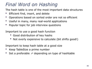
Final Word on Hashing
The hash table is one of the most important data structures
 Efficient find, insert, and delete
 Operations based on sorted order are not so efficient
 Useful in many, many real-world applications
 Popular topic for job interview questions
Important to use a good hash function
 Good distribution of key hashs
 Not overly expensive to calculate (bit shifts good!)
Important to keep hash table at a good size
 Keep TableSize a prime number
 Set a preferable  depending on type of hashtable

81. 81
MIDTERM EXAM
Are you ready… for an exam?

82. 82
The Midterm
It is next Wednesday, July 18
It will take up the entire class period
It will cover everything up through today:
 Algorithmic analysis, Big-O, Recurrences
 Heaps and Priority Queues
 Stacks, Queues, Arrays, Linked Lists, etc.
 Dictionaries
 Regular BSTs, Balanced Trees, and B-Trees
 Hash Tables

83. 83
The Midterm
The exam consists of 10 problems
 Total points possible is 110
 Your score will be out of 100
 Yes, you could score as well as 110/100
Types of Questions:
 Some calculations
 Drill problems manipulating data structures
 Writing pseudocode solutions

84. 84
Book, Calculator, and Notes
The exam is closed book
You can bring a calculator if you want
You can bring a limited set of notes:
 One 3x5 index card (both sides)
 Must be handwritten (no typing!)
 You must turn in the card with your exam

85. 85
Preparing for the Exam
Quiz section tomorrow is a review
 Come with questions for David
We might do an exam review session
 Only if you show interest
Previous exams available for review
 Look for the link on midterm information

86. 86
Kate's General Exam Advice
Get a good night's sleep
Eat some breakfast
Read through the exam before you start
Write down partial work
Remember the class is curved at the end

87. 87
PRACTICE PROBLEMS

88. 88
Improving Linked Lists
For reasons beyond your control, you have
to work with a very large linked list. You
will be doing many finds, inserts, and
deletes. Although you cannot stop using a
linked list, you are allowed to modify the
linked structure to improve performance.
What can you do?

89. 89
Depth Traversal of a Tree
One way to list the nodes of a BST is the
depth traversal:
 List the root
 List the root's two children
 List the root's children's children, etc.
How would you implement this traversal?
How would you handle null children?
What is the big-O of your solution?

90. 90
Nth smallest element in a B Tree
For a B Tree, you want to implement a
function FindSmallestKey(i) which returns
the ith
smallest key in the tree.
Describe a pseudocode solution.
What is the run-time of your code?
Is it dependent on L, M, and/or n?

91. 91
Hashing a Checkerboad
One way to speed up Game AIs is to hash
and store common game states. In the case
of checkers, how would you store the game
state of:
 The 8x8 board
 The 12 red pieces (single men or kings)
 The 12 black pieces (single men or kings)
Can your solution generalize to more complex
games like chess?