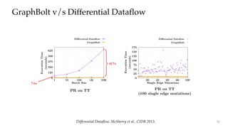
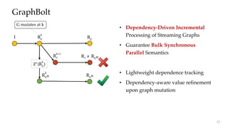
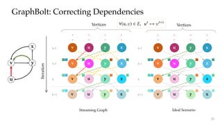
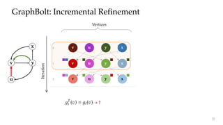
The document discusses GraphBolt, a dependency-driven system for synchronous processing of streaming graphs that guarantees bulk synchronous parallel semantics and employs lightweight dependence tracking. It highlights the challenges of managing value dependencies during graph mutations and introduces a method for incrementally correcting and tracking aggregated values rather than individual dependencies to improve efficiency. The document references various graph processing algorithms to showcase the framework's capabilities in real-time processing and low-latency computations.

1. GraphBolt: Dependency-Driven
Synchronous Processing of Streaming Graphs
Mugilan Mariappan and Keval Vora
Simon Fraser University
EuroSys’19 – Dresden, Germany
March 27, 2019

2. Graph Processing
2

3. Dynamic Graph Processing
Real-time Processing
• Low Latency
Real-time Batch Processing
• High Throughput
Alipay payments unit of Chinese retailer Alibaba [..]
has 120 billion nodes and over 1 trillion relationships [..];
this graph has 2 billion updates each day and was running
at 250,000 transactions per second on Singles Day [..]
The Graph Database Poised to Pounce on The Mainstream. Timothy Prickett Morgan, The Next Platform. September 19, 2018. 3

4. KickStarter [ASPLOS’17]
KickStarter: Fast and Accurate Computations on Streaming Graph via Trimmed Approximations. Vora et al., ASPLOS 2017.
... ...
Query
Graph
Mutations
Incremental Processing
• Adjust results incrementally
• Reuse work that has already been done
Tornado [SIGMOD’16]
GraphIn [EuroPar’16]
KineoGraph [EuroSys’12]
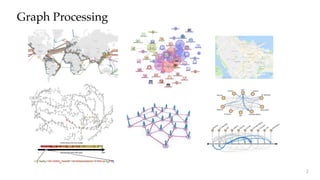
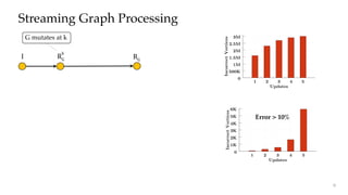
Streaming Graph Processing
Tag Propagation
upon mutation
Over 75% values get thrown out
4

5. KickStarter: Fast and Accurate Computations on Streaming Graph via Trimmed Approximations. Vora et al., ASPLOS 2017.
... ...
Query
Graph
Mutations
Incremental Processing
• Adjust results incrementally
• Reuse work that has already been done
Tornado [SIGMOD’16]
GraphIn [EuroPar’16]
KineoGraph [EuroSys’12]
KickStarter [ASPLOS’17]
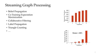
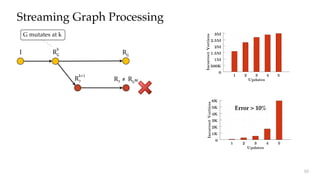
Streaming Graph Processing
Maintain Value Dependences
Incrementally refine results
Less than 0.0005% values thrown out
5

6. KickStarter: Fast and Accurate Computations on Streaming Graph via Trimmed Approximations. Vora et al., ASPLOS 2017.
... ...
Query
Graph
Mutations
Incremental Processing
• Adjust results incrementally
• Reuse work that has already been done
Tornado [SIGMOD’16]
GraphIn [EuroPar’16]
KineoGraph [EuroSys’12]
KickStarter [ASPLOS’17]
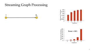
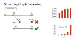
Streaming Graph Processing
Maintain Value Dependences
Incrementally refine results
Less than 0.0005% values thrown out
Monotonic Graph
Algorithms
6

7. Streaming Graph Processing
• Belief Propagation
• Co-Training Expectation
Maximization
• Collaborative Filtering
• Label Propagation
• Triangle Counting
• …
0
500K
1M
1.5M
2M
2.5M
3M
1 2 3 4 5
IncorrectVertices
Updates
0
1K
2K
3K
4K
5K
6K
1 2 3 4 5
IncorrectVertices
Updates
Error > 10%
7

8. Streaming Graph Processing
0
500K
1M
1.5M
2M
2.5M
3M
1 2 3 4 5
IncorrectVertices
Updates
0
1K
2K
3K
4K
5K
6K
1 2 3 4 5
IncorrectVertices
Updates
Error > 10%
I RG
8

9. Streaming Graph Processing
0
500K
1M
1.5M
2M
2.5M
3M
1 2 3 4 5
IncorrectVertices
Updates
0
1K
2K
3K
4K
5K
6K
1 2 3 4 5
IncorrectVertices
Updates
Error > 10%
I RG
k
RG
G mutates at k
9

10. Streaming Graph Processing
0
500K
1M
1.5M
2M
2.5M
3M
1 2 3 4 5
IncorrectVertices
Updates
0
1K
2K
3K
4K
5K
6K
1 2 3 4 5
IncorrectVertices
Updates
Error > 10%
I RG
k
RG
R?
k+1
G mutates at k
R? ≠ RGM
10

11. Streaming Graph Processing
0
500K
1M
1.5M
2M
2.5M
3M
1 2 3 4 5
IncorrectVertices
Updates
0
1K
2K
3K
4K
5K
6K
1 2 3 4 5
IncorrectVertices
Updates
Error > 10%
I RG
k
RG
R?
k+1
R? ≠ RGM
R
k
GM RGM
Zs
(RG
k
)
G mutates at k
11

12. GraphBolt
I RG
k
RG
R?
k+1
R? ≠ RGM
R
k
GM RGM
Zs
(RG
k
)
G mutates at k
• Dependency-Driven Incremental
Processing of Streaming Graphs
• Guarantee Bulk Synchronous
Parallel Semantics
• Lightweight dependence tracking
• Dependency-aware value refinement
upon graph mutation
12

13. v u y xk-1
u
yv
x
Iteration
Vertices
Bulk Synchronous Processing (BSP)
v u y xk
Streaming Graph
13

14. v u y x
v u y x
Upon Edge Addition
k-1
ku
yv
x
Iteration
Vertices
Streaming Graph
14

15. v u y x
v u y x
v u y x
Upon Edge Addition
k-1
k
k+1
u
yv
x
Iteration
Vertices
Streaming Graph
15

16. v u y x
v u y x
v u y x
Upon Edge Addition
k-1
ku
yv
x
Iteration
Vertices
Streaming Graph
v u y x
v u y x
v u y x
Ideal Scenario
k-1
k
Vertices
16

17. v u y x
v u y x
v u y x
Upon Edge Addition
k-1
ku
yv
x
Iteration
Vertices
Streaming Graph
v u y x
v u y x
v u y x
Ideal Scenario
k-1
k
Vertices
17

18. v u y x
v u y x
v u y x
Upon Edge Addition
k-1
k
k+1
u
yv
x
Iteration
Vertices
Streaming Graph
v u y x
v u y x
v u y x
Ideal Scenario
k-1
k
k+1
Vertices
18

19. yk v u
v u y
v u y
v u y
v u y
v u y
v u y
v u y
Upon Edge Addition
k-1
k+1
k-2
u
yv
x
Iteration
k-1
k
k+1
k-2
Vertices Vertices
x
x
x
x
x
x
x
x
Ideal ScenarioStreaming Graph
19

20. yk v u
v u y
v u y
v u y
v u y
v u y
v u y
v u y
Upon Edge Addition
k-1
k+1
k-2
u
yv
x
Iteration
k-1
k
k+1
k-2
Vertices Vertices
x
x
x
x
x
x
x
x
Ideal ScenarioStreaming Graph
20

21. yk v u
v u y
v u y
v u y
v u y
v u y
v u y
Upon Edge Addition
k-1
k+1
k-2
u
yv
x
Iteration
k-1
k
k+1
k-2
Vertices Vertices
x
x
x
x
x
x
x
Ideal ScenarioStreaming Graph
yv u y x
21

22. yk v u
v u y
v u y
v u y
v u y
v u y
v u y
v u y
Upon Edge Addition
k-1
k+1
k-2
u
yv
x
Iteration
k-1
k
k+1
k-2
Vertices Vertices
x
x
x
x
x
x
x
x
Ideal ScenarioStreaming Graph
22

23. y
vv
vv
u x x
y
Upon Edge Deletion
u
yv
x
Iteration
u y
u y
v y
v u
v u y
v u y
v u y
v u y
Ideal Scenario
k-1
k
k+1
k-2
Iteration
k-1
k
k+1
k-2
Vertices Vertices
x
x
x
x
x
x
y
u x
Streaming Graph
23

24. v u y
v u y
v u y
v u y
v u y
v u y
Ideal Scenario
k-1
k
k-2
u
yv
x
Iteration
k-1
k
k-2
Vertices Vertices
x
x
x
x
x
x
GraphBolt: Correcting Dependencies
Streaming Graph
24

25. v u y x
v u y x
v u y x
v u y
v u y
v u y
Ideal Scenario
k-1
k
k-2
u
yv
x
Iteration
k-1
k
k-2
Vertices Vertices
x
x
x
GraphBolt: Correcting Dependencies
Streaming Graph
25

26. xv u y
v u y x
v u y x v u y
v u y
v u y
Ideal Scenario
k-1
k
k-2
u
yv
x
Iteration
k-1
k
k-2
Vertices Vertices
x
x
x
GraphBolt: Correcting Dependencies
Streaming Graph
26

27. xv u y
v u y x
v u y x v u y
v u y
v u y
Ideal Scenario
k-1
k
k-2
u
yv
x
Iteration
k-1
k
k-2
Vertices Vertices
x
x
x
GraphBolt: Correcting Dependencies
Streaming Graph
27

28. xv u y
v u y x
v u y xxv u y v u y
v u y
v u y
Ideal Scenario
k-1
k
k-2
u
yv
x
Iteration
k-1
k
k-2
Vertices Vertices
x
x
x
GraphBolt: Correcting Dependencies
Streaming Graph
28

29. xv u y
v u y x
v u y xxv u y v u y
v u y
v u y
Ideal Scenario
k-1
k
k-2
u
yv
x
Iteration
k-1
k
k-2
Vertices Vertices
x
x
x
GraphBolt: Correcting Dependencies
Streaming Graph
k+1k+1 v u y xv u y x
29

30. u y
v
GraphBolt: Dependency Tracking
vk
u xk-1
Iteration
ofCL for subsequent graph mutations, such tracking of value
dependencies leads to O |E|.t amount of information to be
maintained for t iterations which signicantly increases the
memory footprint, making the entire process memory-bound.
To reduce the amount of dependency information that must
be tracked, we rst carefully analyze how values owing
through dependencies participate in computing CL.
Tracking Value Dependencies as Value Aggregations.
Given a vertex , its value is computed based on values from
its incoming neighbors in two sub-steps: rst, the incoming
neighbors’ values from previous iteration are aggregated into
a single value; and then, the aggregated value is used to com-
pute vertex value for the current iteration. This computation
can be formulated as 2:
ci ( ) =
º
(
8e=(u, )2E
(ci 1(u)) )
where
…
indicates the aggregation operator and
≤
indicates
the function applied on the aggregated value to produce the
nal vertex value. For example in Algorithm 1,
…
is
A on line 6 while
≤
is the computation on line 9. Since
values owing through edges are eectively combined into
input graph (see Eq. 1), i.e.,
Figure 2a. Since we are no l
through those dependency
dependency structure as it
the renement stage using
we only need to track agg
reduces the amount of dep
Pruning Value Aggregat
The skewed nature of rea
synchronous graph algori
vertex values keep on chan
and then the number of ch
ations progress. For exam
values change across itera
Wiki graph (graph details
dow. As we can see, the col
iterations indicating that m
those iterations; after 5 iter
the color density decreases
corresponding aggregated v
a useful opportunity to limi
that must be tracked durin
We conservatively prun
a single value; and then, the aggregated value is used to com-
pute vertex value for the current iteration. This computation
can be formulated as 2:
ci ( ) =
º
(
8e=(u, )2E
(ci 1(u)) )
where
…
indicates the aggregation operator and
≤
indicates
the function applied on the aggregated value to produce the
nal vertex value. For example in Algorithm 1,
…
is
A on line 6 while
≤
is the computation on line 9. Since
values owing through edges are eectively combined into
aggregated values at vertices, we can track these aggregated
values instead of individual dependency information. By
doing so, value dependencies can be corrected upon graph
mutation by incrementally correcting the aggregated values
and propagating corrections across subsequent aggregations
throughout the graph.
Let i ( ) be the aggregated value for vertex for iteration
i, i.e., i ( ) =
…
8e=(u, )2E
(ci 1(u)). We dene AG = (VA, EA) as
dependency graph in terms of aggregation values at the end
of iteration k:
– EA = { ( i 1(u), i ( )) :
and then the num
ations progress.
values change ac
Wiki graph (grap
dow. As we can s
iterations indicat
those iterations; a
the color density
corresponding ag
a useful opportun
that must be trac
We conservati
balance the mem
values with recom
particular, we in
pruning over the
dierent dimens
tal pruning is ac
of aggregated va
the horizontal re
which aggregated
on the other hand
by not saving ag
v = ( )
memory footprint, making the entire process memory-bound.
To reduce the amount of dependency information that must
be tracked, we rst carefully analyze how values owing
through dependencies participate in computing CL.
Tracking Value Dependencies as Value Aggregations.
Given a vertex , its value is computed based on values from
its incoming neighbors in two sub-steps: rst, the incoming
neighbors’ values from previous iteration are aggregated into
a single value; and then, the aggregated value is used to com-
pute vertex value for the current iteration. This computation
can be formulated as 2:
ci ( ) =
º
(
8e=(u, )2E
(ci 1(u)) )
where
…
indicates the aggregation operator and
≤
indicates
the function applied on the aggregated value to produce the
nal vertex value. For example in Algorithm 1,
…
is
A on line 6 while
≤
is the computation on line 9. Since
values owing through edges are eectively combined into
aggregated values at vertices, we can track these aggregated
values instead of individual dependency information. By
doing so, value dependencies can be corrected upon graph
dependency structure as it c
the renement stage using t
we only need to track aggr
reduces the amount of depe
Pruning Value Aggregati
The skewed nature of real-
synchronous graph algorit
vertex values keep on chang
and then the number of cha
ations progress. For examp
values change across iterat
Wiki graph (graph details in
dow. As we can see, the colo
iterations indicating that ma
those iterations; after 5 itera
the color density decreases s
corresponding aggregated va
a useful opportunity to limit
that must be tracked during
We conservatively prune
balance the memory requir
values with recomputation
particular, we incorporate
30

31. u y
v
GraphBolt: Dependency Tracking
vk
u xk-1
Iteration
ofCL for subsequent graph mutations, such tracking of value
dependencies leads to O |E|.t amount of information to be
maintained for t iterations which signicantly increases the
memory footprint, making the entire process memory-bound.
To reduce the amount of dependency information that must
be tracked, we rst carefully analyze how values owing
through dependencies participate in computing CL.
Tracking Value Dependencies as Value Aggregations.
Given a vertex , its value is computed based on values from
its incoming neighbors in two sub-steps: rst, the incoming
neighbors’ values from previous iteration are aggregated into
a single value; and then, the aggregated value is used to com-
pute vertex value for the current iteration. This computation
can be formulated as 2:
ci ( ) =
º
(
8e=(u, )2E
(ci 1(u)) )
where
…
indicates the aggregation operator and
≤
indicates
the function applied on the aggregated value to produce the
nal vertex value. For example in Algorithm 1,
…
is
A on line 6 while
≤
is the computation on line 9. Since
values owing through edges are eectively combined into
input graph (see Eq. 1), i.e.,
Figure 2a. Since we are no l
through those dependency
dependency structure as it
the renement stage using
we only need to track agg
reduces the amount of dep
Pruning Value Aggregat
The skewed nature of rea
synchronous graph algori
vertex values keep on chan
and then the number of ch
ations progress. For exam
values change across itera
Wiki graph (graph details
dow. As we can see, the col
iterations indicating that m
those iterations; after 5 iter
the color density decreases
corresponding aggregated v
a useful opportunity to limi
that must be tracked durin
We conservatively prun
a single value; and then, the aggregated value is used to com-
pute vertex value for the current iteration. This computation
can be formulated as 2:
ci ( ) =
º
(
8e=(u, )2E
(ci 1(u)) )
where
…
indicates the aggregation operator and
≤
indicates
the function applied on the aggregated value to produce the
nal vertex value. For example in Algorithm 1,
…
is
A on line 6 while
≤
is the computation on line 9. Since
values owing through edges are eectively combined into
aggregated values at vertices, we can track these aggregated
values instead of individual dependency information. By
doing so, value dependencies can be corrected upon graph
mutation by incrementally correcting the aggregated values
and propagating corrections across subsequent aggregations
throughout the graph.
Let i ( ) be the aggregated value for vertex for iteration
i, i.e., i ( ) =
…
8e=(u, )2E
(ci 1(u)). We dene AG = (VA, EA) as
dependency graph in terms of aggregation values at the end
of iteration k:
– EA = { ( i 1(u), i ( )) :
and then the num
ations progress.
values change ac
Wiki graph (grap
dow. As we can s
iterations indicat
those iterations; a
the color density
corresponding ag
a useful opportun
that must be trac
We conservati
balance the mem
values with recom
particular, we in
pruning over the
dierent dimens
tal pruning is ac
of aggregated va
the horizontal re
which aggregated
on the other hand
by not saving ag
• Dependency relations translate
across aggregation points
• Structure of dependencies
inferred from input graphs
v = ( )
memory footprint, making the entire process memory-bound.
To reduce the amount of dependency information that must
be tracked, we rst carefully analyze how values owing
through dependencies participate in computing CL.
Tracking Value Dependencies as Value Aggregations.
Given a vertex , its value is computed based on values from
its incoming neighbors in two sub-steps: rst, the incoming
neighbors’ values from previous iteration are aggregated into
a single value; and then, the aggregated value is used to com-
pute vertex value for the current iteration. This computation
can be formulated as 2:
ci ( ) =
º
(
8e=(u, )2E
(ci 1(u)) )
where
…
indicates the aggregation operator and
≤
indicates
the function applied on the aggregated value to produce the
nal vertex value. For example in Algorithm 1,
…
is
A on line 6 while
≤
is the computation on line 9. Since
values owing through edges are eectively combined into
aggregated values at vertices, we can track these aggregated
values instead of individual dependency information. By
doing so, value dependencies can be corrected upon graph
dependency structure as it c
the renement stage using t
we only need to track aggr
reduces the amount of depe
Pruning Value Aggregati
The skewed nature of real-
synchronous graph algorit
vertex values keep on chang
and then the number of cha
ations progress. For examp
values change across iterat
Wiki graph (graph details in
dow. As we can see, the colo
iterations indicating that ma
those iterations; after 5 itera
the color density decreases s
corresponding aggregated va
a useful opportunity to limit
that must be tracked during
We conservatively prune
balance the memory requir
values with recomputation
particular, we incorporate
31

32. GraphBolt: Incremental Refinement
v u y
v u y
v u y
1
2
0
u
yv
x
Iteration
Vertices
x
x
x
lues upon graph mutation.
performed (e.g., dropping
d require backpropagation
ring renement to recom-
cremental computation.
Renement
es to be added to G and
ransform it to GT . Hence,
update i ( ) =
…
8e=(u, )2E
(ci 1(u)) to T
i ( ) =
…
8e=(u, )2ET
(cT
i 1(u)) for
0  i  L. This is incrementally achieved as:
T
i ( ) = i ( )
⁄
8e=(u, )2Ea
(cT
i 1(u))
ÿ
–
8e=(u, )2Ed
(ci 1(u))
ÿ
4
8e=(u, )2ET
s.t .ci 1(u),cT
i 1(u)
(cT
i 1(u))
where
“
,
–
- and
–
4 are incremental aggregation operators
+ ?
32

33. Edge additions
recomputed to be able to rene values upon graph mutation.
While aggressive pruning can be performed (e.g., dropping
certain vertices altogether), it would require backpropagation
from values that get changed during renement to recom-
pute the correct old values for incremental computation.
3.3 Dependency-Driven Value Renement
Let Ea and Ed be the set of edges to be added to G and
deleted from G respectively to transform it to GT . Hence,
GT = G [ Ea Ed . Given Ea, Ed and the dependence graph
AG , we ask two questions that help us transform CL to CT
L .
(A) What to Rene?
We dynamically transform aggregation values in AG to make
them consistent with GT under synchronous semantics. To
do so, we start with aggregation values in rst iteration, i.e.,
0( ) 2 VA, and progress forward iteration by iteration.
update i ( ) =
…
8e=(u, )2E
(ci 1(u)) to T
i ( ) =
8
0  i  L. This is incrementally achieve
T
i ( ) = i ( )
⁄
8e=(u, )2Ea
(cT
i 1(u))
ÿ
–
8e=(u, )2Ed
(ci 1
where
“
,
–
- and
–
4 are incremental agg
that add new contributions (for edge ad
contributions (for edge deletions), and u
tributions (for transitive eects of muta
While
“
often is similar to
…
,
–
- and
aggregation to eliminate or update prev
We focus our discussion on increment
subsumes that for
–
- . We generalize
–
4 b
ÿ ÿ
recomputed to be able to rene values upon graph mutation.
While aggressive pruning can be performed (e.g., dropping
certain vertices altogether), it would require backpropagation
from values that get changed during renement to recom-
pute the correct old values for incremental computation.
3.3 Dependency-Driven Value Renement
Let Ea and Ed be the set of edges to be added to G and
deleted from G respectively to transform it to GT . Hence,
GT = G [ Ea Ed . Given Ea, Ed and the dependence graph
AG , we ask two questions that help us transform CL to CT
L .
(A) What to Rene?
We dynamically transform aggregation values in AG to make
them consistent with GT under synchronous semantics. To
do so, we start with aggregation values in rst iteration, i.e.,
0( ) 2 VA, and progress forward iteration by iteration.
At each iteration i, we rene ( ) 2 V that fall under
update i ( ) =
…
8e=(u, )2E
(ci 1(u)) to T
i ( ) =
8
0  i  L. This is incrementally achieve
T
i ( ) = i ( )
⁄
8e=(u, )2Ea
(cT
i 1(u))
ÿ
–
8e=(u, )2Ed
(ci 1
where
“
,
–
- and
–
4 are incremental ag
that add new contributions (for edge ad
contributions (for edge deletions), and
tributions (for transitive eects of mut
While
“
often is similar to
…
,
–
- and
aggregation to eliminate or update pre
We focus our discussion on increment
subsumes that for
–
- . We generalize
–
4
ÿ ÿ
recomputed to be able to rene values upon graph mutation.
While aggressive pruning can be performed (e.g., dropping
certain vertices altogether), it would require backpropagation
from values that get changed during renement to recom-
pute the correct old values for incremental computation.
3.3 Dependency-Driven Value Renement
Let Ea and Ed be the set of edges to be added to G and
deleted from G respectively to transform it to GT . Hence,
GT = G [ Ea Ed . Given Ea, Ed and the dependence graph
AG , we ask two questions that help us transform CL to CT
L .
(A) What to Rene?
We dynamically transform aggregation values in AG to make
them consistent with GT under synchronous semantics. To
update i ( ) =
…
8e=(u, )2E
(ci 1(u)) to T
i ( ) =
…
8e=(u, )2ET
(cT
i 1(u)
0  i  L. This is incrementally achieved as:
T
i ( ) = i ( )
⁄
8e=(u, )2Ea
(cT
i 1(u))
ÿ
–
8e=(u, )2Ed
(ci 1(u))
ÿ
4
8e=(u, )2ET
s.t .ci 1(u),cT
i 1(u)
(cT
i 1
where
“
,
–
- and
–
4 are incremental aggregation opera
that add new contributions (for edge additions), remove
contributions (for edge deletions), and update existing
tributions (for transitive eects of mutations) respectiv
While
“
often is similar to
…
,
–
- and
–
4 require undo
aggregation to eliminate or update previous contributi–
recomputed to be able to rene values upon graph mutation.
While aggressive pruning can be performed (e.g., dropping
certain vertices altogether), it would require backpropagation
from values that get changed during renement to recom-
pute the correct old values for incremental computation.
3.3 Dependency-Driven Value Renement
Let Ea and Ed be the set of edges to be added to G and
deleted from G respectively to transform it to GT . Hence,
GT = G [ Ea Ed . Given Ea, Ed and the dependence graph
AG , we ask two questions that help us transform CL to CT
L .
(A) What to Rene?
We dynamically transform aggregation values in AG to make
T
update i ( ) =
…
8e=(u, )2E
(ci 1(u)) to T
i ( ) =
…
8e=(u, )2ET
(cT
i 1(u)
0  i  L. This is incrementally achieved as:
T
i ( ) = i ( )
⁄
8e=(u, )2Ea
(cT
i 1(u))
ÿ
–
8e=(u, )2Ed
(ci 1(u))
ÿ
4
8e=(u, )2ET
s.t .ci 1(u),cT
i 1(u)
(cT
i 1
where
“
,
–
- and
–
4 are incremental aggregation opera
that add new contributions (for edge additions), remove
contributions (for edge deletions), and update existing
tributions (for transitive eects of mutations) respecti
While
“
often is similar to
…
,
–
- and
–
4 require undo
aggregation to eliminate or update previous contributi–
lues upon graph mutation.
performed (e.g., dropping
d require backpropagation
ring renement to recom-
cremental computation.
Renement
es to be added to G and
ransform it to GT . Hence,
update i ( ) =
…
8e=(u, )2E
(ci 1(u)) to T
i ( ) =
…
8e=(u, )2ET
(cT
i 1(u)) for
0  i  L. This is incrementally achieved as:
T
i ( ) = i ( )
⁄
8e=(u, )2Ea
(cT
i 1(u))
ÿ
–
8e=(u, )2Ed
(ci 1(u))
ÿ
4
8e=(u, )2ET
s.t .ci 1(u),cT
i 1(u)
(cT
i 1(u))
where
“
,
–
- and
–
4 are incremental aggregation operators
GraphBolt: Incremental Refinement
v u y
v u y
v u y
1
2
0
u
yv
x
Iteration
Vertices
x
x
x
Edge deletions
v
Refinement
Direct changes Transitive changes
ble to rene values upon graph mutation.
runing can be performed (e.g., dropping
gether), it would require backpropagation
t changed during renement to recom-
values for incremental computation.
Driven Value Renement
he set of edges to be added to G and
pectively to transform it to GT . Hence,
Given Ea, E and the dependence graph
update i ( ) =
…
8e=(u, )2E
(ci 1(u)) to T
i ( ) =
…
8e=(u, )2ET
(cT
i 1(u)) for
0  i  L. This is incrementally achieved as:
T
i ( ) = i ( )
⁄
8e=(u, )2Ea
(cT
i 1(u))
ÿ
–
8e=(u, )2Ed
(ci 1(u))
ÿ
4
8e=(u, )2ET
s.t .ci 1(u),cT
i 1(u)
(cT
i 1(u))
where
“
,
–
- and
–
4 are incremental aggregation operators
that add new contributions (for edge additions), remove old
ble to rene values upon graph mutation.
runing can be performed (e.g., dropping
gether), it would require backpropagation
et changed during renement to recom-
d values for incremental computation.
Driven Value Renement
the set of edges to be added to G and
pectively to transform it to GT . Hence,
Given E , E and the dependence graph
update i ( ) =
…
8e=(u, )2E
(ci 1(u)) to T
i ( ) =
…
8e=(u, )2ET
(cT
i 1(u)) for
0  i  L. This is incrementally achieved as:
T
i ( ) = i ( )
⁄
8e=(u, )2Ea
(cT
i 1(u))
ÿ
–
8e=(u, )2Ed
(ci 1(u))
ÿ
4
8e=(u, )2ET
s.t .ci 1(u),cT
i 1(u)
(cT
i 1(u))
where
“
,
–
- and
–
4 are incremental aggregation operators
that add new contributions (for edge additions), remove old
be able to rene values upon graph mutation.
ive pruning can be performed (e.g., dropping
s altogether), it would require backpropagation
hat get changed during renement to recom-
ct old values for incremental computation.
ncy-Driven Value Renement
be the set of edges to be added to G and
G respectively to transform it to GT . Hence,
E . Given E , E and the dependence graph
update i ( ) =
…
8e=(u, )2E
(ci 1(u)) to T
i ( ) =
…
8e=(u, )2ET
(cT
i 1(u)) for
0  i  L. This is incrementally achieved as:
T
i ( ) = i ( )
⁄
8e=(u, )2Ea
(cT
i 1(u))
ÿ
–
8e=(u, )2Ed
(ci 1(u))
ÿ
4
8e=(u, )2ET
s.t .ci 1(u),cT
i 1(u)
(cT
i 1(u))
where
“
,
–
- and
–
4 are incremental aggregation operators
that add new contributions (for edge additions), remove old
o be able to rene values upon graph mutation.
sive pruning can be performed (e.g., dropping
s altogether), it would require backpropagation
hat get changed during renement to recom-
ct old values for incremental computation.
ncy-Driven Value Renement
d be the set of edges to be added to G and
G respectively to transform it to GT . Hence,
E . Given E , E and the dependence graph
update i ( ) =
…
8e=(u, )2E
(ci 1(u)) to T
i ( ) =
…
8e=(u, )2ET
(cT
i 1(u)) for
0  i  L. This is incrementally achieved as:
T
i ( ) = i ( )
⁄
8e=(u, )2Ea
(cT
i 1(u))
ÿ
–
8e=(u, )2Ed
(ci 1(u))
ÿ
4
8e=(u, )2ET
s.t .ci 1(u),cT
i 1(u)
(cT
i 1(u))
where
“
,
–
- and
–
4 are incremental aggregation operators
that add new contributions (for edge additions), remove old
33
+ ?

34. y
GraphBolt: Incremental Refinement
v u
v u y1
2u
yv
x
Iteration
Vertices
x
x
Refinement
Direct changes
v u y0 xrecomputed to be able to rene values upon graph mutation.
While aggressive pruning can be performed (e.g., dropping
certain vertices altogether), it would require backpropagation
from values that get changed during renement to recom-
pute the correct old values for incremental computation.
3.3 Dependency-Driven Value Renement
Let Ea and Ed be the set of edges to be added to G and
deleted from G respectively to transform it to GT . Hence,
GT = G [ Ea Ed . Given Ea, Ed and the dependence graph
AG , we ask two questions that help us transform CL to CT
L .
(A) What to Rene?
We dynamically transform aggregation values in AG to make
them consistent with GT under synchronous semantics. To
do so, we start with aggregation values in rst iteration, i.e.,
0( ) 2 VA, and progress forward iteration by iteration.
update i ( ) =
…
8e=(u, )2E
(ci 1(u)) to T
i ( ) =
…
8e=(u, )2ET
(cT
i 1(u)) for
0  i  L. This is incrementally achieved as:
T
i ( ) = i ( )
⁄
8e=(u, )2Ea
(cT
i 1(u))
ÿ
–
8e=(u, )2Ed
(ci 1(u))
ÿ
4
8e=(u, )2ET
s.t .ci 1(u),cT
i 1(u)
(cT
i 1(u))
where
“
,
–
- and
–
4 are incremental aggregation operators
that add new contributions (for edge additions), remove old
contributions (for edge deletions), and update existing con-
tributions (for transitive eects of mutations) respectively.
While
“
often is similar to
…
,
–
- and
–
4 require undoing
aggregation to eliminate or update previous contributions.
We focus our discussion on incremental
–
4 since its logic
subsumes that for
–
- . We generalize
–
4 by modeling it as:
ÿ ÿ ⁄
T
recomputed to be able to rene values upon graph mutation.
While aggressive pruning can be performed (e.g., dropping
certain vertices altogether), it would require backpropagation
from values that get changed during renement to recom-
pute the correct old values for incremental computation.
3.3 Dependency-Driven Value Renement
Let Ea and Ed be the set of edges to be added to G and
deleted from G respectively to transform it to GT . Hence,
GT = G [ Ea Ed . Given Ea, Ed and the dependence graph
AG , we ask two questions that help us transform CL to CT
L .
(A) What to Rene?
We dynamically transform aggregation values in AG to make
them consistent with GT under synchronous semantics. To
do so, we start with aggregation values in rst iteration, i.e.,
0( ) 2 VA, and progress forward iteration by iteration.
update i ( ) =
…
8e=(u, )2E
(ci 1(u)) to T
i ( ) =
…
8e=(u, )2ET
(cT
i 1(u)) for
0  i  L. This is incrementally achieved as:
T
i ( ) = i ( )
⁄
8e=(u, )2Ea
(cT
i 1(u))
ÿ
–
8e=(u, )2Ed
(ci 1(u))
ÿ
4
8e=(u, )2ET
s.t .ci 1(u),cT
i 1(u)
(cT
i 1(u))
where
“
,
–
- and
–
4 are incremental aggregation operators
that add new contributions (for edge additions), remove old
contributions (for edge deletions), and update existing con-
tributions (for transitive eects of mutations) respectively.
While
“
often is similar to
…
,
–
- and
–
4 require undoing
aggregation to eliminate or update previous contributions.
We focus our discussion on incremental
–
4 since its logic
subsumes that for
–
- . We generalize
–
4 by modeling it as:
ÿ ÿ ⁄
Transitive changes
lues upon graph mutation.
performed (e.g., dropping
d require backpropagation
ring renement to recom-
cremental computation.
Renement
es to be added to G and
ransform it to GT . Hence,
update i ( ) =
…
8e=(u, )2E
(ci 1(u)) to T
i ( ) =
…
8e=(u, )2ET
(cT
i 1(u)) for
0  i  L. This is incrementally achieved as:
T
i ( ) = i ( )
⁄
8e=(u, )2Ea
(cT
i 1(u))
ÿ
–
8e=(u, )2Ed
(ci 1(u))
ÿ
4
8e=(u, )2ET
s.t .ci 1(u),cT
i 1(u)
(cT
i 1(u))
where
“
,
–
- and
–
4 are incremental aggregation operators
ble to rene values upon graph mutation.
runing can be performed (e.g., dropping
gether), it would require backpropagation
t changed during renement to recom-
values for incremental computation.
Driven Value Renement
he set of edges to be added to G and
pectively to transform it to GT . Hence,
Given Ea, E and the dependence graph
update i ( ) =
…
8e=(u, )2E
(ci 1(u)) to T
i ( ) =
…
8e=(u, )2ET
(cT
i 1(u)) for
0  i  L. This is incrementally achieved as:
T
i ( ) = i ( )
⁄
8e=(u, )2Ea
(cT
i 1(u))
ÿ
–
8e=(u, )2Ed
(ci 1(u))
ÿ
4
8e=(u, )2ET
s.t .ci 1(u),cT
i 1(u)
(cT
i 1(u))
where
“
,
–
- and
–
4 are incremental aggregation operators
that add new contributions (for edge additions), remove old
ble to rene values upon graph mutation.
runing can be performed (e.g., dropping
gether), it would require backpropagation
et changed during renement to recom-
d values for incremental computation.
Driven Value Renement
the set of edges to be added to G and
pectively to transform it to GT . Hence,
Given E , E and the dependence graph
update i ( ) =
…
8e=(u, )2E
(ci 1(u)) to T
i ( ) =
…
8e=(u, )2ET
(cT
i 1(u)) for
0  i  L. This is incrementally achieved as:
T
i ( ) = i ( )
⁄
8e=(u, )2Ea
(cT
i 1(u))
ÿ
–
8e=(u, )2Ed
(ci 1(u))
ÿ
4
8e=(u, )2ET
s.t .ci 1(u),cT
i 1(u)
(cT
i 1(u))
where
“
,
–
- and
–
4 are incremental aggregation operators
that add new contributions (for edge additions), remove old
be able to rene values upon graph mutation.
ive pruning can be performed (e.g., dropping
s altogether), it would require backpropagation
hat get changed during renement to recom-
ct old values for incremental computation.
ncy-Driven Value Renement
be the set of edges to be added to G and
G respectively to transform it to GT . Hence,
E . Given E , E and the dependence graph
update i ( ) =
…
8e=(u, )2E
(ci 1(u)) to T
i ( ) =
…
8e=(u, )2ET
(cT
i 1(u)) for
0  i  L. This is incrementally achieved as:
T
i ( ) = i ( )
⁄
8e=(u, )2Ea
(cT
i 1(u))
ÿ
–
8e=(u, )2Ed
(ci 1(u))
ÿ
4
8e=(u, )2ET
s.t .ci 1(u),cT
i 1(u)
(cT
i 1(u))
where
“
,
–
- and
–
4 are incremental aggregation operators
that add new contributions (for edge additions), remove old
o be able to rene values upon graph mutation.
sive pruning can be performed (e.g., dropping
s altogether), it would require backpropagation
hat get changed during renement to recom-
ct old values for incremental computation.
ncy-Driven Value Renement
d be the set of edges to be added to G and
G respectively to transform it to GT . Hence,
E . Given E , E and the dependence graph
update i ( ) =
…
8e=(u, )2E
(ci 1(u)) to T
i ( ) =
…
8e=(u, )2ET
(cT
i 1(u)) for
0  i  L. This is incrementally achieved as:
T
i ( ) = i ( )
⁄
8e=(u, )2Ea
(cT
i 1(u))
ÿ
–
8e=(u, )2Ed
(ci 1(u))
ÿ
4
8e=(u, )2ET
s.t .ci 1(u),cT
i 1(u)
(cT
i 1(u))
where
“
,
–
- and
–
4 are incremental aggregation operators
that add new contributions (for edge additions), remove old
y
ed to be able to rene values upon graph mutation.
gressive pruning can be performed (e.g., dropping
rtices altogether), it would require backpropagation
es that get changed during renement to recom-
orrect old values for incremental computation.
ndency-Driven Value Renement
d Ed be the set of edges to be added to G and
om G respectively to transform it to GT . Hence,
E E . Given E , E and the dependence graph
update i ( ) =
…
8e=(u, )2E
(ci 1(u)) to T
i ( ) =
…
8e=(u, )2ET
(cT
i 1(u)) for
0  i  L. This is incrementally achieved as:
T
i ( ) = i ( )
⁄
8e=(u, )2Ea
(cT
i 1(u))
ÿ
–
8e=(u, )2Ed
(ci 1(u))
ÿ
4
8e=(u, )2ET
s.t .ci 1(u),cT
i 1(u)
(cT
i 1(u))
where
“
,
–
- and
–
4 are incremental aggregation operators
that add new contributions (for edge additions), remove old
ted to be able to rene values upon graph mutation.
ggressive pruning can be performed (e.g., dropping
ertices altogether), it would require backpropagation
ues that get changed during renement to recom-
correct old values for incremental computation.
endency-Driven Value Renement
nd Ed be the set of edges to be added to G and
rom G respectively to transform it to GT . Hence,
update i ( ) =
…
8e=(u, )2E
(ci 1(u)) to T
i ( ) =
…
8e=(u, )2ET
(cT
i 1(u)) for
0  i  L. This is incrementally achieved as:
T
i ( ) = i ( )
⁄
8e=(u, )2Ea
(cT
i 1(u))
ÿ
–
8e=(u, )2Ed
(ci 1(u))
ÿ
4
8e=(u, )2ET
s.t .ci 1(u),cT
i 1(u)
(cT
i 1(u))
where
“
,
–
- and
–
4 are incremental aggregation operators
that add new contributions (for edge additions), remove old
34

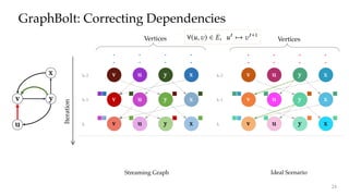
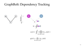
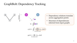
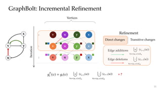
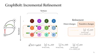
35. y
Refinement: Transitive Changes
k+1
Iteration
k v x
( ).( ) - Combine
pute vertex value for the current iteration. This computation
can be formulated as 2:
ci ( ) =
º
(
8e=(u, )2E
(ci 1(u)) )
where
…
indicates the aggregation operator and
≤
indicates
the function applied on the aggregated value to produce the
nal vertex value. For example in Algorithm 1,
…
is
A on line 6 while
≤
is the computation on line 9. Since
values owing through edges are eectively combined into
aggregated values at vertices, we can track these aggregated
values instead of individual dependency information. By
doing so, value dependencies can be corrected upon graph
mutation by incrementally correcting the aggregated values
and propagating corrections across subsequent aggregations
throughout the graph.
Let i ( ) be the aggregated value for vertex for iteration
i, i.e., i ( ) =
…
8e=(u, )2E
(ci 1(u)). We dene AG = (VA, EA) as
dependency graph in terms of aggregation values at the end
of iteration k:
VA =
–
i 2[0,k]
i ( ) EA = { ( i 1(u), i ( )) :
i 2 [0,k] ^ (u, ) 2 E }
ations progress. For example, Figure 4
values change across iterations in Lab
Wiki graph (graph details in Table 2) fo
dow. As we can see, the color density is
iterations indicating that majority of ver
those iterations; after 5 iterations, values
the color density decreases sharply. As v
corresponding aggregated values also st
a useful opportunity to limit the amount
that must be tracked during execution.
We conservatively prune the depen
balance the memory requirements for
values with recomputation cost during
particular, we incorporate horizontal p
pruning over the dependence graph tha
dierent dimensions. As values start
tal pruning is achieved by directly sto
of aggregated values after certain iter
the horizontal red line in Figure 4 indic
which aggregated values won’t be track
on the other hand, operates at vertex-le
by not saving aggregated values that h
eliminates the white regions above the h
( ).( )
( ) - Transform
y
Vertex aggregation
35

36. y
Refinement: Transitive Changes
k+1
Iteration
k v x
y
vv x
Complex
Aggregation
• Retract : Old value
• Propagate : New value
Incremental refinement
8: A(sum[ ][i + 1], new_de ree[u] )
9: end function
10: function P( )
11: for i 2 [0...k] do
12: M(E_add, , i)
13: M(E_delete, , i)
14: end for
15: V _updated = S(E_add [ E_delete)
16: V _chan e = T(E_add [ E_delete)
17: for i 2 [0...k] do
18: E_update = {(u, ) : u 2 V _updated}
19: M(E_update, , i)
20: M(E_update, , i)
21: V _dest = T(E_update)
22: V _chan e = V _chan e [ V _dest
23: V _updated = M(V _chan e, , i)
24: end for
25: 8s 2 S :
Œ
8e=(u, )2E
(
Õ
8s0 2S
(u,s0) ⇥ (u, ,s0,s) ⇥ c(u,s0) )
26: 8s 2 S :
Œ
8e=(u, )2E
(
Õ
8s0 2S
(u,s0) ⇥ (u, ,s0,s) ⇥
c(u,s0)
c( ,s0) )
27: end function
Belief Propagation
TransformAggregation Vertex Value
( ).( ) - Combine
pute vertex value for the current iteration. This computation
can be formulated as 2:
ci ( ) =
º
(
8e=(u, )2E
(ci 1(u)) )
where
…
indicates the aggregation operator and
≤
indicates
the function applied on the aggregated value to produce the
nal vertex value. For example in Algorithm 1,
…
is
A on line 6 while
≤
is the computation on line 9. Since
values owing through edges are eectively combined into
aggregated values at vertices, we can track these aggregated
values instead of individual dependency information. By
doing so, value dependencies can be corrected upon graph
mutation by incrementally correcting the aggregated values
and propagating corrections across subsequent aggregations
throughout the graph.
Let i ( ) be the aggregated value for vertex for iteration
i, i.e., i ( ) =
…
8e=(u, )2E
(ci 1(u)). We dene AG = (VA, EA) as
dependency graph in terms of aggregation values at the end
of iteration k:
VA =
–
i 2[0,k]
i ( ) EA = { ( i 1(u), i ( )) :
i 2 [0,k] ^ (u, ) 2 E }
ations progress. For example, Figure 4
values change across iterations in Lab
Wiki graph (graph details in Table 2) fo
dow. As we can see, the color density is
iterations indicating that majority of ver
those iterations; after 5 iterations, values
the color density decreases sharply. As v
corresponding aggregated values also st
a useful opportunity to limit the amount
that must be tracked during execution.
We conservatively prune the depen
balance the memory requirements for
values with recomputation cost during
particular, we incorporate horizontal p
pruning over the dependence graph tha
dierent dimensions. As values start
tal pruning is achieved by directly sto
of aggregated values after certain iter
the horizontal red line in Figure 4 indic
which aggregated values won’t be track
on the other hand, operates at vertex-le
by not saving aggregated values that h
eliminates the white regions above the h
( ) - Transform
( ).( ) ( ).( )
Vertex aggregation
36

37. yy
( )( )
v
y
Refinement: Transitive Changes
k+1
Iteration
k v x
y
x
Complex
Aggregation
• Retract : Old value
• Propagate : New value
8: A(sum[ ][i + 1], new_de ree[u] )
9: end function
10: function P( )
11: for i 2 [0...k] do
12: M(E_add, , i)
13: M(E_delete, , i)
14: end for
15: V _updated = S(E_add [ E_delete)
16: V _chan e = T(E_add [ E_delete)
17: for i 2 [0...k] do
18: E_update = {(u, ) : u 2 V _updated}
19: M(E_update, , i)
20: M(E_update, , i)
21: V _dest = T(E_update)
22: V _chan e = V _chan e [ V _dest
23: V _updated = M(V _chan e, , i)
24: end for
25: 8s 2 S :
Œ
8e=(u, )2E
(
Õ
8s0 2S
(u,s0) ⇥ (u, ,s0,s) ⇥ c(u,s0) )
26: 8s 2 S :
Œ
8e=(u, )2E
(
Õ
8s0 2S
(u,s0) ⇥ (u, ,s0,s) ⇥
c(u,s0)
c( ,s0) )
27: end function
Belief Propagation
TransformAggregation Vertex Value
( ).( ) ( ).( )
( ).( ) - Combine
pute vertex value for the current iteration. This computation
can be formulated as 2:
ci ( ) =
º
(
8e=(u, )2E
(ci 1(u)) )
where
…
indicates the aggregation operator and
≤
indicates
the function applied on the aggregated value to produce the
nal vertex value. For example in Algorithm 1,
…
is
A on line 6 while
≤
is the computation on line 9. Since
values owing through edges are eectively combined into
aggregated values at vertices, we can track these aggregated
values instead of individual dependency information. By
doing so, value dependencies can be corrected upon graph
mutation by incrementally correcting the aggregated values
and propagating corrections across subsequent aggregations
throughout the graph.
Let i ( ) be the aggregated value for vertex for iteration
i, i.e., i ( ) =
…
8e=(u, )2E
(ci 1(u)). We dene AG = (VA, EA) as
dependency graph in terms of aggregation values at the end
of iteration k:
VA =
–
i 2[0,k]
i ( ) EA = { ( i 1(u), i ( )) :
i 2 [0,k] ^ (u, ) 2 E }
ations progress. For example, Figure 4
values change across iterations in Lab
Wiki graph (graph details in Table 2) fo
dow. As we can see, the color density is
iterations indicating that majority of ver
those iterations; after 5 iterations, values
the color density decreases sharply. As v
corresponding aggregated values also st
a useful opportunity to limit the amount
that must be tracked during execution.
We conservatively prune the depen
balance the memory requirements for
values with recomputation cost during
particular, we incorporate horizontal p
pruning over the dependence graph tha
dierent dimensions. As values start
tal pruning is achieved by directly sto
of aggregated values after certain iter
the horizontal red line in Figure 4 indic
which aggregated values won’t be track
on the other hand, operates at vertex-le
by not saving aggregated values that h
eliminates the white regions above the h
( ) - Transform
Vertex aggregation Incremental refinement
37

38. Refinement: Aggregation Types
Complex Simple
Aggregation
Propagate : Change in vertex value
y
k+1
Iteration
k v x
y y
vv x
PageRank
Edges Vertices
] 378M 12M
[7] 1.0B 39.5M
1] 1.5B 41.7M
[8] 2.0B 52.6M
14] 2.5B 68.3M
] 6.6B 1.4B
Algorithm Aggregation (
…
)
PageRank (PR)
Õ
8e=(u, )2E
c(u)
out_de ree(u)
Belief Propagation (BP) 8s 2 S :
Œ
8e=(u, )2E
(
Õ
8s02S
(u, s0) ⇥ (u, , s0, s) ⇥ c(u, s0) )
Label Propagation (LP) 8f 2 F :
Õ
c(u, f ) ⇥ wei ht(u, )
TransformAggregation Vertex Value
( ).( ) - Combine
pute vertex value for the current iteration. This computation
can be formulated as 2:
ci ( ) =
º
(
8e=(u, )2E
(ci 1(u)) )
where
…
indicates the aggregation operator and
≤
indicates
the function applied on the aggregated value to produce the
nal vertex value. For example in Algorithm 1,
…
is
A on line 6 while
≤
is the computation on line 9. Since
values owing through edges are eectively combined into
aggregated values at vertices, we can track these aggregated
values instead of individual dependency information. By
doing so, value dependencies can be corrected upon graph
mutation by incrementally correcting the aggregated values
and propagating corrections across subsequent aggregations
throughout the graph.
Let i ( ) be the aggregated value for vertex for iteration
i, i.e., i ( ) =
…
8e=(u, )2E
(ci 1(u)). We dene AG = (VA, EA) as
dependency graph in terms of aggregation values at the end
of iteration k:
VA =
–
i 2[0,k]
i ( ) EA = { ( i 1(u), i ( )) :
i 2 [0,k] ^ (u, ) 2 E }
ations progress. For example, Figure 4
values change across iterations in Lab
Wiki graph (graph details in Table 2) fo
dow. As we can see, the color density is
iterations indicating that majority of ver
those iterations; after 5 iterations, values
the color density decreases sharply. As v
corresponding aggregated values also st
a useful opportunity to limit the amount
that must be tracked during execution.
We conservatively prune the depen
balance the memory requirements for
values with recomputation cost during
particular, we incorporate horizontal p
pruning over the dependence graph tha
dierent dimensions. As values start
tal pruning is achieved by directly sto
of aggregated values after certain iter
the horizontal red line in Figure 4 indic
which aggregated values won’t be track
on the other hand, operates at vertex-le
by not saving aggregated values that h
eliminates the white regions above the h
( ) - Transform
( ).( ) ( ).( )
Vertex aggregation Incremental refinement
38

39. ( )
v
Refinement: Aggregation Types
Complex Simple
Aggregation
y
k+1
Iteration
k v x
y y
x
PageRank
Edges Vertices
] 378M 12M
[7] 1.0B 39.5M
1] 1.5B 41.7M
[8] 2.0B 52.6M
14] 2.5B 68.3M
] 6.6B 1.4B
Algorithm Aggregation (
…
)
PageRank (PR)
Õ
8e=(u, )2E
c(u)
out_de ree(u)
Belief Propagation (BP) 8s 2 S :
Œ
8e=(u, )2E
(
Õ
8s02S
(u, s0) ⇥ (u, , s0, s) ⇥ c(u, s0) )
Label Propagation (LP) 8f 2 F :
Õ
c(u, f ) ⇥ wei ht(u, )
TransformAggregation Vertex Value
Propagate : Change in vertex value
( ).( ) - Combine
pute vertex value for the current iteration. This computation
can be formulated as 2:
ci ( ) =
º
(
8e=(u, )2E
(ci 1(u)) )
where
…
indicates the aggregation operator and
≤
indicates
the function applied on the aggregated value to produce the
nal vertex value. For example in Algorithm 1,
…
is
A on line 6 while
≤
is the computation on line 9. Since
values owing through edges are eectively combined into
aggregated values at vertices, we can track these aggregated
values instead of individual dependency information. By
doing so, value dependencies can be corrected upon graph
mutation by incrementally correcting the aggregated values
and propagating corrections across subsequent aggregations
throughout the graph.
Let i ( ) be the aggregated value for vertex for iteration
i, i.e., i ( ) =
…
8e=(u, )2E
(ci 1(u)). We dene AG = (VA, EA) as
dependency graph in terms of aggregation values at the end
of iteration k:
VA =
–
i 2[0,k]
i ( ) EA = { ( i 1(u), i ( )) :
i 2 [0,k] ^ (u, ) 2 E }
ations progress. For example, Figure 4
values change across iterations in Lab
Wiki graph (graph details in Table 2) fo
dow. As we can see, the color density is
iterations indicating that majority of ver
those iterations; after 5 iterations, values
the color density decreases sharply. As v
corresponding aggregated values also st
a useful opportunity to limit the amount
that must be tracked during execution.
We conservatively prune the depen
balance the memory requirements for
values with recomputation cost during
particular, we incorporate horizontal p
pruning over the dependence graph tha
dierent dimensions. As values start
tal pruning is achieved by directly sto
of aggregated values after certain iter
the horizontal red line in Figure 4 indic
which aggregated values won’t be track
on the other hand, operates at vertex-le
by not saving aggregated values that h
eliminates the white regions above the h
( ) - Transform
( ).( ) ( ).( )
y
Vertex aggregation Incremental refinement
39

40. 20: V _dest = T(E_update)
21: V _chan e = V _chan e [ V _dest
22: V _updated = M(V _chan e, , i)
23: end for
24: M(V _chan e, B, k)
25: end function
Algorithm 2 PageRank - Complex Aggregation
1: function (e = (u, ), i)
2: A(sum[ ][i + 1],
oldpr[u][i]
old_de ree[u] )
3: end function
4: function (e = (u, ), i)
5: S(sum[ ][i + 1],
oldpr[u][i]
old_de ree[u] )
6: end function
7: function (e = (u, ), i)
8: A(sum[ ][i + 1],
newpr[u][i]
new_de ree[u] )
9: end function
10: function P( )
11: for i 2 [0...k] do
12: M(E_add, , i)
13: M(E_delete, , i)
14: end for
15: V _updated = S(E_add [ E_delete)
16: V _chan e = T(E_add [ E_delete)
17: for i 2 [0...k] do
18: E_update = {(u, ) : u 2 V _updated}
21: V _chan e = V _chan e [ V _dest
22: V _updated = M(V _chan e, , i)
23: end for
24: M(V _chan e, B, k)
25: end function
Algorithm 2 PageRank - Complex Aggregation
1: function (e = (u, ), i)
2: A(sum[ ][i + 1],
oldpr[u][i]
old_de ree[u] )
3: end function
4: function (e = (u, ), i)
5: S(sum[ ][i + 1],
oldpr[u][i]
old_de ree[u] )
6: end function
7: function (e = (u, ), i)
8: A(sum[ ][i + 1],
newpr[u][i]
new_de ree[u] )
9: end function
10: function P( )
11: for i 2 [0...k] do
12: M(E_add, , i)
13: M(E_delete, , i)
14: end for
15: V _updated = S(E_add [ E_delete)
16: V _chan e = T(E_add [ E_delete)
17: for i 2 [0...k] do
18: E_update = {(u, ) : u 2 V _updated}
19: M(E_update, , i)
22: V _updated = M(V _chan e, , i)
23: end for
24: M(V _chan e, B, k)
25: end function
Algorithm 2 PageRank - Complex Aggregation
1: function (e = (u, ), i)
2: A(sum[ ][i + 1],
oldpr[u][i]
old_de ree[u] )
3: end function
4: function (e = (u, ), i)
5: S(sum[ ][i + 1],
oldpr[u][i]
old_de ree[u] )
6: end function
7: function (e = (u, ), i)
8: A(sum[ ][i + 1],
newpr[u][i]
new_de ree[u] )
9: end function
10: function P( )
11: for i 2 [0...k] do
12: M(E_add, , i)
13: M(E_delete, , i)
14: end for
15: V _updated = S(E_add [ E_delete)
16: V _chan e = T(E_add [ E_delete)
17: for i 2 [0...k] do
18: E_update = {(u, ) : u 2 V _updated}
19: M(E_update, , i)
20: M(E_update, , i)
5: S(sum[ ][i + 1],
oldpr[u][i]
old_de ree[u] )
6: end function
7: function (e = (u, ), i)
8: A(sum[ ][i + 1],
newpr[u][i]
new_de ree[u] )
9: end function
10: function P( )
11: for i 2 [0...k] do
12: M(E_add, , i)
13: M(E_delete, , i)
14: end for
15: V _updated = S(E_add [ E_delete)
16: V _chan e = T(E_add [ E_delete)
17: for i 2 [0...k] do
18: E_update = {(u, ) : u 2 V _updated}
19: M(E_update, , i)
20: M(E_update, , i)
21: V _dest = T(E_update)
22: V _chan e = V _chan e [ V _dest
23: V _updated = M(V _chan e, , i)
24: end for
25: end function
1
GraphBolt: Programming Model
Direct changes
40

41. 20: V _dest = T(E_update)
21: V _chan e = V _chan e [ V _dest
22: V _updated = M(V _chan e, , i)
23: end for
24: M(V _chan e, B, k)
25: end function
Algorithm 2 PageRank - Complex Aggregation
1: function (e = (u, ), i)
2: A(sum[ ][i + 1],
oldpr[u][i]
old_de ree[u] )
3: end function
4: function (e = (u, ), i)
5: S(sum[ ][i + 1],
oldpr[u][i]
old_de ree[u] )
6: end function
7: function (e = (u, ), i)
8: A(sum[ ][i + 1],
newpr[u][i]
new_de ree[u] )
9: end function
10: function P( )
11: for i 2 [0...k] do
12: M(E_add, , i)
13: M(E_delete, , i)
14: end for
15: V _updated = S(E_add [ E_delete)
16: V _chan e = T(E_add [ E_delete)
17: for i 2 [0...k] do
18: E_update = {(u, ) : u 2 V _updated}
21: V _chan e = V _chan e [ V _dest
22: V _updated = M(V _chan e, , i)
23: end for
24: M(V _chan e, B, k)
25: end function
Algorithm 2 PageRank - Complex Aggregation
1: function (e = (u, ), i)
2: A(sum[ ][i + 1],
oldpr[u][i]
old_de ree[u] )
3: end function
4: function (e = (u, ), i)
5: S(sum[ ][i + 1],
oldpr[u][i]
old_de ree[u] )
6: end function
7: function (e = (u, ), i)
8: A(sum[ ][i + 1],
newpr[u][i]
new_de ree[u] )
9: end function
10: function P( )
11: for i 2 [0...k] do
12: M(E_add, , i)
13: M(E_delete, , i)
14: end for
15: V _updated = S(E_add [ E_delete)
16: V _chan e = T(E_add [ E_delete)
17: for i 2 [0...k] do
18: E_update = {(u, ) : u 2 V _updated}
19: M(E_update, , i)
22: V _updated = M(V _chan e, , i)
23: end for
24: M(V _chan e, B, k)
25: end function
Algorithm 2 PageRank - Complex Aggregation
1: function (e = (u, ), i)
2: A(sum[ ][i + 1],
oldpr[u][i]
old_de ree[u] )
3: end function
4: function (e = (u, ), i)
5: S(sum[ ][i + 1],
oldpr[u][i]
old_de ree[u] )
6: end function
7: function (e = (u, ), i)
8: A(sum[ ][i + 1],
newpr[u][i]
new_de ree[u] )
9: end function
10: function P( )
11: for i 2 [0...k] do
12: M(E_add, , i)
13: M(E_delete, , i)
14: end for
15: V _updated = S(E_add [ E_delete)
16: V _chan e = T(E_add [ E_delete)
17: for i 2 [0...k] do
18: E_update = {(u, ) : u 2 V _updated}
19: M(E_update, , i)
20: M(E_update, , i)
5: S(sum[ ][i + 1],
oldpr[u][i]
old_de ree[u] )
6: end function
7: function (e = (u, ), i)
8: A(sum[ ][i + 1],
newpr[u][i]
new_de ree[u] )
9: end function
10: function P( )
11: for i 2 [0...k] do
12: M(E_add, , i)
13: M(E_delete, , i)
14: end for
15: V _updated = S(E_add [ E_delete)
16: V _chan e = T(E_add [ E_delete)
17: for i 2 [0...k] do
18: E_update = {(u, ) : u 2 V _updated}
19: M(E_update, , i)
20: M(E_update, , i)
21: V _dest = T(E_update)
22: V _chan e = V _chan e [ V _dest
23: V _updated = M(V _chan e, , i)
24: end for
25: end function
1
Transitive changes
41
GraphBolt: Programming Model - Complex aggregations

42. 21: V _chan e = V _chan e [ V _dest
22: V _updated = M(V _chan e, , i)
23: end for
24: M(V _chan e, B, k)
25: end function
Algorithm 2 PageRank - Complex Aggregation
1: function (e = (u, ), i)
2: A(sum[ ][i + 1],
oldpr[u][i]
old_de ree[u] )
3: end function
4: function (e = (u, ), i)
5: S(sum[ ][i + 1],
oldpr[u][i]
old_de ree[u] )
6: end function
7: function (e = (u, ), i)
8: A(sum[ ][i + 1],
newpr[u][i]
new_de ree[u] )
9: end function
10: function P( )
11: for i 2 [0...k] do
12: M(E_add, , i)
13: M(E_delete, , i)
14: end for
15: V _updated = S(E_add [ E_delete)
16: V _chan e = T(E_add [ E_delete)
17: for i 2 [0...k] do
18: E_update = {(u, ) : u 2 V _updated}
19: M(E_update, , i)
22: V _updated = M(V _chan e, , i)
23: end for
24: M(V _chan e, B, k)
25: end function
Algorithm 2 PageRank - Complex Aggregation
1: function (e = (u, ), i)
2: A(sum[ ][i + 1],
oldpr[u][i]
old_de ree[u] )
3: end function
4: function (e = (u, ), i)
5: S(sum[ ][i + 1],
oldpr[u][i]
old_de ree[u] )
6: end function
7: function (e = (u, ), i)
8: A(sum[ ][i + 1],
newpr[u][i]
new_de ree[u] )
9: end function
10: function P( )
11: for i 2 [0...k] do
12: M(E_add, , i)
13: M(E_delete, , i)
14: end for
15: V _updated = S(E_add [ E_delete)
16: V _chan e = T(E_add [ E_delete)
17: for i 2 [0...k] do
18: E_update = {(u, ) : u 2 V _updated}
19: M(E_update, , i)
20: M(E_update, , i)
Algorithm 1 PageRank - Simple Aggregation
1: function (e = (u, ), i)
2: A(sum[ ][i + 1],
oldpr[u][i]
old_de ree[u] )
3: end function
4: function (e = (u, ), i)
5: S(sum[ ][i + 1],
oldpr[u][i]
old_de ree[u] )
6: end function
7: function D(e = (u, ), i)
8: A(sum[ ][i + 1],
newpr[u][i]
new_de ree[u]
oldpr[u][i]
old_de ree[u] )
9: end function
10: function P( )
11: for i 2 [0...k] do
12: M(E_add, , i)
13: M(E_delete, , i)
14: end for
15: V _updated = S(E_add [ E_delete)
16: V _chan e = T(E_add [ E_delete)
17: for i 2 [0...k] do
18: E_update = {(u, ) : u 2 V _updated}
5: S(sum[ ][i + 1],
oldpr[u][i]
old_de ree[u] )
6: end function
7: function D(e = (u, ), i)
8: A(sum[ ][i + 1],
newpr[u][i]
new_de ree[u]
oldpr[u][i]
old_de ree[u] )
9: end function
10: function P( )
11: for i 2 [0...k] do
12: M(E_add, , i)
13: M(E_delete, , i)
14: end for
15: V _updated = S(E_add [ E_delete)
16: V _chan e = T(E_add [ E_delete)
17: for i 2 [0...k] do
18: E_update = {(u, ) : u 2 V _updated}
19: M(E_update, D, i)
20: V _dest = T(E_update)
21: V _chan e = V _chan e [ V _dest
22: V _updated = M(V _chan e, , i)
23: end for
24: end function
Algorithm 2 PageRank - Complex Aggregation
1: function (e = (u, ), i)
2: A(sum[ ][i + 1],
oldpr[u][i]
old_de ree[u] )
3: end function
4: function (e = (u, ), i)
Transitive changes
42
GraphBolt: Programming Model - Simple aggregations

43. GraphBolt Details …
• Aggregation properties non-decomposable aggregations
• Pruning dependencies for light-weight tracking
• Vertical pruning
• Horizontal pruning
• Hybrid incremental execution
• With without dependency information
• Graph data structure parallelization model
43

44. ces
M
M
M
M
M
B
uation.
m B
48)
Hz
GB
B/sec
ion.
Algorithm Aggregation (
…
)
PageRank (PR)
Õ
8e=(u, )2E
c(u)
out_de ree(u)
Belief Propagation (BP) 8s 2 S :
Œ
8e=(u, )2E
(
Õ
8s02S
(u, s0) ⇥ (u, , s0, s) ⇥ c(u, s0) )
Label Propagation (LP) 8f 2 F :
Õ
8e=(u, )2E
c(u, f ) ⇥ wei ht(u, )
Co-Training Expectation Õ
8e=(u, )2E
c(u)⇥wei ht(u, )Õ
8e=(w, )2E
wei ht(w, )
Maximization (CoEM)
Collaborative Filtering (CF) h
Õ
8e=(u, )2E ci (u).ci (u)tr ,
Õ
8e=(u, )2E ci (u).wei ht(u, ) i
Triangle Counting (TC)
Õ
8e=(u, )2E
|in_nei hbors(u) out_nei hbors( )|
Table 4. Graph algorithms used in evaluation and their aggregation functions.
ining Expectation Max-
pervised learning algo-
Collaborative Filtering
ach to identify related
Triangle Counting (TC)
iangles.
aphs used in our evalu-
ed an initial xed point
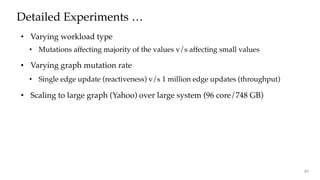
To ensure a fair comparison among the above versions, ex-
periments were run such that each algorithm version had
the same number of pending edge mutations to be processed
(similar to methodology in [44]). Unless otherwise stated,
100K edge mutations were applied before the processing of
each version. While Theorem 4.1 guarantees correctness of
results via synchronous processing semantics, we validated
correctness for each run by comparing nal results.
Experimental Setup
Graphs Edges Vertices
Wiki (WK) [47] 378M 12M
UKDomain (UK) [7] 1.0B 39.5M
Twitter (TW) [21] 1.5B 41.7M
TwitterMPI (TT) [8] 2.0B 52.6M
Friendster (FT) [14] 2.5B 68.3M
Yahoo (YH) [49] 6.6B 1.4B
Table 2. Input graphs used in evaluation.
System A System B
Core Count 32 (1 ⇥ 32) 96 (2 ⇥ 48)
Core Speed 2GHz 2.5GHz
Memory Capacity 231GB 748GB
Memory Speed 9.75 GB/sec 7.94 GB/sec
Table 3. Systems used in evaluation.
Be
La
Co
M
Coll
Tr
Tab
is a learning algorithm while Co-Training Expect
imization (CoEM) [28] is a semi-supervised lea
rithm for named entity recognition. Collaborativ
Server: 32-core / 2 GHz / 231 GB
44

45. 0
10
20
30
40
50
1K 10K 100K
Computationtime
(seconds)
0
50
100
150
200
1K 10K 100K
Computationtime
(seconds)
0
100
200
300
400
500
1K 10K 100K
Computationtime
(seconds)
0
50
100
150
200
1K 10K 100K
Computationtime
(seconds)
0
75
150
225
300
1K 10K 100K
Computationtime
(seconds)
0
20
40
60
80
1K 10K 100K
Computationtime
(seconds)
GraphBolt PerformanceExecutiontimeExecutiontime
ExecutiontimeExecutiontime
Executiontime
Executiontime
0
1
Normalized
computationtime
Ligra
GraphBolt-Reset
GraphBolt
PR on TT( BP on TT
COEM on FT LP on FT TC on FT
CF on TT
45

46. 0
25
50
75
100
1K 10K 100K
%Edge
Computations
0
25
50
75
100
1K 10K 100K
%Edge
Computations
0
5
10
15
20
1K 10K 100K
%Edge
Computations
0
5
10
15
20
1K 10K 100K
%Edge
Computations
0
5
10
15
20
1K 10K 100K
%Edge
Computations
0
0.025
0.05
0.075
0.1
1K 10K 100K
%Edge
Computations
0
4
8
12
16
Computationtime
(seconds)
0
7
14
21
28
Computationtime
(seconds)
0
20
40
60
80
Computationtime
(seconds)
0
10
20
30
40
50
Computationtime
(seconds)
0
25
50
75
100
Computationtime
(seconds)
0
0.5
1
1.5
2
Computationtime
(seconds)
GraphBolt PerformanceExecutiontimeExecutiontime
ExecutiontimeExecutiontime
ExecutiontimeExecutiontime
PR on TT(1.4x to 1.6x) BP on TT (8.6x to 23.1x)
COEM on FT (28.5x to 32.3x) LP on FT (5.9x to 24.7x) TC on FT (279x to 722.5x)
CF on TT (3.8x to 8.6x)
0
1
Normalized
computationtime
GB-Reset
GraphBolt
0
1
Normalized
computationtime
GraphBolt-Reset
GraphBolt
100
100100 100
46

47. 0
10
20
30
40
50
Computationtime
(seconds)
Executiontime
0
4
8
12
16
Computationtime
(seconds)
0
7
14
21
28
Computationtime
(seconds)
0
20
40
60
80
Computationtime
(seconds)
0
0.5
1
1.5
2
Computationtime
(seconds)
0
25
50
75
100
1K 10K 100K
%Edge
Computations
0
25
50
75
100
1K 10K 100K
%Edge
Computations
0
5
10
15
20
1K 10K 100K
%Edge
Computations
0
5
10
15
20
1K 10K 100K
%Edge
Computations
0
5
10
15
20
1K 10K 100K
%Edge
Computations
0
0.025
0.05
0.075
0.1
1K 10K 100K
%Edge
Computations
0
25
50
75
100
Computationtime
(seconds)
GraphBolt PerformanceExecutiontime
ExecutiontimeExecutiontime
ExecutiontimeExecutiontime
LP on FT (5.9x to 24.7x)
0
1
Normalized
computationtime
GB-Reset
GraphBolt
PR on TT(1.4x to 1.6x) BP on TT (8.6x to 23.1x)
COEM on FT (28.5x to 32.3x) TC on FT (279x to 722.5x)
CF on TT (3.8x to 8.6x)
0
1
Normalized
computationtime
GraphBolt-Reset
GraphBolt
100
100100 100
0.2%
3.6%
9.3%
100
100
100
47

48. 0
10
20
30
40
50
Computationtime
(seconds)
0
25
50
75
100
Computationtime
(seconds)
0
0.5
1
1.5
2
Computationtime
(seconds)
0
4
8
12
16
Computationtime
(seconds)
0
7
14
21
28
Computationtime
(seconds)
0
25
50
75
100
1K 10K 100K
%Edge
Computations
0
25
50
75
100
1K 10K 100K
%Edge
Computations
0
5
10
15
20
1K 10K 100K
%Edge
Computations
0
5
10
15
20
1K 10K 100K
%Edge
Computations
0
5
10
15
20
1K 10K 100K
%Edge
Computations
0
0.025
0.05
0.075
0.1
1K 10K 100K
%Edge
Computations
0
20
40
60
80
Computationtime
(seconds)
GraphBolt PerformanceExecutiontimeExecutiontime
ExecutiontimeExecutiontime
ExecutiontimeExecutiontime
CF on TT (3.8x to 8.6x)
0
1
Normalized
computationtime
GB-Reset
GraphBolt
PR on TT(1.4x to 1.6x) BP on TT (8.6x to 23.1x)
COEM on FT (28.5x to 32.3x) LP on FT (5.9x to 24.7x) TC on FT (279x to 722.5x)
0
1
Normalized
computationtime
GraphBolt-Reset
GraphBolt
100
2.1%0.4%
7.8%
100
100
100 100100
48

49. • Varying workload type
• Mutations affecting majority of the values v/s affecting small values
• Varying graph mutation rate
• Single edge update (reactiveness) v/s 1 million edge updates (throughput)
• Scaling to large graph (Yahoo) over large system (96 core/748 GB)
Detailed Experiments …
49

50. GraphBolt v/s Differential Dataflow
0
25
50
75
100
125
150
175
20 40 60 80 100
PR on TT
ExecutionTime(sec)
Single Edge Mutations
Di erential Data ow
GraphBolt
0
25
50
75
100
125
150
175
20 40 60 80 100
ExecutionTime
(seconds)
Single Edge Mutations
0
125
250
375
500
625
1 10 100 1K 10K
ExecutionTime
(seconds)
Batch Size
0
125
250
375
500
625
1 10 100 1K 10K
ExecutionTime
(seconds)
Batch Size
Diferential Data ow
GraphBolt
Differential Dataflow. McSherry et al., CIDR 2013.
PR on TT PR on TT
(100 single edge mutations)
7.6x
41.7x
50

51. Summary
• Efficient incremental processing of streaming graphs
• Guarantee Bulk Synchronous Parallel semantics
• Lightweight dependence tracking at aggregation level
• Dependency-aware value refinement upon graph mutation
• Programming model to support incremental complex aggregation types
Acknowledgements
51
github.com/pdclab/graphbolt