Analyzing Campus Trees and Ecoregion NPP

GEOG 101 Physical Geography
Lab 10: Analyzing Campus Trees and North American
Ecoregions
Name ___________________________________ Lab Section
__________Date __________Materials and sources that will
help you
· Pencil & clip board
· Calculator
· Distance measuring tapes
· Tree diameter (DBH) measuring tapes
· Clinometer
· Internet
Introduction
Think for a moment. How tall is the gingko tree next to Butte
Hall? What about its diameter? You probably look at this tree
almost every day, but have you ever looked up and seen how
tall this tree is? Trees provide shelter for many species as well
as protection to humans. If strategically planted, trees provide
summertime shade and wintertime sunshine to reduce the energy
cost of your home. You can select which species of tree you
would like to plant in order to maximize the shade during the
summertime.
We are seriously concerned about carbon emissions from
various anthropogenic sources. Trees sequester carbon from the
atmosphere via photosynthesis. Sequestered carbon will not be
released back into the atmosphere until trees are decomposed or
burned. A tree’s biomass shows how much carbon has been
sequestered, and the height and diameter of a tree are good
indicators of the biomass. In this lab, you will determine the
height and measure the diameter of three trees on campus. You
will also learn that different ecoregions are associated with
different amounts of biomass.

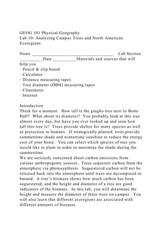
Section 1 – Campus Trees Analysis
Make sure to read the following website before coming to the
lab 10.
Forest Canopy Heights Across the United States
http://earthobservatory.nasa.gov/IOTD/view.php?id=44717
In this section, you will estimate tree heights and measure DBH
(diameter at breast height) values. In order to estimate the
height of a tree, you will use a clinometer and a tape measure.
Figure 1: Data required to estimate the height of an object
In order to estimate the height of a tree, you need to measure
three values (Figure 1):
E: an observer’s eye height from the ground (in meters);
D: a distance from a tree to the observer (in meters); and
α: the angle of the top of the tree from the observer’s eye height
(in degrees).
You will use a tape measure (in meters) for the values of E and
D, while you use a clinometer (in degrees) for the value of α.
Additionally, you will use a DBH tape to measure the diameter
of a tree at breast height.
“Diameter at breast height, or DBH, is the standard for
measuring trees. DBH refers to the tree diameter measured at
4.5 feet above the ground.” See the illustration below (Figure
2) for details.
(https://www.portlandoregon.gov/trees/article/424017)

Figure 2: Measuring height of the DBH value
(https://www.portlandoregon.gov/trees/article/424017)
Form a group of 4-5 members so that there is a total of five
groups. Alternatively, you can form a group with members
whom you collected temperature data along a designated path
(Lab 4).
Before you start collecting data to estimate tree heights, assign
one group member who will measure the angle (α). Then you
will then measure this group member’s eye-level height (E)—
from the ground to this group member’s eye level.
The observer’s eye height (E) is _____varies_____ m.
This height (E) is probably measured in meters and centimeters.
Convert your reading so that this height (E) is in meters. For
example, if this height (E) is 1 meter and 58 cm, then this value
in meters is 1.58 m. Remember that 1 m = 100 cm.
1) We will first gather and practice how to estimate tree height
and measure a DBH value on the south side of Butte Hall. Your
instructor will show you how to set up your devices.
E: an observer’s eye height from the ground: ___varies_______
m
D: a distance from a tree to the observer: _____varies_____ m
α: the angle of the top of the tree from the observer’s eye
height: _____varies_____ degrees
2) Calculate the tree height using the data you just collected.

You will use the following equation.
Height (in meters) = D x tan(α) + E
Use the calculator on your smartphone to calculate the height of
this tree.
The height of this practice tree is: ____varies______ m
3) Now your instructor will show you how to use the DBH tape
to measure the tree diameter at breast height.
The diameter at breast height is: ____ varies ______ cm
Circumference at breast height is:_varies __cm. Divide by 100
to find meters:__ varies ______m
4) Go to a designated location and estimate the height and
measure the DBH value of a predetermined tree.
Eye-height (E in meters)
Distance (D in meters)
Angle (α in degrees)
Tree height (m)
varies
DBH (in centimeters)
Circumference (in meters)
Notes
varies
5) Your group will select one additional nearby tree and repeat
this exercise. Use a smartphone and take a picture of the tree
(and you will show it to your instructor upon returning to the
classroom).
Eye-height (E in meters)

Distance (D in meters)
Angle (α in degrees)
Tree height (m)
varies
DBH (in centimeters)
Circumference (in meters)
Notes
varies
6) Report estimated tree heights and measured DBH values.
7) Your instructor will plot the data using Excel to show you
the relationship between the tree heights and DBH values.
Before DBH and tree heights are plotted, form a hypothesis
regarding the relationship between these two values.
For the trees on the CSU Chico campus, as DBH increases,
height also increases.
I think this is a positive, linear relationship
8) Is your hypothesis rejected or not rejected? Is it a linear or
non-linear relationship? Is it positive or negative relationship?
I was right! Tree height increases as DBH increases in a
positive, linear relationship
9) Use the chart provided to determine the amount of carbon
(C) in your tree:_________varies________kg
10) Multiply your answer to #9 by 3.6663 to determine the
amount of carbon dioxide (CO2) sequestered by your tree over
the course of its lifetime:
___________ varies ________________kg
11) A round-trip drive from Chico to Los Angeles in an average
car emits about 1030 lbs of carbon dioxide. How does this

number compare to the amount of carbon dioxide your tree has
sequestered? Do you think that planting trees is the answer to
reducing excess carbon dioxide in our atmosphere? Explain.
Apparently, planting trees alone is not the answer to how to
remove carbon dioxide from the environment. The amount of
CO2 sequestered by a tree in its lifetime can be cancelled out by
the CO2 emissions produced by just a few car trips.
Section 2 – Ecoregions and Net Primary Productivity
7.0
6.0
Figure 1 – Ecoregions (level 1) of North America
Source:
ftp://ftp.epa.gov/wed/ecoregions/cec_na/NA_LEVEL_I.pdf
Figure 2 – NPP of Biomes
Source:
http://www.nature.com/scitable/knowledge/library/terrestrial-
primary-production-fuel-for-life-17567411
5
The Net Primary Productivity (NPP) of any location describes
the net photosynthesis taking place. Biomass is a physical
representation of that photosynthesis and displays the difference
between Gross Primary Productivity (GPP) and NPP. GPP
minus respiration by plants is equal to NPP. In other words,
NPP represents the amount of stored energy generated by plants,
and is measured in terms of how much carbon is “fixed” during
the photosynthetic process. NPP can be calculated for any
geographic region. It is usually expressed as a rate, such as
grams or tons of carbon per hectare per year. Keep in mind that
as leaves fall off trees, some of that biomass is being lost to
decomposition. Also, a portion of the productivity of plants is

found belowground in the form of roots.
Source:
http://www.nature.com/scitable/knowledge/library/terrestrial-
primary-production-fuel-for-life-17567411
For this exercise, we will be connecting ecoregion types found
in the contiguous United States with their associated level of
NPP.
1.) In the spaces provided below, complete the following:
· For each of the listed cities, determine that location’s
ecoregion by first finding the city using a laptop, phone, or
tablet and some kind of mapping app. (Any map app will work,
like google maps or apple maps). Next you need to analyze
Figure 1 above along with the descriptions of each ecoregion
and determine which ecoregion each city falls within.
· Once the location has been found, use the ecoregion packet
provided by your instructor to determine the biome listed in
Figure 2 in which the ecoregion fits. Use this information to
determine that ecoregion’s Net Primary Productivity (NPP) in
grams of carbon per hectare per year. (It’s the third column in
the table Figure 2)
2.) Does latitude alone determine the ecoregion of a location?
What other environmental factors must be considered?
Latitude alone does not determine the ecoregion of a location.
Elevation, soil types, and weather
patterns—such as annual precipitation—are also factors in
determining the ecoregion of a location.
1.) City: Portland, Oregon

Ecoregion:______Temperate Forest____________
NPP: 465 - 741 gC/ha-1yr
2.) City: Chico, California
Ecoregion:______Temperate Grasslands______
NPP: 129 – 342 gC/ha-1yr
3.) City: Kansas City, Kansas
Ecoregion:_____Croplands______
NPP: 288 - 468 gC/ha-1yr
4.) City: Indianapolis, Indiana
Ecoregion:_____Croplands________
NPP: 288 - 468 gC/ha-1yr
5.) City: Las Vegas, Nevada
Ecoregion:___Desert______________
NPP: 28 – 151 gC/ha-1yr
6.) City: Miami, Florida
Ecoregion:_____Tropical Forest________
NPP: 871 - 1098 gC/ha-1yr
7.) City: Flagstaff, Arizona
Ecoregion:________ Temperate Forest _______
NPP: 465 - 741 gC/ha-1yr
8.) City: Tuscon, Arizona
Ecoregion:_______Desert_______
NPP: 28 - 151 gC/ha-1yr
9.) City: Missoula, Montana
Ecoregion:_____ Temperate Forest ______
NPP: 465 - 741 gC/ha-1yr
10.) City: Montpelier, Vermont
Ecoregion_____ Temperate Forest ______
NPP: 465 - 741 gC/ha-1yr
LAB 8: Soils and their Analysis
(modified from Shankman with further additions and major

modifications by D. Fairbanks)
Name ANSWER KEY Lab Section __________ Date
_______
Materials and sources that will help you
· Soil samples
· Munsell color chart
· Soil texture analysis kit
· Soil dispersion reagent
· Water
· pH meter and distilled water
· 500ml beakers
· Classroom clock or a watch
Introduction
Soil is a dynamic natural material composed of fine decomposed
mineral and organic matter particles in which plants grow. The
soil system includes human interactions and supports all human,
other animal, and plant life. If you have ever planted a garden,
tended a house plant, or been concerned about famine and soil
loss, this lab exercise will interest you.
Soil science is interdisciplinary, involving physics, chemistry,
biology, mineralogy, hydrology, climatology, and cartography.
Physical geographers are interested in the spatial patterns
formed by soil types, the environmental factors that interact to
produce them, and their effect on plants, animals, human health
and the built environment. Pedology concerns the origin,
classification, distribution, and description of soil. Edaphology
focuses on soil as a medium for sustaining higher plants.
Edaphology emphasizes plant growth, fertility, and the
differences in productivity among soils. Pedology gives us a
general understanding of soils and their classification, whereas
edaphology reflects society's concern for food and fiber
production and the management of soils to increase fertility and

reduce soil losses.
This lab will give you the opportunity for some hands-on
experience with soils, and for using some of the tools and
methods that soil scientists use in their work.
Keywords:
clay
edaphology
humus
loam
pH (acidity-alkalinity)
pedology
permeability
polypedon
porosity
sand
silt
soil
soil classification
soil color
soil consistence
soil horizon
soil profile
soil properties
soil texture
Objectives
· Identify basic components of soil and soil properties.
· Determine main components of soil sample by color.
· Identify major soil texture categories and classify soils by
texture.
· Measure pH level in soil samples and determine the soil pH
(acidity or alkalinity).

Section 1: Soil Texture and Soil Structure
Soil texture refers to the mixture of sizes of its individual
particles and the proportion of different sizes of soil separates
(individual particles of soil). Particles smaller than gravel are
considered part of the soil, while larger particles, such as
gravel, pebbles, or cobbles are not. If you have been to a beach,
you have felt the texture of sand: It has a “gritty” feel. Silt, on
the other hand, feels smooth—somewhat soft and silky, like
flour used in baking bread. When wet, clay has a sticky feel
and requires quite a bit of pressure to squeeze it, like the clay
used in making pottery.
Soils nearly always consist of more than one particle size. By
determining the relative amounts of sand, silt, and clay in a
particular soil sample, it can be placed into one of twelve
classes as shown in the soil texture triangle. Each side presents
percentages of a particle grade. See the line from each side of
the triangle (following the direction indicated by the orientation
of the numbers on each axis). You see that a soil consisting of
36% sand, 43% silt, and 21 % clay is classified as loam, a term
for soils consisting of mostly sand and silt with a relatively
smaller amount of clay. Soils that represent the best particle
size mix for plant growth are those that balance the three sizes.
1. Use the soil texture triangle on the last page of this lab to
name the following by its correct texture class.
a) 17% sand, 28% silt, 55% clay: CLAY
b) 31% sand, 55% silt, 14% clay: SILT LOAM

Part I:
The following is a quantitative approach to measure soil
texture. Here you will use a soil texture kit consisting of a set
of three graduated cylinders, water, a dispersing reagent and a
soil sample to be chosen by your lab instructor. This method
uses the same principle as standard scientifically more accurate
methods (ones you would find a soil analysis lab): the rate of
settling of soil particles in water.
Step 1: Break up into lab pairs of two and go and get the soil
separation tubes and rack, and a graduated cylinder from the
back storage cupboards. Go and fill the graduated cylinder to
the 50 ml line.
Step 2: At the front of the lab your lab instructor will give you
your assigned soil sample. Add the soil sample that your lab
instructor assigned to your group to soil separation Tube “A”
until it is even with line 15. Note: Gently tap the bottom of the
tube on a firm surface to pack the soil and eliminate air spaces.
Step 3: At the front of the lab your lab instructor will have
chemicals for your use. Use a dropper to add 1 ml of texture
dispersing reagent to the sample in soil separation Tube “A”.
Fill Tube “A” with your water from graduated cylinder to line
45.
Step 4:Cap and gently shake for 2 minutes, making sure the soil
sample and water are thoroughly mixed.
The sample is now ready for separation. The separation is
accomplished by allowing a predetermined time for each
fraction to settle out of the solution.
Step 5: Place soil separation tube “A” in the rack. Allow to

stand undisturbed for exactly 30 seconds.
Step 6: Carefully pour off all the solution into soil separation
tube “B”. Return Tube “A” to the rack. Allow Tube “B” to
stand undisturbed for 30 minutes.
Step 7: Carefully pour off the solution from soil separation tube
“B” into soil separation tube “C”. Return Tube “B” to the rack.
While tube “C” would have the suspended clays in a soil, we do
not need it to calculate the percentage sand, silt and clay, as
having the results of tube “A” (sand) and tube “B” (silt)
fractions and subtracting this total from the initial volume of
soil used for the separation is sufficient.
EXAMPLE:
Tube “A” Sand 2 Initial volume 15
+ Tube “B” Silt +8– Total “A” & “B” –10
Total “A” & “B” 10 Clay 5
Step 8: Read soil separation tube “A” at top of soil level. To
calculate percentage sand in the soil, divide reading by 15 and
then multiply it by 100.
Step 9: Read soil separation tube “B” at top of soil level. To
calculate percentage silt in the soil, divide reading by 15 and
then multiply it by 100.
Step 10: Calculate volume of clay as shown above. To calculate
percent clay in the soil, divide value by 15 and then multiply it
by 100.
Sample ID
Percentage
Textural classification

Sand
Silt
Clay
Answers will vary
Divide students into pairs and provide one sample from one of
the sites. There will be duplication of sites being analyzed.
Your lab instructor will record all the class samples on the
board. You should record them and calculate the textural
averages for each sample.
Sample ID
Sand (%)
Silt (%)
Clay (%)
Answers vary with section
Sample ID
Sand (%)
Silt (%)
Clay (%)
3
Answers vary with section
3
3
AVERAGE
4
4
4

AVERAGE
5
5
5
AVERAGE
Answer the following questions based on the data analyzed by
the entire class.
1) Which of the samples has the largest pore spaces?
(The sample with the highest sand content)
2a) Which of the samples has the highest infiltration capacity?
(The sample with the highest sand content
2b) Which of the samples has the lowest infiltration capacity?
The sample with the highest clay content
2c) Explain why?
Clay reduces infiltration capacity.
3a) Which of the samples has the highest water holding
capacity?
(The sample with the highest clay content)
3b) Which of the samples has the lowest water holding
capacity?

(The sample with the highest sand content)
3c) Explain why?
Sand reduces water holding capacity.
Part II.
In a less quantitative way, soil texture can be determined in the
field by feeling the soil and estimating the percentages of sand,
silt, and clay. Try this method using the following procedure
with a new soil sample, recording your observations and results
through each of these steps.
Step 1: Follow the handout that accompanies the last page of
this lab. Your lab instructor will fill your palm with a dry soil
sample, moistening it with enough water so that it sticks
together sufficiently to be worked with your fingers. Add the
water gradually. If it becomes too runny or if it sticks to your
fingers, add more dry soil. You want a “plastic” mass that you
can mold, somewhat like putty.
Step 2: Follow the remainder of the handout to determine soil
texture.
Record your observations in the space provided. Once you have
a simplified named textural classification review the soil texture
triangle and work out the percentage ranges for sand, silt and
clay.
Name according to handoutResults will vary
Sand _________Depends on your answer above

Silt _________ Depends on your answer above
Clay _________ Depends on your answer above
Section 2: Soil Color
Soil properties are their characteristics, some of which include
soil color, texture, structure, consistence, porosity, moisture,
and chemistry. We examine a few of these properties,
beginning with color.
Soil color is one of the most obvious traits, suggesting
composition and chemical makeup in mineral soils. If you look
at exposed soil, color may be the most obvious trait. Among
the many possible hues are:
· the reds and yellows (high in iron oxides, its rusting);
· the dark browns to blacks (richly organic);
· white-to-pale hues (silicates and aluminum oxides);
· Gray and greenish-bluish (reduced iron from being inundated
in water) and;
· White color (calcium carbonate or other water-soluble salts).
However, color can be deceptive. Soils of high humus content,
organic materials from decomposed plant and animal litter, are
often dark, yet clays of warm-temperate and tropical regions
with less than 3% organic content are some of the world’s
blackest soils.
To standardize color descriptions, soil scientists describe a
soil’s color by comparing it with a Munsell Color Chart. These
charts display colors arranged by:
· Hue (H, the dominant spectral color, such as red),
· Value (V, degree of darkness or lightness), and
· Chroma (C, purity or saturation of the color, which increase
with decreasing grayness).
The complete Munsell notation for a chromatic color is written
symbolically like this: H V/C. As an example, for a strong red

having a hue of 5R (R denoting red), a value of 6, and a chroma
of 14, the complete Munsell notation is 5R 6/14. Another
example, a pale brown is 10YR 6/3 (YR denoting yellow-red).
A dark brown is noted as 10YR 2/2. More refined divisions of
any of the attributes, use decimals.
The light you use when you view the sample is important and
can affect your assessment of the color notation. It is best to
view the chart and the sample with the Sun over your shoulder
shining on the sample, with you facing away from the Sun.
Under artificial classroom light you will find low values and
low chromas—the most difficult to match against the color
chips.
Using soil samples assigned to your group note the predominant
soil color and indicate the likely soil component responsible for
the color. Be sure and note whether the sample is wet, moist, or
dry.
Sample ID
Munsell color
Soil component creating the color
Moisture level
Answers will vary.
Very dry
Note: When doing actual fieldwork with a soil (the complete
soil profile and basic sampling unit in soil surveys), you will
find different colors in each horizon, and maybe more than one
color in a single horizon. These details, in an assessment,
would be noted.
Section 3: Soil Acidity and Alkalinity
Soil fertility is strongly affected by soil acidity or alkalinity as
expressed on the pH scale. Nutrient availability is low in soils
that are either very acidic or very alkaline. A soil solution may

contain significant hydrogen ions (H+), the cations that
stimulate acid formation. The result is a soil rich in hydrogen
ions, or an acid soil. On the other hand, a soil high in base
cations (calcium, magnesium, potassium, sodium) is a basic or
alkaline soil.
Pure water is nearly neutral, with a pH of 7.0. Readings below
7.0 represent increasing acidity. Readings above 7.0 indicate
increasing alkalinity. Acidity usually is regarded as strong at
5.0 or lower, whereas 10.0 or above is considered strongly
alkaline. Several factors influence soil acidity. The chemistry
of soil parent materials, as well as any added fertilization or
removal of plants can increase soil acidity. However, the major
contributor to soil acidity in this modern era is acid
precipitation (rain, snow, fog, or dry deposition). Acid rain
actually has been measured below pH 2.0 – an incredibly low
value for natural precipitation, as acid as lemon juice.
Increased acidity in the soil solution accelerates the chemical
weathering and depletion rates of some mineral nutrients, yet it
can also decrease the availability of other nutrients. Because
most crops are sensitive to specific pH levels, acid soils below
pH 6.0 require treatment to raise the pH. This soil treatment is
accomplished by the addition of bases in the form of minerals
that are rich in base cations, usually lime (calcium carbonate,
CaCO3).
1) Your lab instructor will have five beakers representing the
five soil samples with the addition of distilled water to them on
his/her desk. Using the pH meter provided dip it into each
sample and record the pH level. Make sure to clean off the
meter each time in the clean water beaker before dipping into a
new soil pH test beaker.
Sample ID
pH
1
Answers will vary by section

2
3
4
5
2) Are any of the class samples strongly acidic? If any were,
what remedial actions could be taken to make them more pH
neutral and under what circumstances might you want to do
this? Hint: what does one take for heartburn?
pH numbers vary with section. An acidic soil could be made
more neutral by adding a base, such as crushed limestone.
Soil Texture Triangle
8
1
LAB 7: Earth Materials and Plate Tectonics
(modified from Anderson et al., Christopherson, and the
Southern California Earthquake Center with major
modifications by D. Fairbanks)

Name ANSWER KEY Lab Section Date
• Calculator
• a square piece of card or paper on which you can mark
distances
• a compass for drawing circles
• Internet connection: Google Earth
Key Terms:
asthenosphere
continental
drift core
crust
effusive
eruption hot
spots mantle
mid-ocean
ridges
orogenesis
Pangaea
plate tectonics
plumes
sea-floor spreading
seismic waves
subduction zone
transform faults
shield volcano
composite volcano
rock cycle

Introduction
Plate tectonics theory was a revolution in twentieth century
Earth science. The past few decades have seen profound
breakthroughs in our understanding of how the continents and
oceans evolved, why earthquakes and volcanoes occur
where they do, and the reasons for the present arrangement and
movement of landmasses. One task of physical geography
is to explain the spatial implications of this knowledge and its
effect on Earth’s landforms and human society.
As Earth solidified, heavier elements slowly gravitated toward
the center, and lighter elements slowly welled upward
to the surface, concentrating in the crust. Earth’s interior is
highly structured, with uneven heating generated by the
radioactive decay of unstable elements. The results of this
heating and instability are irregular patterns of moving,
warping, and breaking of the crust.
Preview the following video then proceed with the laboratory
assignment:
http://www.youtube.com/watch?v=QDqskltCixA
Section 1: Earths Internal Structure and Rock cycle
Earthquakes occur because the Earth’s surface is broken up into
approximately 15 rigid plates that collide, pull apart, and
grind past one another. These plates make up Earth's
lithosphere, which includes both the crust (the thin, outermost
layer

of the earth) and the rigid upper portion of the mantle. The
plates are a variety of different sizes and shapes. Some, like the
Pacific Plate, are found entirely underneath ocean basins,
whereas others, like the North American Plate, include parts of
both continents and the ocean floor. The thickness of the plates
varies as well: portions of plates can be anywhere from 5
to 60 kilometers thick. Beneath the plates lies the soft, easily
deformed asthenosphere. The weak asthenosphere allows the
rigid plates to move around above it.
The rock cycle, through processes in the atmosphere, crust, and
mantle, produces three basic rock types – igneous,
sedimentary, and metamorphic. The tectonic cycle brings heat
energy and new materials to the surface and recycles old
materials to mantle depths, creating movement and deformation
of the crust.
2
1. Using the California Geology map handed out to you,
determine the geomorphic province of California that is
composed of a majority of the following rock types.
a. Sedimentary rocks?
Great Valley Province
b. Igneous rocks?
Sierra Nevada Province, Cascade Range Province, Modoc
Plateau Province
c. Metamorphic rocks?

Klamath Mountains Province
2. The legend on the geology map indicates eons, eras and
periods for the rock units. The following table lists the
approximate dates associated with these eons, eras and periods.
a. What type of rock represents the oldest on the map (igneous,
sedimentary or metamorphic)? What geomorphic province
are they found in?
Metamorphic; Klamath Mountains, Basin and Range, Sierra
Nevada, Mojave Desert
b. What type of rock represents the youngest on the map
(igneous, sedimentary or metamorphic)? What geomorphic
province are they found in?
Sedimentary; Great Valley
Section 2: Earthquake Faults and Seismic Activity
Plate boundaries come in three different types: convergent
(where plates move towards one another, such as in the
Himalayas, beneath Japan, or on the Pacific coast of South
America), divergent (where plate pull apart from one another,
such as along the Mid-Atlantic Ridge), and transform (where
plates slide horizontally past one another, such as along the
San Andreas Fault in California).
Convergent/Compression Divergent/Tension Transform

3
Earthquakes occur when rocks suddenly slide past one another
along faults. Most earthquakes occur along faults near
plate boundaries, releasing the energy built up over tens,
hundreds or thousands of years, during which the plates tried to
move, but remained stuck. Seismologists (scientists who study
earthquakes) are still unable to predict when an earthquake
is likely to occur, but they are very good at predicting where
earthquakes are likely. However, there have been some large
earthquakes in the middle of plates, usually along weak zones
that were plate boundaries in the distant past (i.e. New
Meridian fault along the Mississippi river near St. Louis, MO).
The size of an earthquake depends mostly on the size of the
fault that slipped. The enormous (M 9+) earthquake that
occurred in Indonesia on December 26, 2004, generating a
catastrophic tsunami, ruptured 1200 to 1300 kilometers (750
miles) of the plate boundary between the Indian Plate and
Indonesia. In comparison, the 1906 San Francisco earthquake
(M 7.8) was caused by slip along 430 kilometers (267 miles) of
the San Andreas Fault, which forms the boundary
between the North American and Pacific Plates. Larger
earthquakes also occur when the two sides of the fault slip
longer
distances past one another: Indonesia moved approximately 15
meters (50 feet) compared with the Indian Ocean floor,
whereas North America only moved 3 to 6 meters (10 to 20 feet)
past the Pacific Plate.
In all earthquakes, energy is released as the two sides of the
fault slide past one another. This energy, which generates the
ground shaking that causes much of the damage during

earthquakes, is carried through rock by seismic waves. Seismic
waves come in two forms: body waves and surface waves. Body
waves move through the Earth’s interior, and travel
much more quickly than surface waves. Surface waves move
over the surface of the Earth, and cause much of the
destruction during earthquakes.
Body Waves
P waves (also known as primary or compressional waves) are
the first seismic waves to arrive at an earthquake recording
(seismograph) station after an earthquake occurs. Primary waves
behave much like sound waves, traveling through both
solid and liquid layers of the Earth by compressing and
stretching the rocks through which they travel. P waves travel
as
fast as 5.5 km/second, or more than 12,000 miles per hour,
depending on the type of substance through which they travel.
Because P waves travel in a linear motion, there is little
displacement of Earth materials. Primary waves are the least
damaging of all seismic waves.
S waves (also known as secondary or shear waves) are a second
type of body wave. S waves travel in a serpent-like
motion, changing both the shape and volume of rock as they
travel through it. Unlike P waves, S waves can only travel
through solid rock; S waves cannot travel through liquids. In
fact, S waves are one of the main things that tell us that the
Earth has a liquid outer core: no S waves are recorded on the
directly opposite side of Earth from an earthquake. S waves
travel more slowly than P waves, reaching a maximum velocity
of about 3 km/second; when an earthquake occurs, a
seismograph records a P wave first, then an S wave. S waves
can be more damaging than P waves.
The farther a seismograph station is from an earthquake
epicenter, the longer it will take for seismic waves to arrive.

The
time lag between the first shaking due to P waves and due to S
waves also increases with distance from the epicenter. This
time lag allows seismologists to precisely calculate the distance
between an epicenter and their seismograph stations, and
to determine the location of the epicenter. You will determine
an epicenter location by hand later in this lab; computers
follow a similar procedure to locate real earthquakes.
Both types of body waves shake with high frequencies (that is,
they shake rapidly). The high frequencies of body waves
are often similar to the natural frequencies of short buildings
and other structures. As the frequencies of body waves
approach the natural frequencies of buildings, the buildings
begin to vibrate; if the frequency of the seismic waves
matches the “resonant frequency” of the building, the building
may collapse. The amount of shaking increases towards the
top of tall buildings, in a fashion similar to the child’s game
“Crack the Whip,” where the greatest amount of energy is felt
at the end of the line.
The intensity of shaking caused by body waves decreases away
from the epicenter, in the same way that loud sounds seem
quieter the farther you are from the source. This causes the
worst damage, in general, to occur nearest the epicenter of an
earthquake. However, shaking is typically quite intense all
along the fault, and many other factors (including the type of
ground supporting a building and the materials from which a
building is constructed) also contribute to the amount of
damage that occurs.
4

Surface Waves
Surface waves are seismic waves that travel along the earth’s
surface, rather than through solid bodies of rock. There are
two types of surface waves: Rayleigh waves and Love waves.
Both types of waves travel more slowly than body waves,
and both types of waves are more destructive than both P and S
waves, in part because they have lower frequencies, which
are similar to the natural frequencies of tall buildings.
Rayleigh waves, named after Lord Rayleigh, an English
physicist, travel in a backwards elliptical motion, much like the
upwards uncoiling of a spring or the rolling motion of an ocean
wave. Rayleigh waves are the last to arrive at a location
distant from the epicenter.
Love or L waves, named after English mathematician A.E.H.
Love, are horizontal, transverse waves that travel across the
surface of the Earth. Like a snake, these type of waves move
forward as energy is distributed from side to side.
The intensity of vibrations and, therefore, the damage caused by
both surface and body waves, often depends on the type
of soil and rock material on which a building sits. Buildings
constructed on bedrock usually sustain little damage from an
earthquake. Buildings, structures, and cities built on
unconsolidated or loose material such as sand, silt, and clay are
often
subject to devastating loss of property and human lives. Loose
or unconsolidated Earth materials often magnify the
intensity of seismic waves.
3. Each group take a metal coil and have two students take an
end, stretch it and then have one of the students push it

towards their partner without releasing the end. Describe how
the energy moves through the coil. What type of seismic
wave was created?
Primary (P) waves
4. Next, have your partner hold the end of the metal coil so that
it doesn’t move. Wiggle your end up and down several
times. Note that the source of the vibration is moving up and
down vertically What do you observe about the motion of
the wave as it travels through the metal coil? What type of
seismic wave was created?
Secondary (S) waves
5. Lastly, you and your partner should stretch out the coil onto a
tabletop and then have one of you wiggle the end from
side to side while the other partner holds the other end of the
metal coil so that it doesn’t move. Note that the source of the
vibration is moving horizontally. What do you observe about the
motion of the wave as it travels through the metal coil?
What type of seismic wave was created?
Love (L) waves
6. The understanding of the composition of the Earth’s interior
is an example of scientific limitations. How have scientists
established this portrait of Earth’s interior since no one has ever
sampled the interior below the crust directly? Explain.
Scientists gain a picture of the Earth’s interior by measuring the
speed and direction of different seismic waves as
the travel, as well as how speed and direction of these waves
change over time.
Primary or P-waves

5
Earthquake Size
The size of an earthquake can be measured in two ways:
intensity and magnitude.
• Intensity of an earthquake measures the effect of an
earthquake on people, objects, and structures, and is
determined by reports of people who experienced the
earthquake. (If you feel an earthquake, you can help
determine its intensity by filling out a questionnaire for the U.S.
Geological Survey at
http://earthquake.usgs.gov/earthquakes/dyfi/ )
• Magnitude (measured on a logarithmic scale referred to in the
news as the “Richter scale”) is measured based on
a seismograph’s record of the amount of shaking during an
earthquake. A traditional seismograph consists of a
free weight suspended from a wire attached to a support, which
is anchored to the ground. A pen is attached to the
weight. As the ground shakes, the pen traces a jagged line on
the paper below it. The farther the pen moves (and
the larger the wobbles recorded on the paper), the higher the
amplitude of shaking. Amplitude of shaking is
converted to Richter scale magnitude by correcting for distance
from the epicenter and taking the logarithm of the
amplitude. The resulting magnitudes reflect a 10-fold increase
in strength for every one-fold increase in Richter
magnitude. An earthquake registering a magnitude 6 is 10 times
stronger than magnitude 5, 100 times stronger
than magnitude 4, 1000 times stronger than magnitude 3, and

10,000 times stronger than magnitude 2.
Magnitudes greater than 7 are classified as major earthquakes,
capable of causing mass destruction and death.
7. Go to the following website:
http://earthquake.usgs.gov/earthquakes/map/ click on this icon
in the
upper right hand corner of the web page. This will allow you to
modify the map:
a. Select 30 Days, magnitude 4.5+, worldwide, then zoom out so
you can see the Pacific Ocean.. What does the seismic
activity map tell us about plate tectonics in the Pacific region?
Seismic activity is generally located along the plate boundary
b. Select 30 days, magnitude 2.5+ worldwide, and zoom to just
the continental US. . What does the seismic activity map
tell us about the Western USA?
Seismic activity is generally located on the plate boundary, and
specifically along the San Andreas Fault
c. Zoom the map to just Hawaii. Why is the seismic activity
mostly recorded only on the Big Island of Hawaii?
The Pacific Plate is slowly moving northwest, with a “hotspot”
that is presently located below the Big Island. As
the plate continues to move in this direction, the stationary “hot
spot” beneath the plate will cause more volcanic
islands will form in a row on the southeastern part of the chain.
(Imagine a piece of paper slowly moving over a
stationary flame, resulting in a charred line across the paper)

8. Go to the following website:
http://earthquake.usgs.gov/earthquakes/dyfi/ and look at the
following historic event
maps of intensity:
• Loma Prieta, CA October 18, 1989 (click “View Archives” and
type in the search field: Loma Prieta 1989-10-18)
• Near Reseda, CA Jan 17, 1994 (likewise, type in the search
field: Northridge).
While the Reseda earthquake (known in the media as the
Northridge earthquake) was slightly smaller than the Loma
Prieta earthquake, the Northridge quake had more intensity
recorded than the Loma Prieta. Explain why this is using the
two maps and your general knowledge of California geography
(we did not get to this answer in class)
6
Section 3: Locating the Epicenter of an Earthquake
When an earthquake occurs, it releases seismic waves that can
be detected at stations all around the globe. Remember that
there are three types of waves released by an earthquake:
primary, secondary, and surface waves. Primary waves (P-
waves) travel via compression and are the first to arrive at
seismic stations. They generally travel at a rate between 5.95
and 6.75 kilometers per second (km/sec), depending on various
factors in the crust including density, compressibility, and
rigidity. Secondary waves (S-waves) have a shearing motion
and are the second type of wave to be detected, traveling
between 2.9 and 4.0 km/sec. The last waves to arrive are the
surface waves (L-waves), which have velocities around 2.7

and 3.7 km/sec.
Geographers and geologists can use these known travel times to
approximate the distance from the reporting station to the
epicenter. Three or more stations can compare their distances to
the epicenter in order to determine its exact location –
known as triangulation.
Let’s assume that you work at the seismic reporting station in
Golden, Colorado. At 1:45pm you receive the first P-waves
from a quake at an unknown location. Surface waves (L-waves)
follow at 1:59pm. To determine your distance from the
quake you must first establish the difference in arrival times:
1:59pm - 1:45pm = 14 minutes. Using a ruler or a scrap
piece of paper, figure out the distance between 14 minutes on
the Y axis and move your ruler along the graph until you
find a spot where the two lines (P- and L-waves) are exactly 14
minutes apart. Project that location down to the X-axis to
determine the distance to the epicenter.
You determine that your epicenter is 2125 km away from your
location; however, you do not know the direction to the
epicenter! In order to determine the exact location, you must
call two colleagues from different reporting stations around
the globe.

7
Station A
The first P-wave arrives at 6:32:45pm. S-waves begin to arrive
at 6:39:45pm.
What is the distance to the epicenter? 2300 km
Station B
P-waves first appear at 6:30:45pm, L-waves at 6:51:45pm.
Station C
P-waves arrive at 6:34:27pm, S-waves follow at 6:47:27pm.
8
Plot the location of the epicenter by drawing a circle around
each station on the next page. The radius of each circle
should be equivalent to the distance from that station to the
epicenter. Use the same scale as the graph above to determine
your distances.

The three circles you draw should all intersect at the same point
SE of Station A, SW of Station B, and
far to the south and slightly to west of Station C.
Distance (kilometers)
Station C
Station A
Station B
9
10

Section 4: Analysis of your city location for seismic hazards
• Hazards - Take a look at the map above taken from your
textbook.
1) Rate the earthquake hazard for all three locations as high,
medium or low.
! For the city with the highest earthquake hazard, briefly
explain the reasons why it has that rating
based on the results you discovered about the plate tectonics of
the location.
New question: Why do Alaska, Hawaii, and the West Coast of
the United States have a high risk of
seismic activity?
Hawaii is located above a “hot spot” of magma which lies below
the Pacific Plate, which is resulting in
volcanoes being formed.
Alaska, the Aleutian Islands and the West Coast of the U.S. are
all along plate boundaries. The
boundaries of tectonic plates are prone to earthquakes and
volcanoes.
LAB 6: The Water Balance and Water Resources
(based on Christopherson with major modifications by D.

Fairbanks)
Name ___Answers___ Lab Section __________ Date
____________
· Color pencils
· Calculator
· Writing Assignment Data
· An internet connection
Introduction
Because water is not always naturally available when and where
it is needed, humans must rearrange water resources. The
maintenance of a houseplant, the distribution of local water
supplies, an irrigation program on a farm, the rearrangement of
river flows – all involve aspects of the water balance and water-
resource management.
The water-balance is an examination of the hydrologic cycle at
a specific site or area for any period of time, including
estimation of stream flow, accurately determining irrigation
quantity and timing, and as an important climatic element, that
is, the relationship between a given supply of water and the
local demand.
A water balance can be established for any defined area of
Earth’s surface – a continent, nation, region, or field – by
calculating the total precipitation input and the total water
output.
In this lab you will work with a water-balance equation and
accounting procedure to determine moisture conditions for two
cities – Indianapolis, Indiana, and Chico, California (both lie on
the same latitude), and Oroville reservoir which is a key piece
of the California State Water Project which moves water from
the Feather River watershed to the California Aqueduct to

supply southern California’s water requirements. Given this
data you will prepare graphs that illustrate these water balance
relationships. Also, this lab examines the broader issues of
water resources in the United States.
Key Terms:
actual evapotranspiration evaporation soil
moisture storage
available water evaporation soil
moisture utilization
capillary water field capacity surplus
consumptive uses potential evapotranspiration
transpiration
deficit precipitation wilting
point withdrawal
evapotranspiration soil moisture recharge
Section 1: Water Balance Components
A soil-water budget can be established for any area of Earth’s
surface – a continent, country, region, field, or front yard. Key
is measuring the precipitation input and its distribution to
satisfy the “demands” of plants, evaporation, and soil moisture
storage in the area considered. Such a budget can examine any
time frame, from minutes to years.
Think of a soil-water budget as a money budget: precipitation
income must be balanced against expenditures of evaporation,
transpiration, and runoff. Soil-moisture storage acts as a
savings account, accepting deposits and withdrawals of water.
Sometimes all expenditure demands are met, and any extra
water results in a surplus. At other times, precipitation and soil
moisture income are inadequate to meet demands, and a deficit,
or water shortage, results.
The water balance describes how the water supply is expended.
Think of precipitation as “income” and evapotranspiration as

“expenditure.” If income exceeds expenditures, then there is a
surplus to account for in the budget. If income is not enough to
meet demands, then we need to turn to savings (a storage
account), if available, to meet these demands. When savings
are not available, then we must record a deficit of unmet
demand. In the water balance these budgetary components are
presented as follows:
· Precipitation = supply
· Potential evapotranspiration = demand
· Deficit = shortages
· Surplus = oversupply
· Soil Storage = savings
To understand the water-balance methodology and “accounting”
or “bookkeeping” procedures, we must first understand the
terms and concepts in simple water-balance equation.
The objective is to account for the ways in which this supply is
distributed: actual water taken by evaporation and plant
transpiration, extra water that exits in streams and subsurface
groundwater, and recharge or utilization of soil-moisture
storage. All the while, remember the objective of the water
balance is to account for the expenditure of precipitation.
Water Balance Equation
PRECIP = (POTET – DEFIC) + SURPL
± ∆STRGE
Supply demand shortage oversupply
soil-moisture
utilization or recharge
ACTET
actual
evapotranspiration
· PRECIP (precipitation) is rain, sleet, snow, and hail –
themoisture supply.
· POTET (potential evapotranspiration) is the amount of

moisture that would evaporate and transpire through plants if
the moisture were available; the amount that would become
output under optimum moisture conditions – the moisture
demand.
· DEFIC (deficit) is the amount of unsatisfied POTET; the
amount of demand that is not met either by PRECIP or by soil
moisture storage – the moisture shortage.
· ACTET (actual evapotranspiration) is the actual amount of
evaporation and transpiration that occurs.
· POTET – DEFIC; thus, if all the demand is satisfied, POTET
will equal ACTET – the actual satisfied demand.
· SURPL (surplus) is the amount of moisture that exceeds
POTET, when soil moisture storage is at field capacity (full) –
the moisture oversupply.
· ± ∆STRGE (soil moisture storage change) is the use (decrease)
or recharge (increase) of soil moisture, snow pack, or lake and
surface storage or detention of water – the moisture savings.
Key to the water balance is determining the amount of water
that would evaporate and transpire if it were available
(POTET). Now, examine and compare the PRECIP (supply)
map in Figure 1a to the POTET (demand) map in Figure 1b for
the continental United States. The relationship between
PRECIP supplies and POTET demands determines the remaining
components of the water balance equation water resources.
Figure 1. (a) average annual precipitation in inches; and (b)
potential evapotranspiration in inches.
1. Can you identify from the two maps regions where PRECIP
(Figure 1a) is higher than POTET demand (Figure 1b)? Describe
these regions.
The Pacific Northwest (Olympic Peninsula) receives over 80
inches of rain, but has a potential evapotranspiration of 24-36
inches. New Orleans receives 60-80 inches of rain, but has a
potential evapotranspiration of 36-48 inches

2. Can you identify from the two maps regions where POTET
demand is higher than PRECIP supply? Describe these regions.
Las Vegas receives less than 10 inches of rain, but has a
potential evapotranspiration of 36 – 48 inches. Los Angeles
receives 10 – 20 inches of rain, but has a potential
evapotranspiration of 24-36 inches.
3. Based on these maps, why does 95% of the irrigated
agriculture in the United States occur west of the 100th
meridian?
Rain doesn’t fall consistently throughout the year in the west,
varied topography (mountains, valleys) also has an effect on
precipitation amounts. The land must be irrigated to ensure that
crop get the water when they need them.
4. In the Sacramento River valley, is the natural water demand
usually met by the natural precipitation supply? Or, does this
region experience a natural shortage?
The region experiences a natural shortage* during the summer
months.
*To say “shortage” is a very human-centric (read: farmer) way
of looking at water. From a native plant’s perspective there is
no “shortage,” this is just the way things are and native plants
have adaptations to survive these conditions!
Section 2: Water Balance Supply and Demand for Indianapolis,
Indiana
Soil-moisture storage is a “savings account” of water that can
receive deposits and allow withdrawals as conditions change in
the water balance. Soil-moisture storage (∆STRGE) refers to
the amount of water that is stored in the soil and is accessible to

plant roots. Soil is said to be at the wilting point (withdrawal)
when all that is left in the soil is unextractable water
(hygroscopic water); the plants wilt and eventually die after a
prolonged period of such moisture stress.
The soil moisture that is generally accessible to plant roots is
capillary water, held in the soil by surface tension and
hydrogen-bonding between the water and the soil. Almost all
capillary water is available water in soil moisture storage and is
removable for POTET demands through the action of plant roots
and surface evaporation. After water drains from the larger
pore spaces, the available water remaining for plants is termed
field capacity, or storage capacity. This water is held in the soil
by hydrogen bonding against the pull of gravity. Field capacity
is specific to each soil type and is an amount that can be
determined by soil surveys.
Assuming a soil moisture storage capacity of 100 mm for
Indianapolis, Indiana, typical of shallow-rooted plants, the
months of net demand for moisture are satisfied through soil-
moisture utilization. Various plant types send roots to different
depths and therefore are exposed to varying amounts of soil
moisture.
For this exercise we assume that soil moisture utilization occurs
at 100%, that is, if there is a net water demand, the plants will
be able to extract moisture as needed. Actually, in nature as the
available soil water is reduced by soil-moisture utilization, the
plants must exert greater effort to extract the same amount of
moisture. As a result, even though a small amount of water may
remain in the soil, plants may be unable to exert enough
pressure to utilize it. The unsatisfied demand resulting from
this situation is calculated as a deficit. Avoiding such deficit
inefficiencies and reduction in plant growth are the goals of a
proper irrigation program, for the harder plants must work to
get water, the less their yield and growth will be.
Likewise, relative to soil moisture recharge we assume a 100%
rate if the soil moisture storage is less than field capacity, then
excess moisture beyond POTET demand will go to soil-moisture

recharge. We assume in this exercise a soil moisture recharge
rate as 100% efficient as long as the soil is below field capacity
and above a temperature of –1 °C. Under real conditions we
know that infiltration actually proceeds rapidly in the first
minutes of a storm, slowing as the upper layers of soil become
saturated even though the soil below is still dry.
Table 1. Water budget calculations table for Indianapolis,
Indiana. All quantities in millimeters.
Jan
Feb
Mar
Apr
May
Jun
Jul
Aug
Sep
Oct
Nov
Dec
Total
PRECIP
76
59
90
104
123
100
108
92
82
67

91
80
1072
POTET
0
0
14
50
92
128
148
129
89
48
15
0
713
PRECIP – POTET
+ 76
+ 59
+ 76
+ 54
+ 31
– 28
– 40
– 37
– 76
+ 19
+ 76
+ 807
--
STRGE
100
1001
100
100

100
722
32
04
0
19
95
100
--
∆STRGE
0
0
0
0
0
– 283
– 40
– 32
06
+ 19
+ 76
+ 57
0
ACTET
0
0
14
50
92
128
148
129
82
48
15
0

706
DEFIC
0
0
0
0
0
0
0
55
76
0
0
0
12
SURPL
768
59
76
54
31
0
0
0
0
0
0
757
371
1 There is no storage change (from Jan to Feb) because the
balance of (PRECIP – POTET) is positive.
2 The water demand (POTET) is greater than supply (PRECIP).
How can we satisfy this deficit? Use the stored water (STRGE).
Since the balance of (PRECIP – POTET) is negative in Jun, this
supply shortage is balanced out by using water from STRGE.
3 As a result, there is a change in STRGE (∆STRGE = – 28) in

Jun. You see how much change took place in STRGE from May
to Jun (this is shown in ∆STRGE).
4 The maximum STRGE is 100, while the minimum STRGE is
0. In Aug, the balance of (PRECIP – POTET) is again negative
(– 37), but this shortage of supply is balanced out by using
water from STRGE (whatever remaining…that is 32). In this
month, you use up all the water in the storage, and there is still
a shortage of water demand by 5 (which cannot be satisfied).
5 Thus, for this month, you have water deficit (DEFIC) of 5.
6 In Sep, there is again a negative balance of (PRECIP –
POTET). Since the STRGE has been depleted, there is no
change in ∆STRGE and this balance of (– 7) is recorded as
DEFIC.
7 Beginning in Oct, the balance of (PRECIP – POTET) has
become positive. Any positive value of (PRECIP – POTET) can
contribute to the storage (recharging the storage), if it is under
100 (maximum capacity). If it is already 100, any positive
value of (PRECIP – POTET) becomes surplus (SURPL).
December begins with the STRGE value 95. Given that
(PRECIP – POTET) for this month is +80, 5 out of this 80 is
used to fill the STRGE to the maximum of 100, and the
remaining 75 is considered SURPL.
8 For the months of Jan through May, the amount of supply
exceeds the amount of demand. That is, there is no shortage of
water. In addition, the storage is full (100), and there is no
need for this storage of water to be used (again, there is no
water shortage), any positive balance of (PRECIP – POTET) is
considered SURPL.
5. Soil moisture remains at field capacity (full) through which
month? May
6. How much surplus is accumulated through these first five
months? 265 mm

7. What is the net demand for water in June? 28 mm
8. After you satisfy this demand through soil moisture
utilization, what is the remaining water in soil moisture at the
end of June, to begin the month of July?
72 mm
Calculate the actual evapotranspiration for each month of the
year for Indianapolis and note this in the table. By subtracting
DEFIC from POTET, you determine the actual
evapotranspiration, or ACTET, that takes place for each month.
Under ideal moisture conditions, POTET and ACTET are about
the same, so that plants do not experience a water shortage.
Prolonged deficits could lead to drought conditions, in which
POTET exceeds ACTET.
9. According to your calculations, do the soils of Indianapolis
return to field capacity (full storage) by the end of the year?
Are any surpluses generated in December? What is the amount?
Yes, there is a surplus in December, 75 mm
10. What is the total ACTET, DEFIC and SURPL for the year?
ACTET= 706 mm DEFIC = 12 mm SURPL = 371
Section 3: Water Budget Calculations for Chico, California
For comparison let’s work with Chico (on same latitude as
Indianapolis), which experiences large seasonal deficits in its
annual water balance. Chico, California, (39.78° N, 121.85° W,
at 59 m elevation) has a Mediterranean dry, warm summer
climate. The data for Chico is in Table 3. Please assume the
same soil-moisture storage capacity of 100 mm, typical of
shallow-rooted plants. The months of net demand for moisture

are satisfied through soil-moisture utilization, as long as the
soil moisture is available. Chico does experience a wilting
point each year.
Table 3. Water budget calculations table for Chico, California.
All quantities in millimeters.
Jan
Feb
Mar
Apr
May
Jun
Jul
Aug
Sep
Oct
Nov
Dec
Total
PRECIP
197
157
132
69
32
14
1
4
15
51
120
151
943
POTET
13

21
33
53
87
121
152
132
99
62
27
13
813
PRECIP – POTET
184
136
99
16
-55
-107
-151
-128
-84
-11
93
138
--
STRGE
100
100
100
100
45
0
0
0
0

0
0
100
--
∆STRGE
0
0
0
0
-55
-45
0
0
0
0
93
7
0
ACTET
13
21
33
53
87
59
1
4
15
51
27
13
374
DEFIC
0
0
0

0
0
62
151
128
84
11
0
0
436
SURPL
184
136
99
16
0
0
0
0
0
0
0
131
566
13. For Chico, how many months does POTET exceed PRECIP?
6 months
14. Water resources, the “water crop,” are harvested from water
surplus. If you were a water resource manager for the Chico
region, what strategies would you recommend to meet
agricultural and urban water demands? (Discuss this among
others in your lab before you begin writing. Note that there is a
mountain range east of the Chico region that accumulates a

snow pack in winter; make this part of your consideration.)
· Water conservation strategies (drip irrigation, water only at
night)
· Xeriscaping/rockscaping in place of water-intensive front yard
lawns
· High water rates and/or penalties for folks who use excess
water
· Plant varieties of crops that require less water
· Eliminate clear cutting in the forest as a strategy to decrease
water runoff
· Use of low flow toilets, faucets
· Advocate for more dams to store water
Section 4: Water Balance Graphs
A useful way to visualize the water balance for a location is to
graph the data. The following activity will allow you to graph
and then compare the water balances for Indianapolis and
Chico.
Surplus
Soil-moisture recharge
Soil-moisture utilization
Precipitation
Potential Evapotranspiration
Deficit
Surplus
Take the PRECIP and POTET data presented for Chico and
Indianapolis and prepare a water balance graph for each
location. Prepare the graphs as line graphs by month. Using
your colored pencils make PRECIP a blue line and POTET a red
line. (See the graph above for an example).
Identify with shading the areas between the PRECIP and POTET

line-graph plots that represent various aspects of each water
balance. For the four relations possible between moisture
supply and demand, utilize the following key colors for shading
the appropriate portions of your graphs:
· Surplus: blue shading (PRECIP exceeds POTET)
· Soil moisture utilization: brown shading (POTET exceeds
PRECIP with soil moisture available to meet some of the
demand)
· Deficit: orange shading (POTET exceeds PRECIP with
inadequate soil moisture available)
· Soil moisture recharge: green shading (PRECIP exceeds
POTET, until soil reaches field capacity)
Thank you to Krystal!
Section 5: Your Cities Water Balance Analysis
ANSWERS VARY DEPENDING ON YOUR CITY
First City:______________________
Jan
Feb
Mar
Apr
May
Jun
Jul
Aug
Sep
Oct
Nov
Dec
Total
PRECIP (mm)
56
41

50
20
5
2
1
2
5
9
30
35
256
POTET (mm)
29
31
40
51
68
81
106
104
85
65
43
29
732
PRECIP - POTET
27
10
10
-31
-63
-79
-105
-102
-80
-56

-13
6
--
Storage
100
100
100
69
6
0
0
0
0
0
13
100
--
Storage
0
0
0
-31
-63
-6
0
0
0
0
13
87
0
Deficit
0
0
0
0

0
73
105
102
80
56
0
0
416
Surplus
27
10
10
0
0
0
0
0
0
0
0
81
128
Second City:______________________
Jan
Feb
Mar
Apr
May
Jun
Jul
Aug
Sep
Oct

Nov
Dec
Total
PRECIP (mm)
POTET (mm)
PRECIP - POTET

Deficit
Surplus
Third City:______________________
Jan
Feb
Mar
Apr

May
Jun
Jul
Aug
Sep
Oct
Nov
Dec
Total
PRECIP (mm)
POTET (mm)

PRECIP - POTET
--
Storage
100
--
Storage

9
Lab 5: Air Pressure, Humidity and Adiabatic Lapse Rates
(Credit: Based on UCSB Geography Department laboratory with
modifications by D. Fairbanks and N. Sato)
Name Answer Key
Lab Section
Date
Materials and sources
· a sling psychrometer and water
· a psychrometric chart, included with the psychrometers
· a Kestrel weather tracker
· the elevator and stairwells in Butte Hall
· colored pencils: blue, red, and green
· Ruler
Introduction
Humidity, temperature, and air pressure are key environmental
variables. They play critical roles in controlling processes such
as evaporation, condensation, cloud creation, and wind.

Evaporation transfers moisture from the surface to the
atmosphere where it becomes available for cloud formation and
precipitation. In Section 1 of this lab, we will use a device
called a sling psychrometer to measure relative humidity. In
Section 2 we will learn about air pressure. In Section 3 we will
introduce the concept of adiabatic and environmental lapse
rates, which describe the rate at which the temperature of the
environment or a rising parcel of humidified air changes with
increased elevation. We will use this information to calculate
how much a parcel of air cools as it rises and at what elevation
the parcel and environment will have the same temperature,
causing the parcel to stop.
Key Terms:
Cloud formation
Latent heat
Saturation
Dew point temperature
Latent heat of evaporation
Sling psychrometer
Dry Adiabatic Rate (DAR)
Relative humidity
Stability
Moist Adiabatic Rate (MAR)
Pressure Gradient Force (PGF)
Section 1: Air Pressure

Air pressure is the weight of all the air above you in the
atmosphere. It’s pressing on all sides of you equally with a
force of approximately 14.7 pounds per square inch. In the
following experiment, you’ll experience and measure a change
in air pressure.
Formulate a hypothesis on what you think will happen with
pressure when you go up to the 7th floor from the 1st floor.
Will it increase or decrease?
I think it will decrease. I think this because I know from taking
trips to Tahoe that air pressure decreases as you go up in
elevation—the air seems “thinner”
1a) Get your group together and take a Kestrel weather tracker,
and find the elevators in Butte Hall and go to the bottom (1st)
floor. Turn the Kestrel on, and push the “up” or “down”
buttons until you see the “baro” screen (barometric pressure).
Have a friend record this number in the table below as you’re
waiting for the elevator on the first floor of the building. Now,
get back in and take the elevator to the top floor (7th) of the
building, and watch the air pressure change as the elevator goes
up. Get off the elevator at the 7th floor, and check the air
pressure. Wait a few seconds for the number to stabilize before
writing it in the following table.
Air Pressure, mb
(millibars)
DATA FROM FALL 2014
Pressure difference, in mb
(bottom floor – top floor)
7th floor
1004.0
3.2
1st floor

1007.3
1b) Take the stairs back down to the first floor. When you first
enter the stairwell, record the air pressure in the following
table. Halfway down the stairs (4th or 3rd floors), stop to
measure the wind speed (use the arrow keys on the Kestrel
weather tracker to find wind speed. Is the stairwell a windy
place? No(yes or no) If “yes” what is the speed? n/a . Measure
the air pressure again at the bottom of the stairwell (outside the
glass doors), and record it in the table below.
A difference in air pressure between two different points creates
a pressure gradient force(PGF). This always points from high
pressure to low pressure. This can produce wind, as air moves
from an area of high pressure to an area of low pressure.
Air Pressure, mb
(millibars)
Draw an arrow between the two labels below to indicate the
direction of the pressure gradient force in the stairwell
Top of stairwell
(7th floor)
1004.2
Top of stairwell (7th floor)
(Arrow pointing up)
Bottom of stairwell (1st floor)
Bottom of stairwell
(1st floor, but walk out the glass doors)
1007.3

1c) Was your hypothesis supported or falsified? Explain why
the air pressure on the top floor of the building was lower than
the air pressure on the bottom floor. Hint: this is also why the
air pressure decreases dramatically with altitude in the
atmosphere.
My hypothesis was supported. Air pressure on the top floor was
lower because of there are six floors less “weight” of air
molecules pushing down on them. Conversely, the 1st floor has
the entire weight of all the air molecules above them pushing
down, thus the higher pressure on the first floor.
1d) The pressure gradient force (PGF) within the stairwell
would’ve led you to expect strong winds to blow up the stairs,
from the high pressure on the bottom floor, to the low pressure
on the top floor. But our stairwells aren’t very windy, as you
discovered, so there must be another force opposing the PGF
such that the two forces cancel each other out, leaving the
stairwell wind-free. Explain what this other force is. Hint: this
force also opposes you when you walk up the stairs, but makes
it feel easier to walk down the stairs. The force of gravity is
pushing down on the wind. This force is opposing the pressure
gradient force.
Section 2: Air Pressure on a Weather Map
To understand atmospheric circulations, you must be able to
understand how variables (temperature, pressure, winds,
humidity, clouds) are changing in time and how they are
changing with respect to one another. The weather map is a
tool that aids this understanding. Various kinds of maps, or
charts, are used to graphically depict these variables. A good
map allows you to quickly identify patterns. For example, a
weather map of forecasted high temperatures typically available
in newspapers indicates the location of warm and cold regions
of the country. From these maps you can quickly gauge the
predicted high temperature for your town.
Maps depicting weather conditions are drawn based on
simultaneous observations made at many places throughout the

world. Accurate portrayal of these observations is the key to a
correct interpretation of the data. Meteorologists and
geographers use a technique called contour analysis to visually
explain the information the data is providing. Contouring data
represents an elementary step in data analysis. The ability to
correctly and confidently analyze data is critical to interpreting
conditions.
In this section, you will develop a pressure map from the data
reported by 26 different weather stations in the Western United
States. The blank map with weather station locations is
attached to the back of this lab.
Using the following pressure (mb) readings from the cities
below and a set of three colored pencils (Blue, Red and Green)
construct:
a) An isobar contour map using the 1028, 1024, 1020, 1016,
1012, 1008, 1004, and 1000 isobars.
b) Label any highs or lows, which may exist. High = Blue; Low
= Red
c) On the same map, place green arrows at convenient locations
to indicate probable wind directions.
The map provided is blank but you Lab TA will provide a map
on the screen providing the locations of these cities in order to
make your isobars.
DATA
City
Pressure (mb)
City
Pressure (mb)
Seattle, WA
Portland, OR

Spokane, WA
San Francisco, CA
Los Angeles, CA
San Diego, CA
Las Vegas, NV
Boise, ID
Great Falls, MT
Billings, MT
Salt Lake City, UT
Phoenix, AZ
El Paso, TX
1024
1029
1019
1019
1011
1010
1009
1014
1012
1000
1007
1015
1021

Albuquerque, NM
Denver, CO
Cheyenne, WY
Rapid City, SD
Bismark, ND
Omaha, NB
Des Moines, IA
Kansas City, MO
Wichita, KS
Tulsa, OK
Dallas, TX
San Antonio, TX
Houston, TX
1018
1017
1015
1011
1013
1015
1017
1018
1022
1023
1026
1024

1025
1) Preparation – finding patterns
A. Search for spatial continuity on the pressure map by labeling
each point with its appropriate mb reading.
B. Locate regions of high and low values.
C. Review data to determine isopleths (contour) spacing.
2) Drawing the map
A. Use a pencil!
B. Draw smooth lines.
C. Interpolate between given values to correctly place an isobar.
D. Isobars cannot touch or cross.
E. Isobars cannot branch or fork.
F. Label the isobars at the end of the line drawn.
The Lab TA will show this video:
http://www.youtube.com/watch?v=XtWlAwSAPNE
Section 3: Humidity
Evaporation occurs when liquid water heats up, and changes
from a liquid to a gaseous state. Relative humidity affects such
processes as evaporation – the higher the relative humidity the
slower the evaporation. Your lab instructor will provide you
with a tool called a sling psychrometer that takes this into
account and uses two thermometers – one dry and the other with
a wet cloth over the bulb – to measure relative humidity and the
dew point temperature. The dry bulb measures the air
temperature. Because evaporation can take a while, we rapidly
twirl the sling psychrometer to speed up the process, and the
wet bulb thermometer is cooled due to the latent heat of
evaporation that is required to evaporate the water. We can use
the difference in temperature between the dry bulb and wet bulb
thermometers to calculate the wet bulb depression and relative

humidity.
Step 1: Your Lab TA will leed you to a shaded place outside to
conduct this experiment. Be sure to keep both of the sling
psychrometer’s thermometers out of direct sunlight at all times.
Confirm that they’re both measuring approximately the same
temperature.
Step 2: Your Lab TA will pour a bit of water on the
thermometer with the cloth (the wet bulb). Don’t let any water
touch the other thermometer (the dry bulb). When you wet the
wick of the thermometer and leave it for a few minutes, will the
temperature be the same? Hypothesize what will happen to the
temperature and explain why.
I think the temperature of the wet bulb will be the same. The
water temperature and the air temperature are the same, so there
is no reason for anything to change.
Step 3: Whirl the sling psychrometer for 60 seconds. As soon
as you stop, quickly read off the temperatures of both
thermometers (read the web bulb thermometer first), and record
each in the table below for your group.
Step 4: Calculate the wet bulb depression. This is simply the
dry bulb temperature minus the wet bulb temperature. Use this,
along with the table included in the last pages of most of our
psychrometer instruction manuals, to find the relative humidity,
and record that in the table below.
Step 5: After this lab, share data with two other groups, add
your relative humidity measurements together, and divide by 3
to calculate an average relative humidity.
Dry bulb Temperature (° C)
Wet bulb Temperature (° C)
Wet-bulb depression (° C)
(dry bulb – wet bulb)

Relative Humidity
(your instructor provides a RH table)
Your measurement
Answers will vary
Class average
47% (FALL 2014)
3a) There are many variables we aren’t taking into account in
the sling psychrometer experiment that can make our relative
humidity calculations inaccurate (such as impurities in the
water). Describe a physical mechanism that you think would
influence the results, and explain how this mechanism might
have decreased the accuracy of the relative humidity you
calculated. There are dozens of possible factors, so be creative!
Explain why finding the average relative humidity of the class
might provide a more reliable estimate than any of the
individual measurements. Was your hypothesis supported or
falsified? If it was falsified, come up with an explanation for
your observations.
Results from the class may vary based on location of the person
spinning (on grass or on concrete), how high the sling
psychrometer is being held above the ground, speed of the spin,
or perhaps how wet the cloth was. Finding the class average
helps to nullify some of these errors.
My hypothesis was falsified. I did not take into account the
evaporation of the water and effect that would have on the
temperature.
3b) Explain how the sling psychrometer works. Why is the wet
bulb colder than the dry bulb? Be sure to mention latent
heatandevaporation. In the diagram below, draw arrows to
show the flow of heat energy involved in the process of latent
heat of evaporation. Where does this energy go?
The sling psychrometer works by measuring the extent of

evaporation of water from the cloth. It takes energy to
evaporate water, this energy comes from the thermometer and
the air directly adjacent to the thermometer. This transfer of
energy registers as a drop in temperature in the wet-bulb
thermometer. The energy becomes part of the latent heat of the
evaporated water (water vapor).
0
500
1000
1500
2000
2500
3000
3500
4000
-20
-10
0
10
20
30
40
Temperature (C)
0
500
1000
1500
2000
2500
3000
3500
4000
-20

-10
0
10
20
30
40
Temperature (C)
ETLR
3c) If the relative humidity were 100%, the air would be
saturated with respect to water. Any evaporation from the wet
bulb into the air would be almost exactly balanced by
condensation from water vapor in the atmosphere back onto the
wet surface (this is the definition of saturation). What would be
the wet-bulb depression in this case?
In this case the wet-bulb depression would be zero. No water
would be able to evaporate, so there would be no temperature
change.
Your Lab TA will explain to you what “dew point” means and
what happens when a parcel of air is cooled to its dew point.
When a parcel of air is cooled to “dew point” that means the air
is no longer warm enough to hold the water in gas (vapor) form.
Thus the water condenses into liquid water drops. This is seen
when drops of water form on grass on a cool morning.
3d) Examine the graph below and explain how relative humidity
(solid line) generally changes throughout a day in relation to air
temperature (dashed line). Why does this happen? Why does
dew sometimes form just before sunrise?
As the temperature of the air increases, it has a greater ability
to hold water as vapor. As you can see from the graph, at noon
the air has warmed such that it is at “50% capacity of holding
water vapor” a.k.a. 50% humidity. When the day is hottest,
humidity is at its lowest—the graph shows an inverse

relationship. Dew forms just before sunrise because the air is
no longer warm enough to hold the water in gas (vapor) form.
Humidity has reached 100%.
0
500
1000
1500
2000
2500
3000
3500
4000
-20
-10
0
10
20
30
40
Temperature (C)
0
500
1000
1500
2000
2500
3000
3500
4000
-20
-10
0
10
20

30
40
Temperature (C)
ETLR
#
#
#
#
#
#
#
#
#
#
#
#
#
#
#
#
#
#
#
#
#
#
#
#
#
#
Sunrise

Noon
Sunset
Section 4: Atmospheric Stability: Adiabatic Processes
Parcels expand as they are lifted because the air pressure
decreases with altitude. This causes the parcel’s temperature to
decrease adiabatically. Adiabatic describes the warming and
cooling rates for a parcel of expanding or compressing air.
· Ascending air = cooling = expansion
· Descending air = heating = compression
We will concentrate in this section on ascending air at two
different rates: dry air (RH < 100%) and moist air (RH = 100%)
· Dry Adiabatic Rate (DAR):
10 oC per 1000 m
· Moist Adiabatic Rate (MAR):
4 oC per 1000 m (ranges 4°-10° C, depending on H2O content)
For all of the exercises in this section, use a ruler or
straightedge to draw straight, neat lines (this is very important),
and assume the following:
4a) When a parcel of air is dry (that is, the air is not saturated)
and rises from the surface, its temperature decreases at DAR.
For example, if the temperature of the air at sea level (0 m
altitude) is 20° C and it is rising, its temperature is 10° C when
it reaches the altitude of 1000 m.
Assume a parcel of dry air has a temperature of 26° C at sea
level. It begins to rise, cooling at the DAR. In the table below,
calculate the change in the temperature of this parcel dry air

with different elevations.
Elevation (m)
Temperature (°C)
2000
6
1500
11
1000
16
500
21
0
26
4b) A parcel of air over the oceans is nearly saturated. When a
parcel of saturated air rises, its temperature decreases at MAR.
The rate of the temperature decrease is slower due to the release
of latent heat. If the temperature of the air at sea level (0 m
altitude) is 20°C and it is rising, its temperature is 16° C when
it reaches the altitude of 1000 m. Compare this value to 4a.
The temperature change at MAR is slower than DAR.
Assume a parcel of saturated air has a temperature of 26 °C at
sea level. It begins to rise, cooling at the MAR. In the table
below, calculate the change in the temperature of this parcel
with different elevations.
Elevation (m)
Temperature (°C)
2000
18
1500
20
1000
22
500

24
0
26
4c) Using a ruler or straightedge, plot your values that you
calculated in the tables above in the graph below. Extend the
linear relationship beyond the last value that you have in your
tables. You now can read the temperature of rising air parcels
at different elevations.
4d) Different from DAR and MAR, the snapshot of the
atmosphere’s vertical temperature profile (called the
Environmental Temperature Lapse Rate or ETLR) is not a
straight line. It is influenced by many factors, and it changes
over days and seasons, and can vary greatly with location. The
ETLR has a profound influence on cloud formation and weather,
as we’re about to discover.
A simplified ETLR is draw in the graph below. Copy and plot
the line of DAR that you drew in the graph in 4c in the graph
below.
4e) Notice that your line of DAR intersects the line of ETLR.
This is the elevation that a parcel of rising dry air can reach. A
parcel of air rises as long as it is warmer than its surrounding.
At the elevation where the two lines (DAR and ELR intersect),
the temperature of the rising air parcel and its surrounding
(environment) are the same. What is this elevation? About 800
meters
4f) Go back and look at the table in 4a. Assume that this parcel
of rising dry air has a dew point temperature of 11° C. At what
elevation, do you observe that the temperature of the rising air
parcel reaches the dew point temperature? The parcel of air is
at dew point temperature at 1500 meters
4g) The answer in 4f is where saturation of air (RH = 100%)
takes place. That is, the relative humidity of this rising air is

100% when air temperature = dew point temperature. If this air
is still rising (that is, it is still warmer than its surrounding
temperature – ETLR), the rate of temperature decrease takes
place with MAR. Based on your answer for 4e, complete the
table below. Note: this table looks slightly different from the
one for 4c.
Elevation (m)
Temperature (°C)
2000
15
1500
17
1000
19
500
21
0
26
Synthesis: Putting it All Together
4h) Clouds are optically opaque because they’re composed of
suspended liquid water droplets. What is the relative humidity
of the beginning of a cloud base (the lowest part of the cloud)?
Does it represent dew point temperature?
Relative humidity at the lowest part of the cloud is 100%. This
does represent dew point temperature.
4i) Using everything you learned in this lab, explain why clouds
can’t form in sinking air.
If the air is sinking, it is also warming. Therefore, as the air
sinks it is increasing its ability to hold water in gaseous form
(water vapor). Clouds will not form; rather, they will dissipate.
Energy goes

into the evaporated water.
100
Relative Humidity (RH) %
0
Temperature
� EMBED DeltaGraph.Document ��
� EMBED DeltaGraph.Document ��
1
1
_992857410.bin
_992857075.bin

Lab 4: Temperature, Climographs, and Large-Scale Temperature
Processes
Name ___________________________________ Lab Section
__________ Date __________Materials and sources
· Color pencils
· Calculator
· Kestrel Weather Tracker
Introduction
Earth experiences an almost infinite variety of weather –
conditions of the atmosphere at any given time and place. But
if we consider the weather over many years, including its
variability and extremes, a pattern emerges that constitutes
climate. Think of climate patterns as dynamic rather than
static. Climate is more than a consideration of simple averages
of temperature and precipitation.
In this lab exercise we examine patterns of temperature that
operate as a basis for climate. We also collect data at a micro
scale (on campus) over a short period of time (during the lab
period), and compare monthly climate data at two contrasting
locations by the plotting of actual climate data for analysis of
temperature and precipitation patterns. The last section will
examine temperature mechanisms as they present themselves in
California.
Key words:
Temperature

Climograph
Climatology
Section 1: Temperature Patterns
You will closely observe a temperature distribution over the
Chico State campus core.
Form a small group of 4-5 people. Each group is assigned to
take a specified route on campus (see map) and collect
temperature data at designated locations (see map – stars) along
the route using the Kestrel Weather Tracker. Review the
contents of the last week’s lab. Notice how temperature values
vary even within a small area like the Chico State campus.
Before your group starts walking on a designated route, one of
the groups will be assigned to take temperature readings on
different floors of the Butte Hall, while another group will take
temperature readings around the Butte Hall.
Associate your temperature values for given locations to as the
NET R equation, containing H (sensible heat) and LE (latent
heat) as well as albedo and insolation values.
Butte Hall – vertical vs. positional
Campus Measures
3
Your route: __________

Location
Temperature (°C)
Albedo
(high, medium, or low)
Daily Insolation Amount
Predominant Energy Allocation
(H or LE)
1.
2.
3.
4.
5.
6.

7.
For route 3 ONLY
Floor
Temperature (°C)
7th
5th
3rd
1st
Section 2: Climographs – Creation and Interpretation (credit:
Christopherson with modifications by D. Fairbanks)
Aclimograph is a graphical depiction of the monthly
precipitation and temperature conditions for a selected place.
Precipitation is shown by either a bar graph or a line. A line
graph depicts temperature.
2a. Chose one city from each list on Page 8. Find the mean
monthly temperature for each city (p. 9 – 11). Use this
information to complete the data table (temp, precip) for each of
the next two pages. Create climographs by graphing mean

monthly temperature (TEMP; red line), and precipitation
(PRECIP; blue bar).
Place: ____________________
Latitude: __________
Elevation: __________
Annual temperature range: __________
Distribution of temperature during the year:
_____________________________________________
Distribution of precipitation during the year:
_____________________________________________
Jan Feb Mar Apr May Jun Jul Aug Sep Oct Nov Dec
Annual
TEMP (°C)
_____ take the average
PRECIP (cm)
_____ total
Precipitation (cm)
Mean Monthly Temperature (°C)
Months
Place: ____________________
Latitude: __________

Elevation: __________
Annual temperature range: __________
Distribution of temperature during the year:
_____________________________________________
Distribution of precipitation during the year:
_____________________________________________
Annual
TEMP (° C)
_____ take the average
PRECIP (cm)
_____ total
Precipitation (cm)
2b. What are some key differences and similarities between the
climographs for your two cities?
Months
Section 3: Place, Temperature and Mechanisms
Location
Latitude
Elevation
Mean Temperature (°C)

Degrees
Minutes
meters
Jan
July
Range
1. Eureka
40
45
24.4
8.8
14.0
5.2
2. Redding
40
34
152.4
7.6
27.9
20.3
3. Sacramento
38
31
5.2
7.3
24.0
17.0
4. Stockton
37
54
6.7
7.0
24.0
16.2
5. Fresno
36

44
100.6
8.4
28.0
19.6
6. Bakersfield
35
25
144.8
8.6
28.8
19.8
7. San Francisco
37
37
2.4
9.1
16.9
4.1
8. San Diego
32
44
3.9
12.9
20.9
18.4
9. Yosemite NP
37
45
1210.0
2.5
22.1
19.2
10. Bishop
37
22

1252.1
2.8
24.8
13.6
11. Needles
34
51
278.9
11.2
36.2
36.2
12. Los Angeles
34
03
82.3
14.0
22.6
8.6
1. What two locations are nearest to each other in latitude?
Compare their mean winter temperature values (January). Read
the chart carefully; look at both degrees and minutes.
City Latitude Mean Temperature (January)
Elevation (meters)
_____________ ____________ _______________
_______________
_____________ ____________ _______________
_______________
Explain how elevation contributes to these differences in
temperature.

2. What two locations along the coast have the lowest and
highest mean temperatures in the winter (January)?
City Mean Temperature Latitude
_____________ ____________ (Lowest)
_______________
_____________ ____________ (Highest)
_______________
Explain how latitude contributes to these differences in
temperature.
3. What two locations have the highest and lowest mean
temperatures in the summer (July)?
City Mean Temperature
_____________ ____________ (Lowest)
_____________ ____________ (Highest)
Explain how land-water relationships contribute to these
differences in temperature.
Climate data Information

CLIMATE DATA SET (GEOG101 Applied Science Paper)
Data Source: www.worldclimate.com
Table variable definitions.
max = Monthly Average Maximum Temperature (ºC)
min = Monthly Average Minimum Temperature (ºC)
mn = Monthly Average Temperature (ºC)
precip = Monthly Average Precipitation (mm)
pet = Potential Evapotranspiration (mm)
Only use the data that applies to the cities that have been
assigned to you.
*****THIS DOCUMENT IS SEVERAL PAGES LONG.
SCROLL DOWN FOR THE DATA.*****
List A
CITY
LATITUDE (Degrees, Minutes)
Elevation (Meters)
Baton Rouge, LA
30° 27’
17
Miami, FL
25° 47’
2
Olympia, WA
47° 2.27’
29
Palm Springs, CA
33° 50’
146
Phoenix, AZ
33° 26.9’
331
Portland, OR
45° 31’
15
San Diego, CA

32° 43
129
Tallahassee, FL
30° 27’
62
List B
CITY
LATITUDE (Degrees, Minutes)
Elevation (Meters)
Augusta, MN
44° 19’
20
Austin, TX
30° 15’
149
Bismark, ND
46° 49’
514
Charlotte, NC
35° 13.6’
229
Duluth, MN
46° 47’
214
Frankfurt, KY
38° 12’
155
Rutland, VT
43° 35’
165
St. Louis, MO
38° 37’
142
Witchita, KS
37° 41’
369

10
Palm Spring, CA
Wichita, KS
Rutland, VT
max
min
mn
precip
pet
max
min
mn
precip
pet

max
min
mn
precip
pet
Jan
21.2
5.8
28.1
10.2
Jan
-0.8
-7.1
18.8
0.0
Jan
-0.8
-12
56
0.0
Feb
24.2
7.7
27.8
15.2
Feb
0.7
-4.6

23.2
0.0
Feb
0.7
-11
52
0.0
Mar
26.4
9.3
14.5
33.0
Mar
6.7
0.8
56.9
22.9
Mar
6.7
-4.9
61.5
0.0
Apr
30.5
12
4.8
68.6

Apr
13.9
6.9
57.1
50.8
Apr
13.9
0.9
72.7
27.9
May
34.7
16
1.5
119.4
May
21.2
12
99.1
91.4
May
21.2
6.9
92.6
76.2
Jun
39.7
20

1.7
170.2
Jun
25.5
18
105.1
137.2
Jun
25.5
11.8
96.1
109.2
Jul
42.6
24
5.6
205.7
Jul
28
21
81.9
165.1
Jul
28
14.5
104.5

129.5
Aug
41.6
24
8.6
190.5
Aug
26.6
20
77.7
149.9
Aug
26.6
13.7
89.7
109.2
Sep
38.5
20
9.7
142.2
Sep
22.1
15
85.1
101.6
Sep

22.1
9.2
94.6
73.7
Oct
33
15
6.5
73.7
Oct
16
8.1
61.9
53.3
Oct
16
3.7
75.3
38.1
Nov
25.8
9.4
13.4
25.4
Nov
8.5
1

36.7
17.8
Nov
8.5
-0.8
80.6
5.1
Dec
21
5.5
26.3
12.7
Dec
1.2
-5
28.6
0.0
Dec
1.2
-8
62.1
0.0
Year

Year
Year
Portland, OR
St. Louis, MO
Miami, FL
max
min
mn
precip
pet

max
min
mn
precip
pet
max
min
mn
precip
pet
Jan
7.6
2.3
152.1
13
Jan
3.2
-7.2
58.7
0
Jan
24
15
51.9
52
Feb
10.7
3.9

121.2
17
Feb
5.7
-4.8
60.5
4
Feb
24.7
16
52.9
54
Mar
12.4
4.4
107.7
29
Mar
12.6
0.8
78.7
20
Mar
26.1
18
62.8
79

Apr
15.9
6.3
66.9
62
Apr
19.7
6.5
106.6
53
Apr
28
20
82.3
104
May
20.1
9.4
53.8
72
May
24.8
12
96.4
98
May
29.6

22
150
145
Jun
22.7
12
39.8
91
Jun
29.6
17
108.6
140
Jun
30.8
24
227.4
164
Jul
26.4
14
13.8
111
Jul
32
20
98.2

160
Jul
31.6
25
152.4
176
Aug
26
14
19.3
103
Aug
30.8
18
111.4
142
Aug
31.6
25
197.5
169
Sep
23.4
12
45.9
78
Sep

26.7
14
78.4
90
Sep
31
24
215.2
149
Oct
17.7
9.1
81.1
47
Oct
20.7
7.2
73.1
54
Oct
29.1
22
177.9
126
Nov
11.8
5.6

150.1
21
Nov
12.8
1.8
74.5
16
Nov
26.8
19
79.8
83
Dec
8.5
3.3
169.3
11
Dec
5.1
-4.6
56.1
2
Dec
24.8
16
47.3
59

Year
Year
Year
San Diego, CA
Duluth, MN
Charlotte, NC

max
min
mn
precip
pet
max
min
mn
precip
pet
max
min
mn
precip
pet
Jan
18.8
9.3
55.6
30
Jan
-8.7
-19
-13.9
30.5
0

Jan
10.3
-0.4
5.0
93.7
7
Feb
19.1
10
41.3
33
Feb
-5.7
-16
-11.0
20.5
0
Feb
12.5
0.7
6.6
85.7
11
Mar
19
12
49.9
42
Mar
0.5
-9

-4.3
44.4
0
Mar
16.8
4.2
10.5
110.7
30
Apr
20.2
13
19.8
54
Apr
9
-1.7
3.7
59.4
24
Apr
22.3
9.1
15.7
73.3
60
May
20.6
15
4.8
72

May
16.6
4.2
10.4
83.9
79
May
26.4
14
20.3
101.8
103
Jun
22
17
1.9
85
Jun
21.6
9.1
15.4
104.8
113
Jun
30
18
24.2
88
137
Jul
24.5

19
0.5
112
Jul
25
12.8
18.9
102.3
134
Jul
31.7
21
26.2
109.7
159
Aug
25.4
20
2.1
110
Aug
23.2
11.8
17.5
100.5
112
Aug
30.9
20
25.5

116.9
143
Sep
25
19
4.7
90
Sep
17.6
6.9
12.3
94.6
67
Sep
27.6
17
22.2
64
101
Oct
23.6
16
8.6
69
Oct
11.2
1.7
6.5
61.5
31

Oct
22.2
10
16.1
101.5
56
Nov
21
12
29.5
45
Nov
1.7
-5.8
-2.1
47.7
0
Nov
16.7
4.6
10.7
107.4
24
Dec
18.9
9.3
35.4
31
Dec
-6.2
-15

-10.6
31.7
0
Dec
11.6
0.7
6.2
74.3
10
Year
Year
Year

Sacramento, CA
Austin, TX
Augusta, ME
max
min
mn
precip
pet

max
min
mn
precip
pet
max
min
mn
precip
pet
Jan
11.5
4.5
105.6
12
Jan
14.9
3.6
44
15
Jan
-2.4
-12.0
88.1
0
Feb
15.5

6.6
82.6
22
Feb
17.4
5.6
62.4
22
Feb
-0.6
-10.8
78.3
0
Mar
17.7
7.7
65.9
36
Mar
22.1
10.6
51.5
49
Mar
4.5
-4.7

97.1
0
Apr
21.7
9.2
30.5
56
Apr
26.3
15.4
71.2
81
Apr
11.1
1.3
100.5
28
May
26.8
11.8
11.4
93
May
29.2
19.1
113.3
126

May
18.2
7
90.4
71
Jun
31.0
14.3
3.2
127
Jun
32.8
21.9
82.8
163
Jun
23.2
12.2
88.3
108
Jul
34.0
15.7
0.6
158
Jul
35
23.2

40.4
181
Jul
26.1
15.6
80.1
129
Aug
33.3
15.7
0.7
140
Aug
35.2
23.2
66.0
173
Aug
25.0
14.6
82.7
113
Sep
30.7
14.6
6.6
105

Sep
32.5
21
86.9
131
Sep
20.3
9.8
87.5
72
Oct
25.5
11.7
24.0
66
Oct
27.8
15.5
86
81
Oct
14.1
4.3
101.2
38
Nov
17.2

7.7
63.6
28
Nov
22.1
9.9
60.4
38
Nov
7.0
-0.8
118.8
9
Dec
11.5
4.5
78.1
12
Dec
16.6
5.1
62.8
21
Dec
-0.1
-8.7

104
0
Year
Year
Year
Phoenix, AZ
Bismarck, ND
Tallahassee, FL

max
min
mn
precip
pet
max
min
mn
precip
pet
max
min
mn
precip
pet
Jan
18.6
4.8
25.7
12
Jan
-6.5
-18.7
11.9
0

Jan
17.1
3.3
118.1
17
Feb
21.2
6.7
20.9
19
Feb
-3.1
-14.9
11.0
0
Feb
19.0
4.5
113.8
22
Mar
24.0
9
22.1
39
Mar
3.6
-7.8

20.3
0
Mar
23.0
8.2
153.0
46
Apr
29.2
12.9
7.4
76
Apr
12.7
-0.5
37.4
29
Apr
26.8
11.2
95.6
74
May
34.0
17.4
3.1
152

May
19.8
5.6
62.5
81
May
30.1
16.0
106.9
121
Jun
39.3
22.4
1.1
202
Jun
25.0
10.8
68.7
117
Jun
32.6
20.2
170.1
156
Jul
40.6

26.7
17.0
219
Jul
29.1
13.5
59.4
142
Jul
32.9
21.7
188.2
171
Aug
39.5
25.8
32.5
202
Aug
28.1
12.1
51.8
124
Aug
32.7
21.8

181.4
160
Sep
37.0
22.3
19.5
164
Sep
21.5
6.1
37.6
71
Sep
31.3
20.0
140.9
123
Oct
31.2
15.8
17.4
94
Oct
14.8
0.2
24.6
32

Oct
27.5
13.2
91.0
73
Nov
23.7
8.9
15.9
33
Nov
4.0
-7.8
14.5
0
Nov
22.7
7.9
89.7
36
Dec
19.1
5.1
22.9
13
Dec
-4.1
-15.9

12.8
0
Dec
18.8
4.6
109.0
20
Year
Year
Year
Olympia, WA

Baton Rouge, LA
Frankfort, KY
max
min
mn
precip
pet
max
min
mn
precip
pet
max
min
mn
precip
pet
Jan
7.2
1.7
366.8
0

Jan
16.8
5.5
129.7
8
Jan
4.5
-7.0
101.8
1
Feb
9.7
3.0
265.3
0
Feb
18.2
6.7
120.3
13
Feb
6.8
-5.6
91.4
4
Mar
11.5

3.6
224.8
0
Mar
22.1
10.3
145.1
27
Mar
13.1
-0.3
118.3
21
Apr
14.0
5.1
160.0
21
Apr
25.8
14.0
137.9
70
Apr
19.1
4.6

105.1
55
May
17.7
7.9
114.5
54
May
29.4
17.8
131.4
121
May
24.2
10.0
124.9
94
Jun
21.0
11.0
108.9
77
Jun
32.4
21.2
96.2
159

Jun
28.5
15.0
112.1
129
Jul
24.0
12.8
47.6
101
Jul
33.0
22.5
112.3
175
Jul
30.7
17.6
129.9
150
Aug
24.0
13.1
66.6
93
Aug
33.0
22.2

58.3
159
Aug
30.1
16.8
92.2
134
Sep
20.7
11.0
130.3
69
Sep
31.3
19.9
86.9
107
Sep
26.8
12.9
88.0
94
Oct
15.3
7.6
226.8
36

Oct
27.1
14.0
83.5
61
Oct
20.7
5.6
67.4
55
Nov
10.2
4.5
343.2
0
Nov
21.6
8.8
130.3
22
Nov
13.8
1.1
93.2
19
Dec
7.2

2.1
364.9
0
Dec
17.7
6.1
135.9
10
Dec
7.4
-3.8
103.4
4
Year
Year
Year

J F M A M J J A S O N D
2.0 4.0 6.0 8.0 10.0 12.0 14.0 16.0 18.0 20.0 25.0
30.0 0.0 1.0 2.0 3.0 4.0 5.0 6.0 7.0 8.0 9.0
12.0 15.0 J F M A M J J A S O
N D 2.0 4.0 6.0 8.0 10.0 12.0 14.0 16.0 18.0
20.0 25.0 30.0 0.0 1.0 2.0 3.0 4.0 5.0 6.0 7.0
8.0 9.0 12.0 15.0
12
N
Lab 4: Temperature, Climographs, and Large-Scale Temperature
Processes
Name ___________________________________ Lab Section
__________ Date __________Materials and sources
· Color pencils
· Calculator
· Kestrel Weather Tracker
Introduction
Earth experiences an almost infinite variety of weather –
conditions of the atmosphere at any given time and place. But
if we consider the weather over many years, including its
variability and extremes, a pattern emerges that constitutes

climate. Think of climate patterns as dynamic rather than
static. Climate is more than a consideration of simple averages
of temperature and precipitation.
In this lab exercise we examine patterns of temperature that
operate as a basis for climate. We also collect data at a micro
scale (on campus) over a short period of time (during the lab
period), and compare monthly climate data at two contrasting
locations by the plotting of actual climate data for analysis of
temperature and precipitation patterns. The last section will
examine temperature mechanisms as they present themselves in
California.
Key words:
Temperature
Climograph
Climatology
Section 1: Temperature Patterns
You will closely observe a temperature distribution over the
Chico State campus core.
Form a small group of 4-5 people. Each group is assigned to
take a specified route on campus (see map) and collect
temperature data at designated locations (see map – stars) along
the route using the Kestrel Weather Tracker. Review the
contents of the last week’s lab. Notice how temperature values
vary even within a small area like the Chico State campus.
Before your group starts walking on a designated route, one of
the groups will be assigned to take temperature readings on
different floors of the Butte Hall, while another group will take
temperature readings around the Butte Hall.

Associate your temperature values for given locations to as the
NET R equation, containing H (sensible heat) and LE (latent
heat) as well as albedo and insolation values.
Butte Hall – vertical vs. positional
Campus Measures
7
Your route: __________
Location
Temperature (°C)
Albedo
Daily Insolation Amount
Predominant Energy Allocation
(H or LE)
1.
2.
3. Data
will vary based on group
4.
5.
6.

7.
For route 3 ONLY
Floor
Temperature (°C)
7th
5th
3rd
1st
Section 2: Climographs – Creation and Interpretation (credit:
Christopherson with modifications by D. Fairbanks)
Aclimograph is a graphical depiction of the monthly
precipitation and temperature conditions for a selected place.
Precipitation is shown by either a bar graph or a line. A line
graph depicts temperature.
The following is a weather station in which you will graph its
mean monthly temperature (TEMP; red line), precipitation
(PRECIP; blue bar). Interpret the graph and data by answering
the questions and then identify the place from the following two
locations (only elevation and latitude/longitude coordinates are
provided).
· Elevation: 61 m, Location: 32.7° N, l14.6° W
· Elevation: 134 m, Location: 56° N, 3.1° W

Place: Edinburgh, Scotland
Latitude: 56° N
Longitude: 3.1° W
Elevation: 134 meters
Annual temperature range: 11.7 degrees C
Distribution of temperature during the year: The warmest
months are in June, July, August and September
Distribution of precipitation during the year: Year-round,
highest in July and August
Annual
TEMP (°C) 3.0 3.0 5.0 7.6 10.1 12.7 14.7 14.3
12.5 9.7 6.5 4.8 _____ take the average
PRECIP (cm) 4.8 3.6 3.3 3.3 4.8 4.6 8.9 9.1 4.8
5.1 6.1 7.4 _____ total
Precipitation (cm)
Months
Place: Sacramento, CA
Latitude: 38.6 N
Longitude: 121.5 W

Analyzing Campus Trees and Ecoregion NPP

Analyzing Campus Trees and Ecoregion NPP

Recommended

Recommended

More Related Content

Similar to Analyzing Campus Trees and Ecoregion NPP

Similar to Analyzing Campus Trees and Ecoregion NPP (18)

More from hanneloremccaffery

More from hanneloremccaffery (20)

Recently uploaded

Recently uploaded (20)

Analyzing Campus Trees and Ecoregion NPP