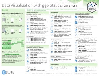
ggplot2 is a grammar of graphics package for creating plots in R. It allows building graphs from data, a coordinate system, and geoms (visual marks). Geoms represent data points and their aesthetic properties like color, size, and position on the plot. Common geoms include points, lines, and bars. Scales map data values to visual properties. Coordinate systems define the space in which geoms are drawn.

1. Data Visualization with ggplot2 : : CHEAT SHEET
ggplot2 is based on the grammar of graphics, the idea
that you can build every graph from the same
components: a data set, a coordinate system,
and geoms—visual marks that represent data points.
Basics
GRAPHICAL PRIMITIVES
a + geom_blank()
(Useful for expanding limits)
b + geom_curve(aes(yend = lat + 1,
xend=long+1),curvature=1) - x, xend, y, yend,
alpha, angle, color, curvature, linetype, size
a + geom_path(lineend="butt", linejoin="round",
linemitre=1)
x, y, alpha, color, group, linetype, size
a + geom_polygon(aes(group = group))
x, y, alpha, color, fill, group, linetype, size
b + geom_rect(aes(xmin = long, ymin=lat, xmax=
long + 1, ymax = lat + 1)) - xmax, xmin, ymax,
ymin, alpha, color, fill, linetype, size
a + geom_ribbon(aes(ymin=unemploy - 900,
ymax=unemploy + 900)) - x, ymax, ymin,
alpha, color, fill, group, linetype, size
+ =
To display values, map variables in the data to visual
properties of the geom (aesthetics) like size, color, and x
and y locations.
+ =
data geom
x = F · y = A
coordinate
system
plot
data geom
x = F · y = A
color = F
size = A
coordinate
system
plot
Complete the template below to build a graph.
required
ggplot(data = mpg, aes(x = cty, y = hwy)) Begins a plot
that you finish by adding layers to. Add one geom
function per layer.
qplot(x = cty, y = hwy, data = mpg, geom = “point")
Creates a complete plot with given data, geom, and
mappings. Supplies many useful defaults.
last_plot() Returns the last plot
ggsave("plot.png", width = 5, height = 5) Saves last plot
as 5’ x 5’ file named "plot.png" in working directory.
Matches file type to file extension.
F M A
F M A
aesthetic mappings data geom
LINE SEGMENTS
b + geom_abline(aes(intercept=0, slope=1))
b + geom_hline(aes(yintercept = lat))
b + geom_vline(aes(xintercept = long))
common aesthetics: x, y, alpha, color, linetype, size
b + geom_segment(aes(yend=lat+1, xend=long+1))
b + geom_spoke(aes(angle = 1:1155, radius = 1))
a <- ggplot(economics, aes(date, unemploy))
b <- ggplot(seals, aes(x = long, y = lat))
ONE VARIABLE continuous
c <- ggplot(mpg, aes(hwy)); c2 <- ggplot(mpg)
c + geom_area(stat = "bin")
x, y, alpha, color, fill, linetype, size
c + geom_density(kernel = "gaussian")
x, y, alpha, color, fill, group, linetype, size, weight
c + geom_dotplot()
x, y, alpha, color, fill
c + geom_freqpoly() x, y, alpha, color, group,
linetype, size
c + geom_histogram(binwidth = 5) x, y, alpha,
color, fill, linetype, size, weight
c2 + geom_qq(aes(sample = hwy)) x, y, alpha,
color, fill, linetype, size, weight
discrete
d <- ggplot(mpg, aes(fl))
d + geom_bar()
x, alpha, color, fill, linetype, size, weight
e + geom_label(aes(label = cty), nudge_x = 1,
nudge_y = 1, check_overlap = TRUE) x, y, label,
alpha, angle, color, family, fontface, hjust,
lineheight, size, vjust
e + geom_jitter(height = 2, width = 2)
x, y, alpha, color, fill, shape, size
e + geom_point(), x, y, alpha, color, fill, shape,
size, stroke
e + geom_quantile(), x, y, alpha, color, group,
linetype, size, weight
e + geom_rug(sides = "bl"), x, y, alpha, color,
linetype, size
e + geom_smooth(method = lm), x, y, alpha,
color, fill, group, linetype, size, weight
e + geom_text(aes(label = cty), nudge_x = 1,
nudge_y = 1, check_overlap = TRUE), x, y, label,
alpha, angle, color, family, fontface, hjust,
lineheight, size, vjust
discrete x , continuous y
f <- ggplot(mpg, aes(class, hwy))
f + geom_col(), x, y, alpha, color, fill, group,
linetype, size
f + geom_boxplot(), x, y, lower, middle, upper,
ymax, ymin, alpha, color, fill, group, linetype,
shape, size, weight
f + geom_dotplot(binaxis = "y", stackdir =
"center"), x, y, alpha, color, fill, group
f + geom_violin(scale = "area"), x, y, alpha, color,
fill, group, linetype, size, weight
discrete x , discrete y
g <- ggplot(diamonds, aes(cut, color))
g + geom_count(), x, y, alpha, color, fill, shape,
size, stroke
THREE VARIABLES
seals$z <- with(seals, sqrt(delta_long^2 + delta_lat^2)); l <- ggplot(seals, aes(long, lat))
l + geom_contour(aes(z = z))
x, y, z, alpha, colour, group, linetype,
size, weight
l + geom_raster(aes(fill = z), hjust=0.5, vjust=0.5,
interpolate=FALSE)
x, y, alpha, fill
l + geom_tile(aes(fill = z)), x, y, alpha, color, fill,
linetype, size, width
h + geom_bin2d(binwidth = c(0.25, 500))
x, y, alpha, color, fill, linetype, size, weight
h + geom_density2d()
x, y, alpha, colour, group, linetype, size
h + geom_hex()
x, y, alpha, colour, fill, size
i + geom_area()
x, y, alpha, color, fill, linetype, size
i + geom_line()
x, y, alpha, color, group, linetype, size
i + geom_step(direction = "hv")
x, y, alpha, color, group, linetype, size
j + geom_crossbar(fatten = 2)
x, y, ymax, ymin, alpha, color, fill, group, linetype,
size
j + geom_errorbar(), x, ymax, ymin, alpha, color,
group, linetype, size, width (also
geom_errorbarh())
j + geom_linerange()
x, ymin, ymax, alpha, color, group, linetype, size
j + geom_pointrange()
x, y, ymin, ymax, alpha, color, fill, group, linetype,
shape, size
continuous function
i <- ggplot(economics, aes(date, unemploy))
visualizing error
df <- data.frame(grp = c("A", "B"), fit = 4:5, se = 1:2)
j <- ggplot(df, aes(grp, fit, ymin = fit-se, ymax = fit+se))
maps
data <- data.frame(murder = USArrests$Murder,
state = tolower(rownames(USArrests)))
map <- map_data("state")
k <- ggplot(data, aes(fill = murder))
k + geom_map(aes(map_id = state), map = map)
+ expand_limits(x = map$long, y = map$lat),
map_id, alpha, color, fill, linetype, size
Not
required,
sensible
defaults
supplied
Geoms Use a geom function to represent data points, use the geom’s aesthetic properties to represent variables.
Each function returns a layer.
TWO VARIABLES
continuous x , continuous y
e <- ggplot(mpg, aes(cty, hwy))
continuous bivariate distribution
h <- ggplot(diamonds, aes(carat, price))
RStudio® is a trademark of RStudio, Inc. • CC BY SA RStudio • info@rstudio.com • 844-448-1212 • rstudio.com • Learn more at http://ggplot2.tidyverse.org • ggplot2 3.1.0 • Updated: 2018-12
ggplot (data = <DATA> ) +
<GEOM_FUNCTION> (mapping = aes( <MAPPINGS> ),
stat = <STAT> , position = <POSITION> ) +
<COORDINATE_FUNCTION> +
<FACET_FUNCTION> +
<SCALE_FUNCTION> +
<THEME_FUNCTION>

2. Scales Coordinate Systems
A stat builds new variables to plot (e.g., count, prop).
Stats An alternative way to build a layer
+ =
data geom
x = x ·
y = ..count..
coordinate
system
plot
fl cty cyl
x ..count..
stat
Visualize a stat by changing the default stat of a geom
function, geom_bar(stat="count") or by using a stat
function, stat_count(geom="bar"), which calls a default
geom to make a layer (equivalent to a geom function).
Use ..name.. syntax to map stat variables to aesthetics.
i + stat_density2d(aes(fill = ..level..),
geom = "polygon")
stat function geommappings
variable created by stat
geom to use
c + stat_bin(binwidth = 1, origin = 10)
x, y | ..count.., ..ncount.., ..density.., ..ndensity..
c + stat_count(width = 1) x, y, | ..count.., ..prop..
c + stat_density(adjust = 1, kernel = “gaussian")
x, y, | ..count.., ..density.., ..scaled..
e + stat_bin_2d(bins = 30, drop = T)
x, y, fill | ..count.., ..density..
e + stat_bin_hex(bins=30) x, y, fill | ..count.., ..density..
e + stat_density_2d(contour = TRUE, n = 100)
x, y, color, size | ..level..
e + stat_ellipse(level = 0.95, segments = 51, type = "t")
l + stat_contour(aes(z = z)) x, y, z, order | ..level..
l + stat_summary_hex(aes(z = z), bins = 30, fun = max)
x, y, z, fill | ..value..
l + stat_summary_2d(aes(z = z), bins = 30, fun = mean)
x, y, z, fill | ..value..
f + stat_boxplot(coef = 1.5) x, y | ..lower..,
..middle.., ..upper.., ..width.. , ..ymin.., ..ymax..
f + stat_ydensity(kernel = "gaussian", scale = “area") x, y |
..density.., ..scaled.., ..count.., ..n.., ..violinwidth.., ..width..
e + stat_ecdf(n = 40) x, y | ..x.., ..y..
e + stat_quantile(quantiles = c(0.1, 0.9), formula = y ~
log(x), method = "rq") x, y | ..quantile..
e + stat_smooth(method = "lm", formula = y ~ x, se=T,
level=0.95) x, y | ..se.., ..x.., ..y.., ..ymin.., ..ymax..
ggplot() + stat_function(aes(x = -3:3), n = 99, fun =
dnorm, args = list(sd=0.5)) x | ..x.., ..y..
e + stat_identity(na.rm = TRUE)
ggplot() + stat_qq(aes(sample=1:100), dist = qt,
dparam=list(df=5)) sample, x, y | ..sample.., ..theoretical..
e + stat_sum() x, y, size | ..n.., ..prop..
e + stat_summary(fun.data = "mean_cl_boot")
h + stat_summary_bin(fun = "mean", geom = "bar")
e + stat_unique()
Scales map data values to the visual values of an
aesthetic. To change a mapping, add a new scale.
(n <- d + geom_bar(aes(fill = fl)))
n + scale_fill_manual(
values = c("skyblue", "royalblue", "blue", “navy"),
limits = c("d", "e", "p", "r"), breaks =c("d", "e", "p", “r"),
name = "fuel", labels = c("D", "E", "P", "R"))
scale_
aesthetic
to adjust
prepackaged
scale to use
scale-specific
arguments
title to use in
legend/axis
labels to use
in legend/axis
breaks to use in
legend/axis
range of
values to include
in mapping
GENERAL PURPOSE SCALES
Use with most aesthetics
scale_*_continuous() - map cont’ values to visual ones
scale_*_discrete() - map discrete values to visual ones
scale_*_identity() - use data values as visual ones
scale_*_manual(values = c()) - map discrete values to
manually chosen visual ones
scale_*_date(date_labels = "%m/%d"), date_breaks = "2
weeks") - treat data values as dates.
scale_*_datetime() - treat data x values as date times.
Use same arguments as scale_x_date(). See ?strptime for
label formats.
X & Y LOCATION SCALES
Use with x or y aesthetics (x shown here)
scale_x_log10() - Plot x on log10 scale
scale_x_reverse() - Reverse direction of x axis
scale_x_sqrt() - Plot x on square root scale
COLOR AND FILL SCALES (DISCRETE)
n <- d + geom_bar(aes(fill = fl))
n + scale_fill_brewer(palette = "Blues")
For palette choices:
RColorBrewer::display.brewer.all()
n + scale_fill_grey(start = 0.2, end = 0.8,
na.value = "red")
COLOR AND FILL SCALES (CONTINUOUS)
o <- c + geom_dotplot(aes(fill = ..x..))
o + scale_fill_distiller(palette = "Blues")
o + scale_fill_gradient(low="red", high="yellow")
o + scale_fill_gradient2(low="red", high=“blue",
mid = "white", midpoint = 25)
o + scale_fill_gradientn(colours=topo.colors(6))
Also: rainbow(), heat.colors(), terrain.colors(),
cm.colors(), RColorBrewer::brewer.pal()
SHAPE AND SIZE SCALES
p <- e + geom_point(aes(shape = fl, size = cyl))
p + scale_shape() + scale_size()
p + scale_shape_manual(values = c(3:7))
p + scale_radius(range = c(1,6))
p + scale_size_area(max_size = 6)
r <- d + geom_bar()
r + coord_cartesian(xlim = c(0, 5))
xlim, ylim
The default cartesian coordinate system
r + coord_fixed(ratio = 1/2)
ratio, xlim, ylim
Cartesian coordinates with fixed aspect ratio
between x and y units
r + coord_flip()
xlim, ylim
Flipped Cartesian coordinates
r + coord_polar(theta = "x", direction=1 )
theta, start, direction
Polar coordinates
r + coord_trans(ytrans = “sqrt")
xtrans, ytrans, limx, limy
Transformed cartesian coordinates. Set xtrans and
ytrans to the name of a window function.
π + coord_quickmap()
π + coord_map(projection = "ortho",
orientation=c(41, -74, 0))projection, xlim, ylim
Map projections from the mapproj package
(mercator (default), azequalarea, lagrange, etc.)
Position Adjustments
Position adjustments determine how to arrange geoms
that would otherwise occupy the same space.
s <- ggplot(mpg, aes(fl, fill = drv))
s + geom_bar(position = "dodge")
Arrange elements side by side
s + geom_bar(position = "fill")
Stack elements on top of one another,
normalize height
e + geom_point(position = "jitter")
Add random noise to X and Y position of each
element to avoid overplotting
e + geom_label(position = "nudge")
Nudge labels away from points
s + geom_bar(position = "stack")
Stack elements on top of one another
Each position adjustment can be recast as a function with
manual width and height arguments
s + geom_bar(position = position_dodge(width = 1))
A
B
Themes
r + theme_bw()
White background
with grid lines
r + theme_gray()
Grey background
(default theme)
r + theme_dark()
dark for contrast
r + theme_classic()
r + theme_light()
r + theme_linedraw()
r + theme_minimal()
Minimal themes
r + theme_void()
Empty theme
Faceting
Facets divide a plot into
subplots based on the
values of one or more
discrete variables.
t <- ggplot(mpg, aes(cty, hwy)) + geom_point()
t + facet_grid(cols = vars(fl))
facet into columns based on fl
t + facet_grid(rows = vars(year))
facet into rows based on year
t + facet_grid(rows = vars(year), cols = vars(fl))
facet into both rows and columns
t + facet_wrap(vars(fl))
wrap facets into a rectangular layout
Set scales to let axis limits vary across facets
t + facet_grid(rows = vars(drv), cols = vars(fl),
scales = "free")
x and y axis limits adjust to individual facets
"free_x" - x axis limits adjust
"free_y" - y axis limits adjust
Set labeller to adjust facet labels
t + facet_grid(cols = vars(fl), labeller = label_both)
t + facet_grid(rows = vars(fl),
labeller = label_bquote(alpha ^ .(fl)))
fl: c fl: d fl: e fl: p fl: r
↵c
↵d ↵e
↵p
↵r
Labels
t + labs( x = "New x axis label", y = "New y axis label",
title ="Add a title above the plot",
subtitle = "Add a subtitle below title",
caption = "Add a caption below plot",
<aes> = "New <aes> legend title")
t + annotate(geom = "text", x = 8, y = 9, label = "A")
Use scale functions
to update legend
labels
<AES>
geom to place manual values for geom’s aesthetics
<AES>
Legends
n + theme(legend.position = "bottom")
Place legend at "bottom", "top", "le
ft
", or "right"
n + guides(fill = "none")
Set legend type for each aesthetic: colorbar, legend, or
none (no legend)
n + scale_fill_discrete(name = "Title",
labels = c("A", "B", "C", "D", "E"))
Set legend title and labels with a scale function.
Zooming
Without clipping (preferred)
t + coord_cartesian(
xlim = c(0, 100), ylim = c(10, 20))
With clipping (removes unseen data points)
t + xlim(0, 100) + ylim(10, 20)
t + scale_x_continuous(limits = c(0, 100)) +
scale_y_continuous(limits = c(0, 100))
RStudio® is a trademark of RStudio, Inc. • CC BY SA RStudio • info@rstudio.com • 844-448-1212 • rstudio.com • Learn more at http://ggplot2.tidyverse.org • ggplot2 3.1.0 • Updated: 2018-12
60
long
lat