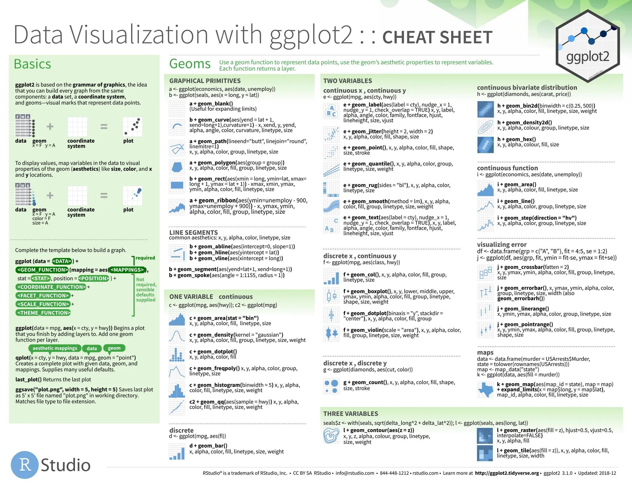
Data Visualization with ggplot2 : : CHEAT SHEET
ggplot2 is based on the grammar of graphics, the idea
that you can build every graph from the same
components: a data set, a coordinate system,
and geoms—visual marks that represent data points.
Basics
GRAPHICAL PRIMITIVES
a + geom_blank()
(Useful for expanding limits)
b + geom_curve(aes(yend = lat + 1,
xend=long+1),curvature=1) - x, xend, y, yend,
alpha, angle, color, curvature, linetype, size
a + geom_path(lineend="butt", linejoin="round",
linemitre=1)
x, y, alpha, color, group, linetype, size
a + geom_polygon(aes(group = group))
x, y, alpha, color, fill, group, linetype, size
b + geom_rect(aes(xmin = long, ymin=lat, xmax=
long + 1, ymax = lat + 1)) - xmax, xmin, ymax,
ymin, alpha, color, fill, linetype, size
a + geom_ribbon(aes(ymin=unemploy - 900,
ymax=unemploy + 900)) - x, ymax, ymin,
alpha, color, fill, group, linetype, size
+ =
To display values, map variables in the data to visual
properties of the geom (aesthetics) like size, color, and x
and y locations.
+ =
data geom
x = F · y = A
coordinate
system
plot
data geom
x = F · y = A
color = F
size = A
coordinate
system
plot
Complete the template below to build a graph.
required
ggplot(data = mpg, aes(x = cty, y = hwy)) Begins a plot
that you finish by adding layers to. Add one geom
function per layer.
qplot(x = cty, y = hwy, data = mpg, geom = “point")
Creates a complete plot with given data, geom, and
mappings. Supplies many useful defaults.
last_plot() Returns the last plot
ggsave("plot.png", width = 5, height = 5) Saves last plot
as 5’ x 5’ file named "plot.png" in working directory.
Matches file type to file extension.
F M A
F M A
aesthetic mappings data geom
LINE SEGMENTS
b + geom_abline(aes(intercept=0, slope=1))
b + geom_hline(aes(yintercept = lat))
b + geom_vline(aes(xintercept = long))
common aesthetics: x, y, alpha, color, linetype, size
b + geom_segment(aes(yend=lat+1, xend=long+1))
b + geom_spoke(aes(angle = 1:1155, radius = 1))
a <- ggplot(economics, aes(date, unemploy))
b <- ggplot(seals, aes(x = long, y = lat))
ONE VARIABLE continuous
c <- ggplot(mpg, aes(hwy)); c2 <- ggplot(mpg)
c + geom_area(stat = "bin")
x, y, alpha, color, fill, linetype, size
c + geom_density(kernel = "gaussian")
x, y, alpha, color, fill, group, linetype, size, weight
c + geom_dotplot()
x, y, alpha, color, fill
c + geom_freqpoly() x, y, alpha, color, group,
linetype, size
c + geom_histogram(binwidth = 5) x, y, alpha,
color, fill, linetype, size, weight
c2 + geom_qq(aes(sample = hwy)) x, y, alpha,
color, fill, linetype, size, weight
discrete
d <- ggplot(mpg, aes(fl))
d + geom_bar()
x, alpha, color, fill, linetype, size, weight
e + geom_label(aes(label = cty), nudge_x = 1,
nudge_y = 1, check_overlap = TRUE) x, y, label,
alpha, angle, color, family, fontface, hjust,
lineheight, size, vjust
e + geom_jitter(height = 2, width = 2)
x, y, alpha, color, fill, shape, size
e + geom_point(), x, y, alpha, color, fill, shape,
size, stroke
e + geom_quantile(), x, y, alpha, color, group,
linetype, size, weight
e + geom_rug(sides = "bl"), x, y, alpha, color,
linetype, size
e + geom_smooth(method = lm), x, y, alpha,
color, fill, group, linetype, size, weight
e + geom_text(aes(label = cty), nudge_x = 1,
nudge_y = 1, check_overlap = TRUE), x, y, label,
alpha, angle, color, family, fontface, hjust,
lineheight, size, vjust
discrete x , continuous y
f <- ggplot(mpg, aes(class, hwy))
f + geom_col(), x, y, alpha, color, fill, group,
linetype, size
f + geom_boxplot(), x, y, lower, middle, upper,
ymax, ymin, alpha, color, fill, group, linetype,
shape, size, weight
f + geom_dotplot(binaxis = "y", stackdir =
"center"), x, y, alpha, color, fill, group
f + geom_violin(scale = "area"), x, y, alpha, color,
fill, group, linetype, size, weight
discrete x , discrete y
g <- ggplot(diamonds, aes(cut, color))
g + geom_count(), x, y, alpha, color, fill, shape,
size, stroke
THREE VARIABLES
seals$z <- with(seals, sqrt(delta_long^2 + delta_lat^2)); l <- ggplot(seals, aes(long, lat))
l + geom_contour(aes(z = z))
x, y, z, alpha, colour, group, linetype,
size, weight
l + geom_raster(aes(fill = z), hjust=0.5, vjust=0.5,
interpolate=FALSE)
x, y, alpha, fill
l + geom_tile(aes(fill = z)), x, y, alpha, color, fill,
linetype, size, width
h + geom_bin2d(binwidth = c(0.25, 500))
x, y, alpha, color, fill, linetype, size, weight
h + geom_density2d()
x, y, alpha, colour, group, linetype, size
h + geom_hex()
x, y, alpha, colour, fill, size
i + geom_area()
x, y, alpha, color, fill, linetype, size
i + geom_line()
x, y, alpha, color, group, linetype, size
i + geom_step(direction = "hv")
x, y, alpha, color, group, linetype, size
j + geom_crossbar(fatten = 2)
x, y, ymax, ymin, alpha, color, fill, group, linetype,
size
j + geom_errorbar(), x, ymax, ymin, alpha, color,
group, linetype, size, width (also
geom_errorbarh())
j + geom_linerange()
x, ymin, ymax, alpha, color, group, linetype, size
j + geom_pointrange()
x, y, ymin, ymax, alpha, color, fill, group, linetype,
shape, size
continuous function
i <- ggplot(economics, aes(date, unemploy))
visualizing error
df <- data.frame(grp = c("A", "B"), fit = 4:5, se = 1:2)
j <- ggplot(df, aes(grp, fit, ymin = fit-se, ymax = fit+se))
maps
data <- data.frame(murder = USArrests$Murder,
state = tolower(rownames(USArrests)))
map <- map_data("state")
k <- ggplot(data, aes(fill = murder))
k + geom_map(aes(map_id = state), map = map)
+ expand_limits(x = map$long, y = map$lat),
map_id, alpha, color, fill, linetype, size
Not
required,
sensible
defaults
supplied
Geoms Use a geom function to represent data points, use the geom’s aesthetic properties to represent variables.
Each function returns a layer.
TWO VARIABLES
continuous x , continuous y
e <- ggplot(mpg, aes(cty, hwy))
continuous bivariate distribution
h <- ggplot(diamonds, aes(carat, price))
RStudio® is a trademark of RStudio, Inc. • CC BY SA RStudio • info@rstudio.com • 844-448-1212 • rstudio.com • Learn more at http://ggplot2.tidyverse.org • ggplot2 3.1.0 • Updated: 2018-12
ggplot (data = <DATA> ) +
<GEOM_FUNCTION> (mapping = aes( <MAPPINGS> ),
stat = <STAT> , position = <POSITION> ) +
<COORDINATE_FUNCTION> +
<FACET_FUNCTION> +
<SCALE_FUNCTION> +
<THEME_FUNCTION>
Scales Coordinate Systems
A stat builds new variables to plot (e.g., count, prop).
Stats An alternative way to build a layer
+ =
data geom
x = x ·
y = ..count..
coordinate
system
plot
fl cty cyl
x ..count..
stat
Visualize a stat by changing the default stat of a geom
function, geom_bar(stat="count") or by using a stat
function, stat_count(geom="bar"), which calls a default
geom to make a layer (equivalent to a geom function).
Use ..name.. syntax to map stat variables to aesthetics.
i + stat_density2d(aes(fill = ..level..),
geom = "polygon")
stat function geommappings
variable created by stat
geom to use
c + stat_bin(binwidth = 1, origin = 10)
x, y | ..count.., ..ncount.., ..density.., ..ndensity..
c + stat_count(width = 1) x, y, | ..count.., ..prop..
c + stat_density(adjust = 1, kernel = “gaussian")
x, y, | ..count.., ..density.., ..scaled..
e + stat_bin_2d(bins = 30, drop = T)
x, y, fill | ..count.., ..density..
e + stat_bin_hex(bins=30) x, y, fill | ..count.., ..density..
e + stat_density_2d(contour = TRUE, n = 100)
x, y, color, size | ..level..
e + stat_ellipse(level = 0.95, segments = 51, type = "t")
l + stat_contour(aes(z = z)) x, y, z, order | ..level..
l + stat_summary_hex(aes(z = z), bins = 30, fun = max)
x, y, z, fill | ..value..
l + stat_summary_2d(aes(z = z), bins = 30, fun = mean)
x, y, z, fill | ..value..
f + stat_boxplot(coef = 1.5) x, y | ..lower..,
..middle.., ..upper.., ..width.. , ..ymin.., ..ymax..
f + stat_ydensity(kernel = "gaussian", scale = “area") x, y |
..density.., ..scaled.., ..count.., ..n.., ..violinwidth.., ..width..
e + stat_ecdf(n = 40) x, y | ..x.., ..y..
e + stat_quantile(quantiles = c(0.1, 0.9), formula = y ~
log(x), method = "rq") x, y | ..quantile..
e + stat_smooth(method = "lm", formula = y ~ x, se=T,
level=0.95) x, y | ..se.., ..x.., ..y.., ..ymin.., ..ymax..
ggplot() + stat_function(aes(x = -3:3), n = 99, fun =
dnorm, args = list(sd=0.5)) x | ..x.., ..y..
e + stat_identity(na.rm = TRUE)
ggplot() + stat_qq(aes(sample=1:100), dist = qt,
dparam=list(df=5)) sample, x, y | ..sample.., ..theoretical..
e + stat_sum() x, y, size | ..n.., ..prop..
e + stat_summary(fun.data = "mean_cl_boot")
h + stat_summary_bin(fun = "mean", geom = "bar")
e + stat_unique()
Scales map data values to the visual values of an
aesthetic. To change a mapping, add a new scale.
(n <- d + geom_bar(aes(fill = fl)))
n + scale_fill_manual(
values = c("skyblue", "royalblue", "blue", “navy"),
limits = c("d", "e", "p", "r"), breaks =c("d", "e", "p", “r"),
name = "fuel", labels = c("D", "E", "P", "R"))
scale_
aesthetic
to adjust
prepackaged
scale to use
scale-specific
arguments
title to use in
legend/axis
labels to use
in legend/axis
breaks to use in
legend/axis
range of
values to include
in mapping
GENERAL PURPOSE SCALES
Use with most aesthetics
scale_*_continuous() - map cont’ values to visual ones
scale_*_discrete() - map discrete values to visual ones
scale_*_identity() - use data values as visual ones
scale_*_manual(values = c()) - map discrete values to
manually chosen visual ones
scale_*_date(date_labels = "%m/%d"), date_breaks = "2
weeks") - treat data values as dates.
scale_*_datetime() - treat data x values as date times.
Use same arguments as scale_x_date(). See ?strptime for
label formats.
X & Y LOCATION SCALES
Use with x or y aesthetics (x shown here)
scale_x_log10() - Plot x on log10 scale
scale_x_reverse() - Reverse direction of x axis
scale_x_sqrt() - Plot x on square root scale
COLOR AND FILL SCALES (DISCRETE)
n <- d + geom_bar(aes(fill = fl))
n + scale_fill_brewer(palette = "Blues")
For palette choices:
RColorBrewer::display.brewer.all()
n + scale_fill_grey(start = 0.2, end = 0.8,
na.value = "red")
COLOR AND FILL SCALES (CONTINUOUS)
o <- c + geom_dotplot(aes(fill = ..x..))
o + scale_fill_distiller(palette = "Blues")
o + scale_fill_gradient(low="red", high="yellow")
o + scale_fill_gradient2(low="red", high=“blue",
mid = "white", midpoint = 25)
o + scale_fill_gradientn(colours=topo.colors(6))
Also: rainbow(), heat.colors(), terrain.colors(),
cm.colors(), RColorBrewer::brewer.pal()
SHAPE AND SIZE SCALES
p <- e + geom_point(aes(shape = fl, size = cyl))
p + scale_shape() + scale_size()
p + scale_shape_manual(values = c(3:7))
p + scale_radius(range = c(1,6))
p + scale_size_area(max_size = 6)
r <- d + geom_bar()
r + coord_cartesian(xlim = c(0, 5))
xlim, ylim
The default cartesian coordinate system
r + coord_fixed(ratio = 1/2)
ratio, xlim, ylim
Cartesian coordinates with fixed aspect ratio
between x and y units
r + coord_flip()
xlim, ylim
Flipped Cartesian coordinates
r + coord_polar(theta = "x", direction=1 )
theta, start, direction
Polar coordinates
r + coord_trans(ytrans = “sqrt")
xtrans, ytrans, limx, limy
Transformed cartesian coordinates. Set xtrans and
ytrans to the name of a window function.
π + coord_quickmap()
π + coord_map(projection = "ortho",
orientation=c(41, -74, 0))projection, xlim, ylim
Map projections from the mapproj package
(mercator (default), azequalarea, lagrange, etc.)
Position Adjustments
Position adjustments determine how to arrange geoms
that would otherwise occupy the same space.
s <- ggplot(mpg, aes(fl, fill = drv))
s + geom_bar(position = "dodge")
Arrange elements side by side
s + geom_bar(position = "fill")
Stack elements on top of one another,
normalize height
e + geom_point(position = "jitter")
Add random noise to X and Y position of each
element to avoid overplotting
e + geom_label(position = "nudge")
Nudge labels away from points
s + geom_bar(position = "stack")
Stack elements on top of one another
Each position adjustment can be recast as a function with
manual width and height arguments
s + geom_bar(position = position_dodge(width = 1))
A
B
Themes
r + theme_bw()
White background
with grid lines
r + theme_gray()
Grey background
(default theme)
r + theme_dark()
dark for contrast
r + theme_classic()
r + theme_light()
r + theme_linedraw()
r + theme_minimal()
Minimal themes
r + theme_void()
Empty theme
Faceting
Facets divide a plot into
subplots based on the
values of one or more
discrete variables.
t <- ggplot(mpg, aes(cty, hwy)) + geom_point()
t + facet_grid(cols = vars(fl))
facet into columns based on fl
t + facet_grid(rows = vars(year))
facet into rows based on year
t + facet_grid(rows = vars(year), cols = vars(fl))
facet into both rows and columns
t + facet_wrap(vars(fl))
wrap facets into a rectangular layout
Set scales to let axis limits vary across facets
t + facet_grid(rows = vars(drv), cols = vars(fl),
scales = "free")
x and y axis limits adjust to individual facets
"free_x" - x axis limits adjust
"free_y" - y axis limits adjust
Set labeller to adjust facet labels
t + facet_grid(cols = vars(fl), labeller = label_both)
t + facet_grid(rows = vars(fl),
labeller = label_bquote(alpha ^ .(fl)))
fl: c fl: d fl: e fl: p fl: r
↵c
↵d ↵e
↵p
↵r
Labels
t + labs( x = "New x axis label", y = "New y axis label",
title ="Add a title above the plot",
subtitle = "Add a subtitle below title",
caption = "Add a caption below plot",
<aes> = "New <aes> legend title")
t + annotate(geom = "text", x = 8, y = 9, label = "A")
Use scale functions
to update legend
labels
<AES>
geom to place manual values for geom’s aesthetics
<AES>
Legends
n + theme(legend.position = "bottom")
Place legend at "bottom", "top", "le
ft
", or "right"
n + guides(fill = "none")
Set legend type for each aesthetic: colorbar, legend, or
none (no legend)
n + scale_fill_discrete(name = "Title",
labels = c("A", "B", "C", "D", "E"))
Set legend title and labels with a scale function.
Zooming
Without clipping (preferred)
t + coord_cartesian(
xlim = c(0, 100), ylim = c(10, 20))
With clipping (removes unseen data points)
t + xlim(0, 100) + ylim(10, 20)
t + scale_x_continuous(limits = c(0, 100)) +
scale_y_continuous(limits = c(0, 100))
RStudio® is a trademark of RStudio, Inc. • CC BY SA RStudio • info@rstudio.com • 844-448-1212 • rstudio.com • Learn more at http://ggplot2.tidyverse.org • ggplot2 3.1.0 • Updated: 2018-12
60
long
lat

Data Visualization with ggplot2.pdf

  • 1.
    Data Visualization withggplot2 : : CHEAT SHEET ggplot2 is based on the grammar of graphics, the idea that you can build every graph from the same components: a data set, a coordinate system, and geoms—visual marks that represent data points. Basics GRAPHICAL PRIMITIVES a + geom_blank() (Useful for expanding limits) b + geom_curve(aes(yend = lat + 1, xend=long+1),curvature=1) - x, xend, y, yend, alpha, angle, color, curvature, linetype, size a + geom_path(lineend="butt", linejoin="round", linemitre=1) x, y, alpha, color, group, linetype, size a + geom_polygon(aes(group = group)) x, y, alpha, color, fill, group, linetype, size b + geom_rect(aes(xmin = long, ymin=lat, xmax= long + 1, ymax = lat + 1)) - xmax, xmin, ymax, ymin, alpha, color, fill, linetype, size a + geom_ribbon(aes(ymin=unemploy - 900, ymax=unemploy + 900)) - x, ymax, ymin, alpha, color, fill, group, linetype, size + = To display values, map variables in the data to visual properties of the geom (aesthetics) like size, color, and x and y locations. + = data geom x = F · y = A coordinate system plot data geom x = F · y = A color = F size = A coordinate system plot Complete the template below to build a graph. required ggplot(data = mpg, aes(x = cty, y = hwy)) Begins a plot that you finish by adding layers to. Add one geom function per layer. qplot(x = cty, y = hwy, data = mpg, geom = “point") Creates a complete plot with given data, geom, and mappings. Supplies many useful defaults. last_plot() Returns the last plot ggsave("plot.png", width = 5, height = 5) Saves last plot as 5’ x 5’ file named "plot.png" in working directory. Matches file type to file extension. F M A F M A aesthetic mappings data geom LINE SEGMENTS b + geom_abline(aes(intercept=0, slope=1)) b + geom_hline(aes(yintercept = lat)) b + geom_vline(aes(xintercept = long)) common aesthetics: x, y, alpha, color, linetype, size b + geom_segment(aes(yend=lat+1, xend=long+1)) b + geom_spoke(aes(angle = 1:1155, radius = 1)) a <- ggplot(economics, aes(date, unemploy)) b <- ggplot(seals, aes(x = long, y = lat)) ONE VARIABLE continuous c <- ggplot(mpg, aes(hwy)); c2 <- ggplot(mpg) c + geom_area(stat = "bin") x, y, alpha, color, fill, linetype, size c + geom_density(kernel = "gaussian") x, y, alpha, color, fill, group, linetype, size, weight c + geom_dotplot() x, y, alpha, color, fill c + geom_freqpoly() x, y, alpha, color, group, linetype, size c + geom_histogram(binwidth = 5) x, y, alpha, color, fill, linetype, size, weight c2 + geom_qq(aes(sample = hwy)) x, y, alpha, color, fill, linetype, size, weight discrete d <- ggplot(mpg, aes(fl)) d + geom_bar() x, alpha, color, fill, linetype, size, weight e + geom_label(aes(label = cty), nudge_x = 1, nudge_y = 1, check_overlap = TRUE) x, y, label, alpha, angle, color, family, fontface, hjust, lineheight, size, vjust e + geom_jitter(height = 2, width = 2) x, y, alpha, color, fill, shape, size e + geom_point(), x, y, alpha, color, fill, shape, size, stroke e + geom_quantile(), x, y, alpha, color, group, linetype, size, weight e + geom_rug(sides = "bl"), x, y, alpha, color, linetype, size e + geom_smooth(method = lm), x, y, alpha, color, fill, group, linetype, size, weight e + geom_text(aes(label = cty), nudge_x = 1, nudge_y = 1, check_overlap = TRUE), x, y, label, alpha, angle, color, family, fontface, hjust, lineheight, size, vjust discrete x , continuous y f <- ggplot(mpg, aes(class, hwy)) f + geom_col(), x, y, alpha, color, fill, group, linetype, size f + geom_boxplot(), x, y, lower, middle, upper, ymax, ymin, alpha, color, fill, group, linetype, shape, size, weight f + geom_dotplot(binaxis = "y", stackdir = "center"), x, y, alpha, color, fill, group f + geom_violin(scale = "area"), x, y, alpha, color, fill, group, linetype, size, weight discrete x , discrete y g <- ggplot(diamonds, aes(cut, color)) g + geom_count(), x, y, alpha, color, fill, shape, size, stroke THREE VARIABLES seals$z <- with(seals, sqrt(delta_long^2 + delta_lat^2)); l <- ggplot(seals, aes(long, lat)) l + geom_contour(aes(z = z)) x, y, z, alpha, colour, group, linetype, size, weight l + geom_raster(aes(fill = z), hjust=0.5, vjust=0.5, interpolate=FALSE) x, y, alpha, fill l + geom_tile(aes(fill = z)), x, y, alpha, color, fill, linetype, size, width h + geom_bin2d(binwidth = c(0.25, 500)) x, y, alpha, color, fill, linetype, size, weight h + geom_density2d() x, y, alpha, colour, group, linetype, size h + geom_hex() x, y, alpha, colour, fill, size i + geom_area() x, y, alpha, color, fill, linetype, size i + geom_line() x, y, alpha, color, group, linetype, size i + geom_step(direction = "hv") x, y, alpha, color, group, linetype, size j + geom_crossbar(fatten = 2) x, y, ymax, ymin, alpha, color, fill, group, linetype, size j + geom_errorbar(), x, ymax, ymin, alpha, color, group, linetype, size, width (also geom_errorbarh()) j + geom_linerange() x, ymin, ymax, alpha, color, group, linetype, size j + geom_pointrange() x, y, ymin, ymax, alpha, color, fill, group, linetype, shape, size continuous function i <- ggplot(economics, aes(date, unemploy)) visualizing error df <- data.frame(grp = c("A", "B"), fit = 4:5, se = 1:2) j <- ggplot(df, aes(grp, fit, ymin = fit-se, ymax = fit+se)) maps data <- data.frame(murder = USArrests$Murder, state = tolower(rownames(USArrests))) map <- map_data("state") k <- ggplot(data, aes(fill = murder)) k + geom_map(aes(map_id = state), map = map) + expand_limits(x = map$long, y = map$lat), map_id, alpha, color, fill, linetype, size Not required, sensible defaults supplied Geoms Use a geom function to represent data points, use the geom’s aesthetic properties to represent variables. Each function returns a layer. TWO VARIABLES continuous x , continuous y e <- ggplot(mpg, aes(cty, hwy)) continuous bivariate distribution h <- ggplot(diamonds, aes(carat, price)) RStudio® is a trademark of RStudio, Inc. • CC BY SA RStudio • info@rstudio.com • 844-448-1212 • rstudio.com • Learn more at http://ggplot2.tidyverse.org • ggplot2 3.1.0 • Updated: 2018-12 ggplot (data = <DATA> ) + <GEOM_FUNCTION> (mapping = aes( <MAPPINGS> ), stat = <STAT> , position = <POSITION> ) + <COORDINATE_FUNCTION> + <FACET_FUNCTION> + <SCALE_FUNCTION> + <THEME_FUNCTION>
  • 2.
    Scales Coordinate Systems Astat builds new variables to plot (e.g., count, prop). Stats An alternative way to build a layer + = data geom x = x · y = ..count.. coordinate system plot fl cty cyl x ..count.. stat Visualize a stat by changing the default stat of a geom function, geom_bar(stat="count") or by using a stat function, stat_count(geom="bar"), which calls a default geom to make a layer (equivalent to a geom function). Use ..name.. syntax to map stat variables to aesthetics. i + stat_density2d(aes(fill = ..level..), geom = "polygon") stat function geommappings variable created by stat geom to use c + stat_bin(binwidth = 1, origin = 10) x, y | ..count.., ..ncount.., ..density.., ..ndensity.. c + stat_count(width = 1) x, y, | ..count.., ..prop.. c + stat_density(adjust = 1, kernel = “gaussian") x, y, | ..count.., ..density.., ..scaled.. e + stat_bin_2d(bins = 30, drop = T) x, y, fill | ..count.., ..density.. e + stat_bin_hex(bins=30) x, y, fill | ..count.., ..density.. e + stat_density_2d(contour = TRUE, n = 100) x, y, color, size | ..level.. e + stat_ellipse(level = 0.95, segments = 51, type = "t") l + stat_contour(aes(z = z)) x, y, z, order | ..level.. l + stat_summary_hex(aes(z = z), bins = 30, fun = max) x, y, z, fill | ..value.. l + stat_summary_2d(aes(z = z), bins = 30, fun = mean) x, y, z, fill | ..value.. f + stat_boxplot(coef = 1.5) x, y | ..lower.., ..middle.., ..upper.., ..width.. , ..ymin.., ..ymax.. f + stat_ydensity(kernel = "gaussian", scale = “area") x, y | ..density.., ..scaled.., ..count.., ..n.., ..violinwidth.., ..width.. e + stat_ecdf(n = 40) x, y | ..x.., ..y.. e + stat_quantile(quantiles = c(0.1, 0.9), formula = y ~ log(x), method = "rq") x, y | ..quantile.. e + stat_smooth(method = "lm", formula = y ~ x, se=T, level=0.95) x, y | ..se.., ..x.., ..y.., ..ymin.., ..ymax.. ggplot() + stat_function(aes(x = -3:3), n = 99, fun = dnorm, args = list(sd=0.5)) x | ..x.., ..y.. e + stat_identity(na.rm = TRUE) ggplot() + stat_qq(aes(sample=1:100), dist = qt, dparam=list(df=5)) sample, x, y | ..sample.., ..theoretical.. e + stat_sum() x, y, size | ..n.., ..prop.. e + stat_summary(fun.data = "mean_cl_boot") h + stat_summary_bin(fun = "mean", geom = "bar") e + stat_unique() Scales map data values to the visual values of an aesthetic. To change a mapping, add a new scale. (n <- d + geom_bar(aes(fill = fl))) n + scale_fill_manual( values = c("skyblue", "royalblue", "blue", “navy"), limits = c("d", "e", "p", "r"), breaks =c("d", "e", "p", “r"), name = "fuel", labels = c("D", "E", "P", "R")) scale_ aesthetic to adjust prepackaged scale to use scale-specific arguments title to use in legend/axis labels to use in legend/axis breaks to use in legend/axis range of values to include in mapping GENERAL PURPOSE SCALES Use with most aesthetics scale_*_continuous() - map cont’ values to visual ones scale_*_discrete() - map discrete values to visual ones scale_*_identity() - use data values as visual ones scale_*_manual(values = c()) - map discrete values to manually chosen visual ones scale_*_date(date_labels = "%m/%d"), date_breaks = "2 weeks") - treat data values as dates. scale_*_datetime() - treat data x values as date times. Use same arguments as scale_x_date(). See ?strptime for label formats. X & Y LOCATION SCALES Use with x or y aesthetics (x shown here) scale_x_log10() - Plot x on log10 scale scale_x_reverse() - Reverse direction of x axis scale_x_sqrt() - Plot x on square root scale COLOR AND FILL SCALES (DISCRETE) n <- d + geom_bar(aes(fill = fl)) n + scale_fill_brewer(palette = "Blues") For palette choices: RColorBrewer::display.brewer.all() n + scale_fill_grey(start = 0.2, end = 0.8, na.value = "red") COLOR AND FILL SCALES (CONTINUOUS) o <- c + geom_dotplot(aes(fill = ..x..)) o + scale_fill_distiller(palette = "Blues") o + scale_fill_gradient(low="red", high="yellow") o + scale_fill_gradient2(low="red", high=“blue", mid = "white", midpoint = 25) o + scale_fill_gradientn(colours=topo.colors(6)) Also: rainbow(), heat.colors(), terrain.colors(), cm.colors(), RColorBrewer::brewer.pal() SHAPE AND SIZE SCALES p <- e + geom_point(aes(shape = fl, size = cyl)) p + scale_shape() + scale_size() p + scale_shape_manual(values = c(3:7)) p + scale_radius(range = c(1,6)) p + scale_size_area(max_size = 6) r <- d + geom_bar() r + coord_cartesian(xlim = c(0, 5)) xlim, ylim The default cartesian coordinate system r + coord_fixed(ratio = 1/2) ratio, xlim, ylim Cartesian coordinates with fixed aspect ratio between x and y units r + coord_flip() xlim, ylim Flipped Cartesian coordinates r + coord_polar(theta = "x", direction=1 ) theta, start, direction Polar coordinates r + coord_trans(ytrans = “sqrt") xtrans, ytrans, limx, limy Transformed cartesian coordinates. Set xtrans and ytrans to the name of a window function. π + coord_quickmap() π + coord_map(projection = "ortho", orientation=c(41, -74, 0))projection, xlim, ylim Map projections from the mapproj package (mercator (default), azequalarea, lagrange, etc.) Position Adjustments Position adjustments determine how to arrange geoms that would otherwise occupy the same space. s <- ggplot(mpg, aes(fl, fill = drv)) s + geom_bar(position = "dodge") Arrange elements side by side s + geom_bar(position = "fill") Stack elements on top of one another, normalize height e + geom_point(position = "jitter") Add random noise to X and Y position of each element to avoid overplotting e + geom_label(position = "nudge") Nudge labels away from points s + geom_bar(position = "stack") Stack elements on top of one another Each position adjustment can be recast as a function with manual width and height arguments s + geom_bar(position = position_dodge(width = 1)) A B Themes r + theme_bw() White background with grid lines r + theme_gray() Grey background (default theme) r + theme_dark() dark for contrast r + theme_classic() r + theme_light() r + theme_linedraw() r + theme_minimal() Minimal themes r + theme_void() Empty theme Faceting Facets divide a plot into subplots based on the values of one or more discrete variables. t <- ggplot(mpg, aes(cty, hwy)) + geom_point() t + facet_grid(cols = vars(fl)) facet into columns based on fl t + facet_grid(rows = vars(year)) facet into rows based on year t + facet_grid(rows = vars(year), cols = vars(fl)) facet into both rows and columns t + facet_wrap(vars(fl)) wrap facets into a rectangular layout Set scales to let axis limits vary across facets t + facet_grid(rows = vars(drv), cols = vars(fl), scales = "free") x and y axis limits adjust to individual facets "free_x" - x axis limits adjust "free_y" - y axis limits adjust Set labeller to adjust facet labels t + facet_grid(cols = vars(fl), labeller = label_both) t + facet_grid(rows = vars(fl), labeller = label_bquote(alpha ^ .(fl))) fl: c fl: d fl: e fl: p fl: r ↵c ↵d ↵e ↵p ↵r Labels t + labs( x = "New x axis label", y = "New y axis label", title ="Add a title above the plot", subtitle = "Add a subtitle below title", caption = "Add a caption below plot", <aes> = "New <aes> legend title") t + annotate(geom = "text", x = 8, y = 9, label = "A") Use scale functions to update legend labels <AES> geom to place manual values for geom’s aesthetics <AES> Legends n + theme(legend.position = "bottom") Place legend at "bottom", "top", "le ft ", or "right" n + guides(fill = "none") Set legend type for each aesthetic: colorbar, legend, or none (no legend) n + scale_fill_discrete(name = "Title", labels = c("A", "B", "C", "D", "E")) Set legend title and labels with a scale function. Zooming Without clipping (preferred) t + coord_cartesian( xlim = c(0, 100), ylim = c(10, 20)) With clipping (removes unseen data points) t + xlim(0, 100) + ylim(10, 20) t + scale_x_continuous(limits = c(0, 100)) + scale_y_continuous(limits = c(0, 100)) RStudio® is a trademark of RStudio, Inc. • CC BY SA RStudio • info@rstudio.com • 844-448-1212 • rstudio.com • Learn more at http://ggplot2.tidyverse.org • ggplot2 3.1.0 • Updated: 2018-12 60 long lat