ECON4012: Selected topicsin Economic
Strategic interaction and Bounded-rationality
Lawrence Choo, PhD
Disclaimer. Materials in this course are a reflection of my own opinions.
2.
Outline
A brief introductionto game theory
Guessing Game
Strategic thinking
Level-k model
Cognitive Hierarchy model
Other applications of the level-k model
The L0 type
Types and Cognitive abilties
Measuring strategic reasoning with children
Cross-Game stability of types
2 / 110
A brief introductionto game theory
We focus on one–shot games games (i.e., situations of strategic interactions) with
complete information where all players act simultaneously.
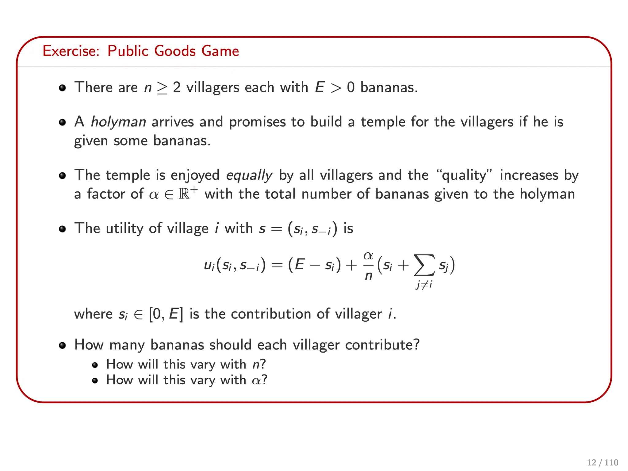
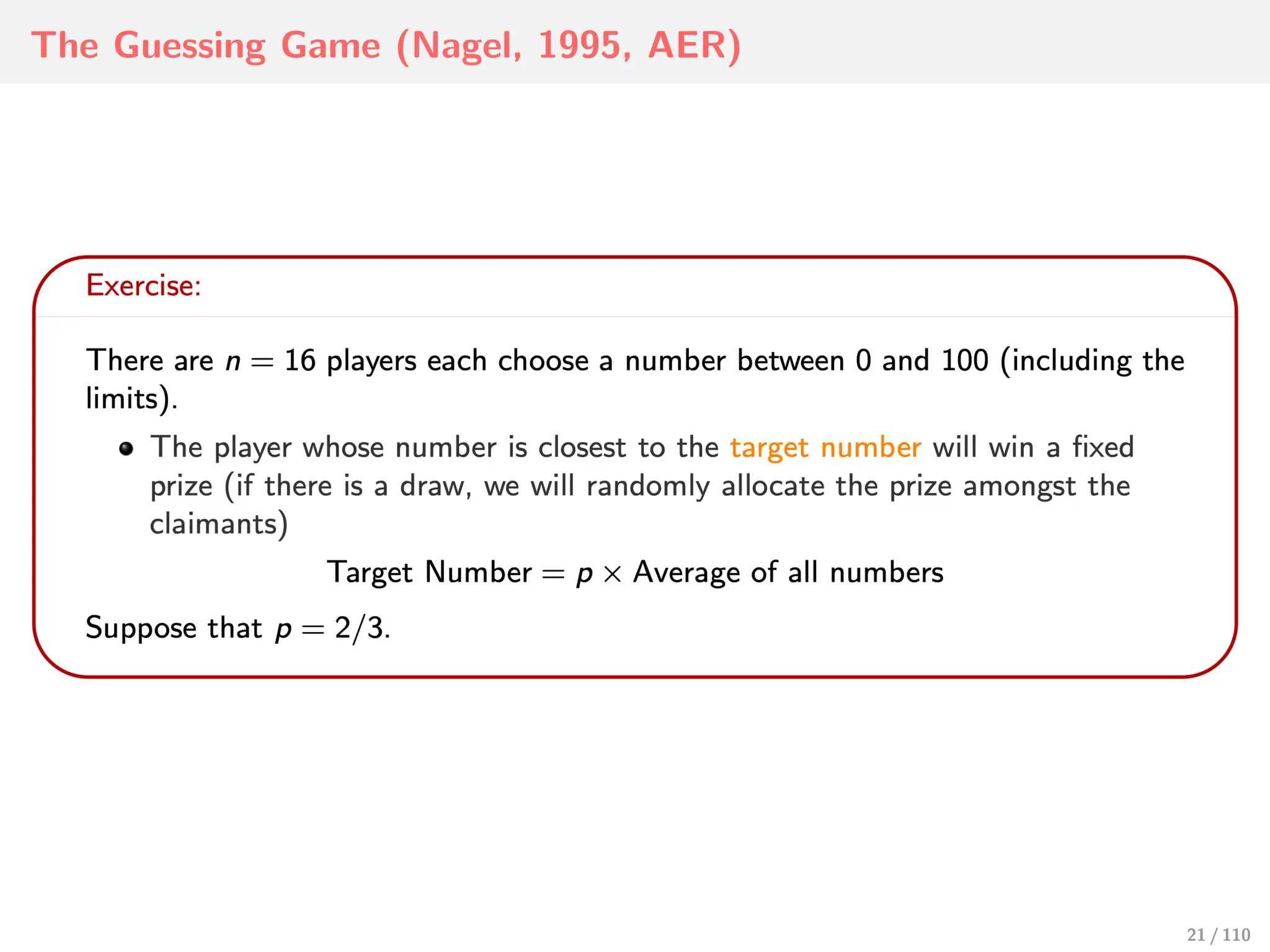
Exercise:
⊲ What does it mean to play one–shot?
⊲ What does complete information mean?
⊲ What does it mean to act simultaneously?
4 / 110
5.
What is agame?
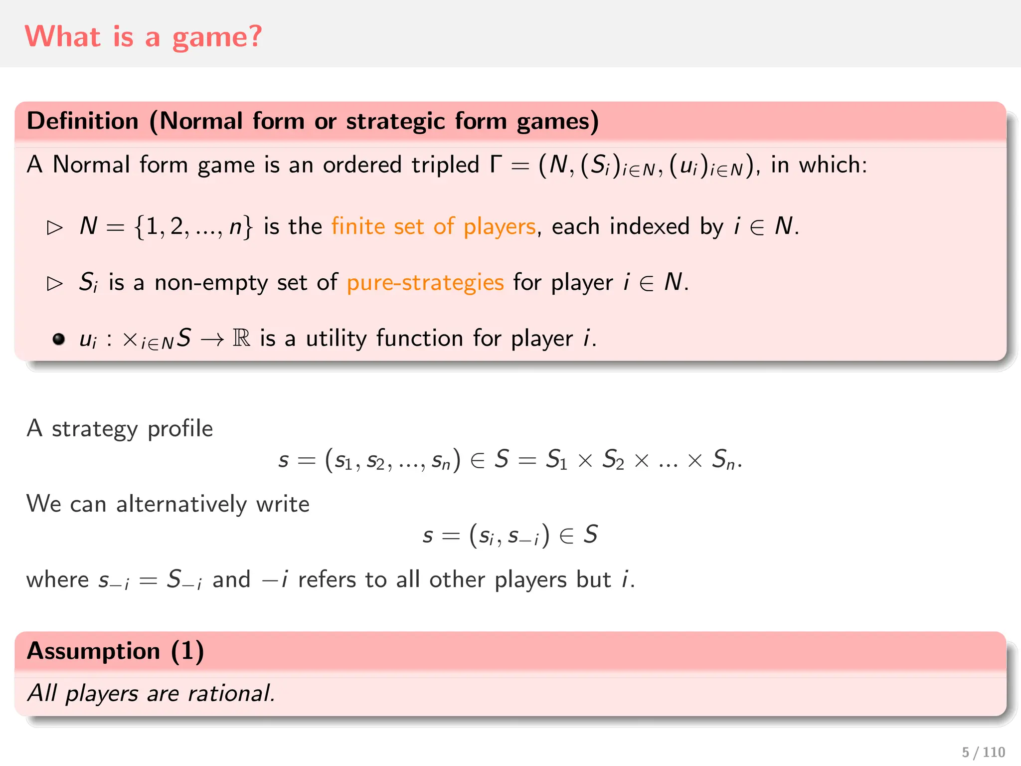
Definition (Normal form or strategic form games)
A Normal form game is an ordered tripled Γ = (N, (Si )i∈N , (ui )i∈N ), in which:
⊲ N = {1, 2, ..., n} is the finite set of players, each indexed by i ∈ N.
⊲ Si is a non-empty set of pure-strategies for player i ∈ N.
ui : ×i∈N S → R is a utility function for player i.
A strategy profile
s = (s1, s2, ..., sn) ∈ S = S1 × S2 × ... × Sn.
We can alternatively write
s = (si , s−i ) ∈ S
where s−i = S−i and −i refers to all other players but i.
Assumption (1)
All players are rational.
5 / 110
6.
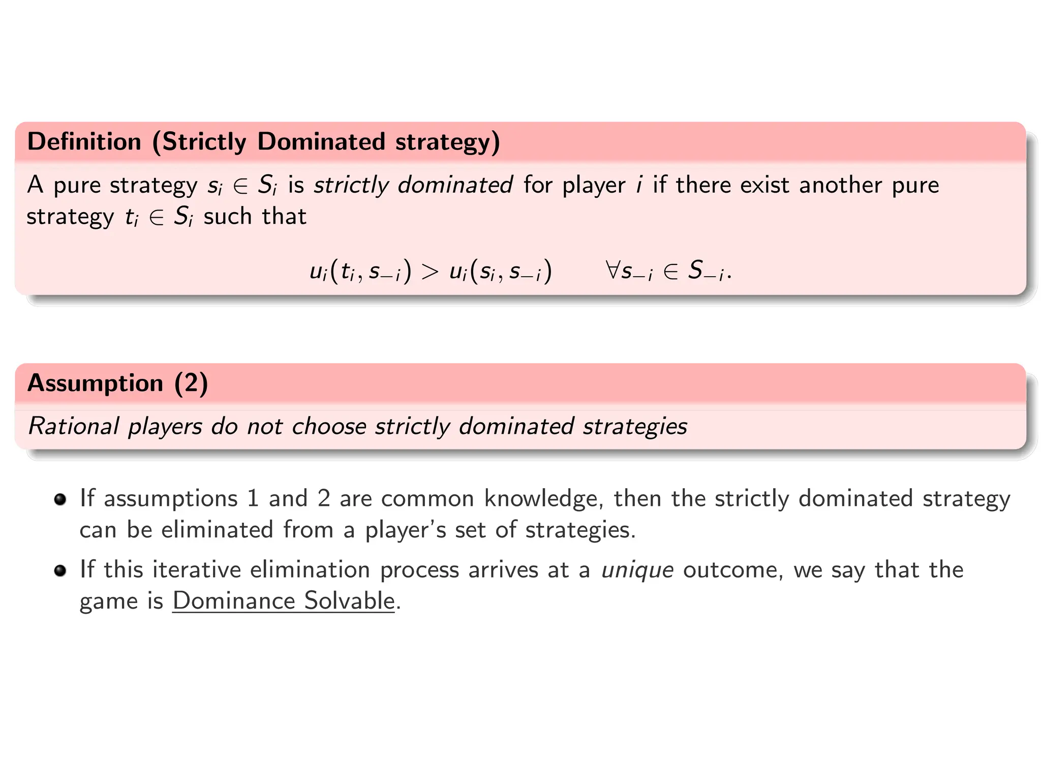
Definition (Strictly Dominatedstrategy)
A pure strategy si ∈ Si is strictly dominated for player i if there exist another pure
strategy ti ∈ Si such that
ui (ti , s−i ) > ui (si , s−i ) ∀s−i ∈ S−i .
Assumption (2)
Rational players do not choose strictly dominated strategies
If assumptions 1 and 2 are common knowledge, then the strictly dominated strategy
can be eliminated from a player’s set of strategies.
If this iterative elimination process arrives at a unique outcome, we say that the
game is Dominance Solvable.
7.
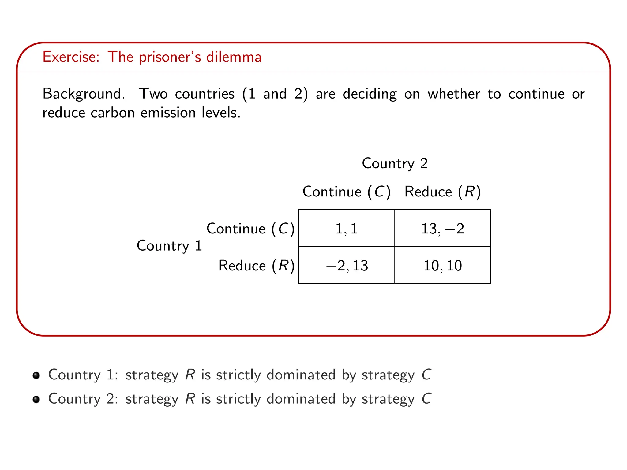
Exercise: The prisoner’sdilemma
Background. Two countries (1 and 2) are deciding on whether to continue or
reduce carbon emission levels.
Country 1
Country 2
Continue (C) Reduce (R)
Continue (C) 1, 1 13, −2
Reduce (R) −2, 13 10, 10
Country 1: strategy R is strictly dominated by strategy C
Country 2: strategy R is strictly dominated by strategy C
8.
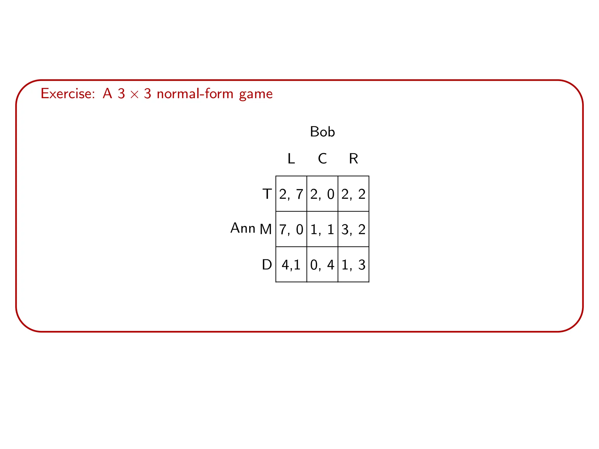
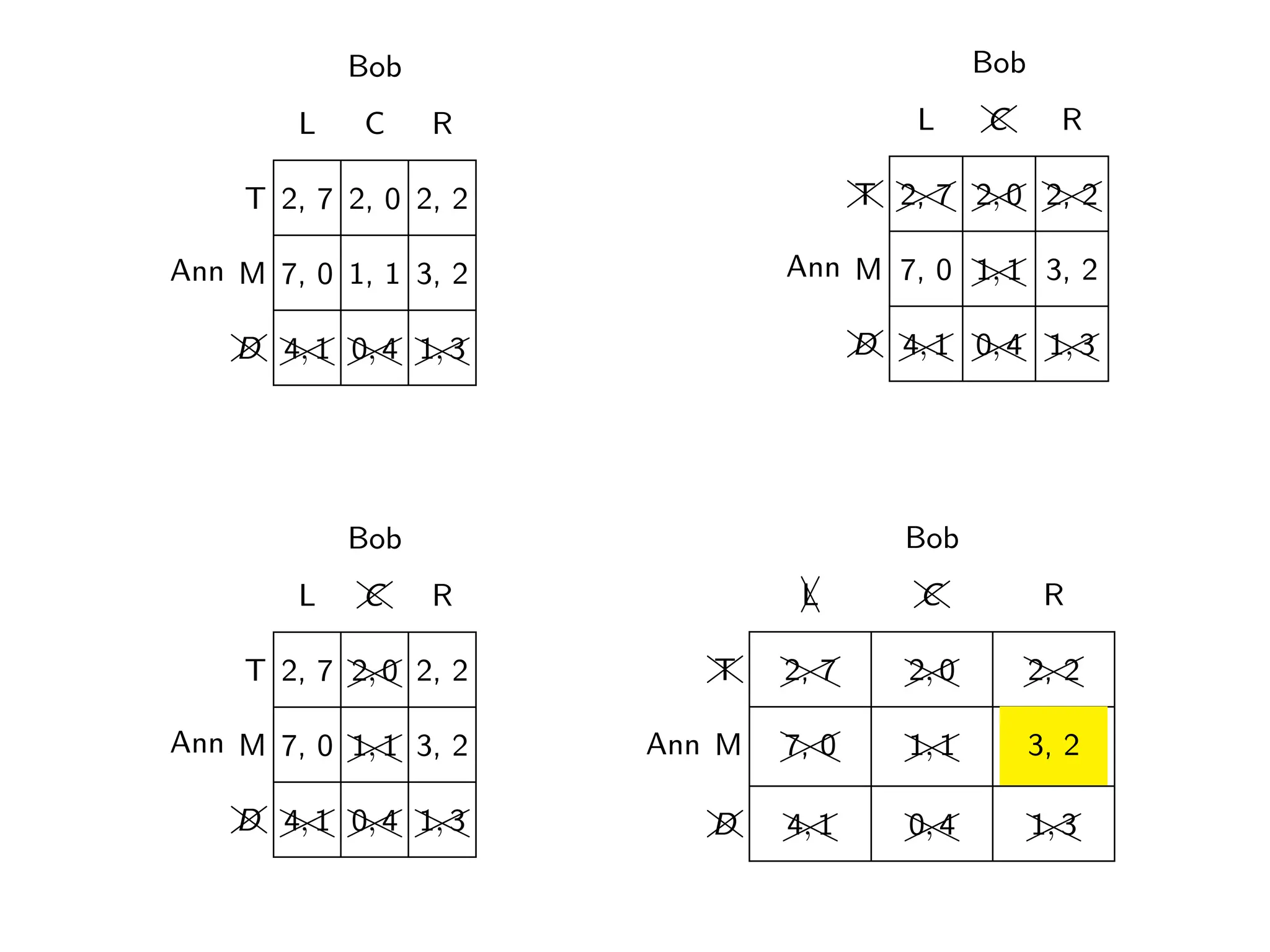
Exercise: A 3× 3 normal-form game
Ann
Bob
L C R
T 2, 7 2, 0 2, 2
M 7, 0 1, 1 3, 2
D 4,1 0, 4 1, 3
9.
Ann
Bob
L C R
T2, 7 2, 0 2, 2
M 7, 0 1, 1 3, 2
✚
❩
D ✟
✟
❍
❍
4, 1 ✟
✟
❍
❍
0, 4 ✟
✟
❍
❍
1, 3
Ann
Bob
L ✚
❩
C R
T 2, 7 ✟
✟
❍
❍
2, 0 2, 2
M 7, 0 ✟
✟
❍
❍
1, 1 3, 2
✚
❩
D ✟
✟
❍
❍
4, 1 ✟
✟
❍
❍
0, 4 ✟
✟
❍
❍
1, 3
Ann
Bob
L ✚
❩
C R
✚
❩
T ✟
✟
❍
❍
2, 7 ✟
✟
❍
❍
2, 0 ✟
✟
❍
❍
2, 2
M 7, 0 ✟
✟
❍
❍
1, 1 3, 2
✚
❩
D ✟
✟
❍
❍
4, 1 ✟
✟
❍
❍
0, 4 ✟
✟
❍
❍
1, 3
Ann
Bob
✁
❆
L ✚
❩
C R
✚
❩
T ✟
✟
❍
❍
2, 7 ✟
✟
❍
❍
2, 0 ✟
✟
❍
❍
2, 2
M ✟
✟
❍
❍
7, 0 ✟
✟
❍
❍
1, 1 3, 2
✚
❩
D ✟
✟
❍
❍
4, 1 ✟
✟
❍
❍
0, 4 ✟
✟
❍
❍
1, 3
10.
Nash Equilibrium (NE)
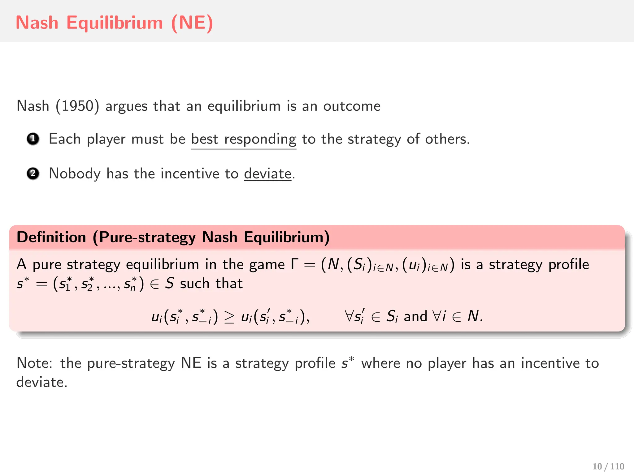
Nash(1950) argues that an equilibrium is an outcome
Each player must be best responding to the strategy of others.
Nobody has the incentive to deviate.
Definition (Pure-strategy Nash Equilibrium)
A pure strategy equilibrium in the game Γ = (N, (Si )i∈N , (ui )i∈N ) is a strategy profile
s∗
= (s∗
1 , s∗
2 , ..., s∗
n ) ∈ S such that
ui (s∗
i , s∗
−i ) ≥ ui (s′
i , s∗
−i ), ∀s′
i ∈ Si and ∀i ∈ N.
Note: the pure-strategy NE is a strategy profile s∗
where no player has an incentive to
deviate.
10 / 110
11.
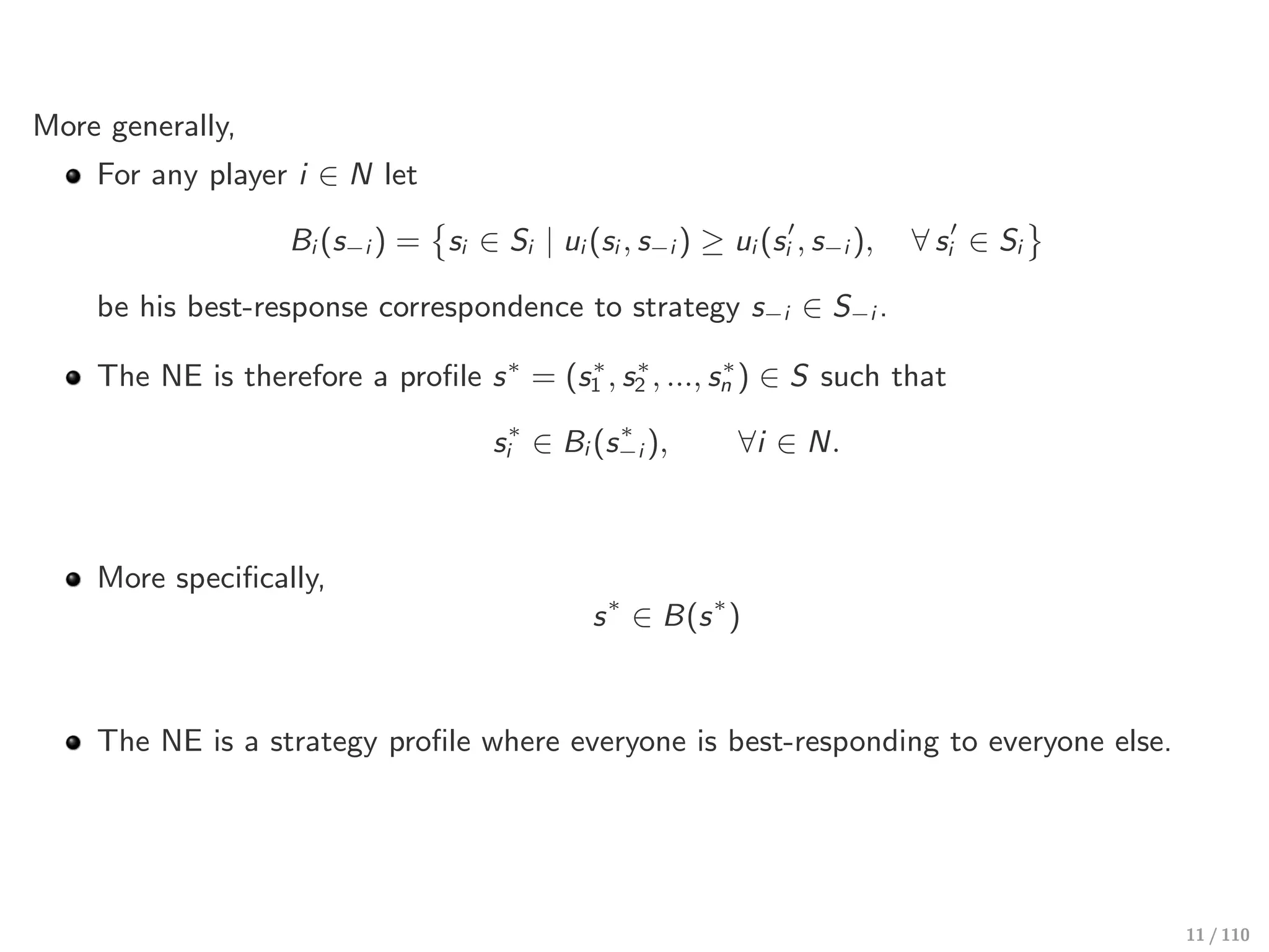
More generally,
For anyplayer i ∈ N let
Bi (s−i ) =
!
si ∈ Si | ui (si , s−i ) ≥ ui (s′
i , s−i ), ∀ s′
i ∈ Si
"
be his best-response correspondence to strategy s−i ∈ S−i .
The NE is therefore a profile s∗
= (s∗
1 , s∗
2 , ..., s∗
n ) ∈ S such that
s∗
i ∈ Bi (s∗
−i ), ∀i ∈ N.
More specifically,
s∗
∈ B(s∗
)
The NE is a strategy profile where everyone is best-responding to everyone else.
11 / 110
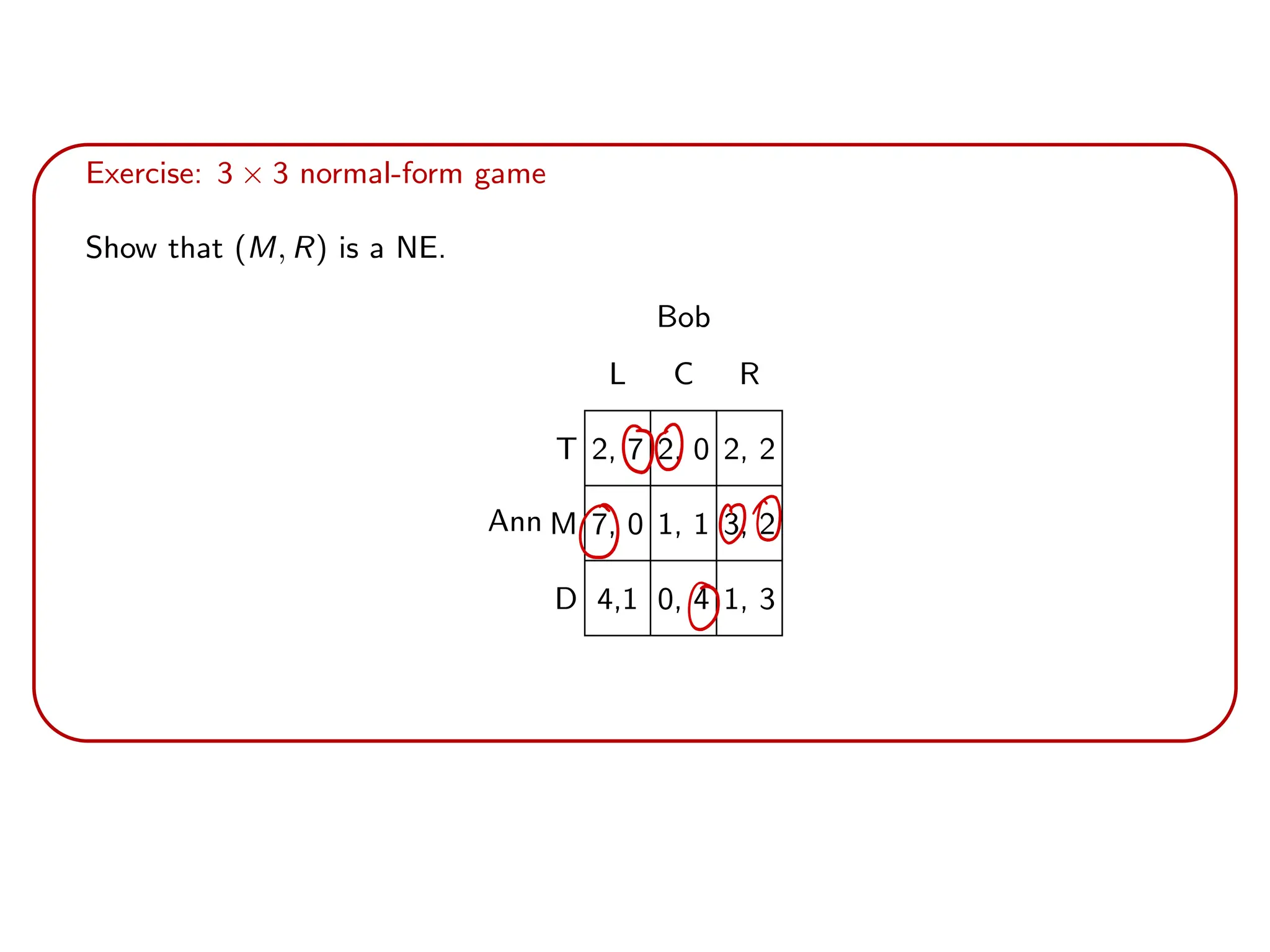
Exercise: 3 ×3 normal-form game
Show that (M, R) is a NE.
Ann
Bob
L C R
T 2, 7 2, 0 2, 2
M 7, 0 1, 1 3, 2
D 4,1 0, 4 1, 3
00
000
O
14.
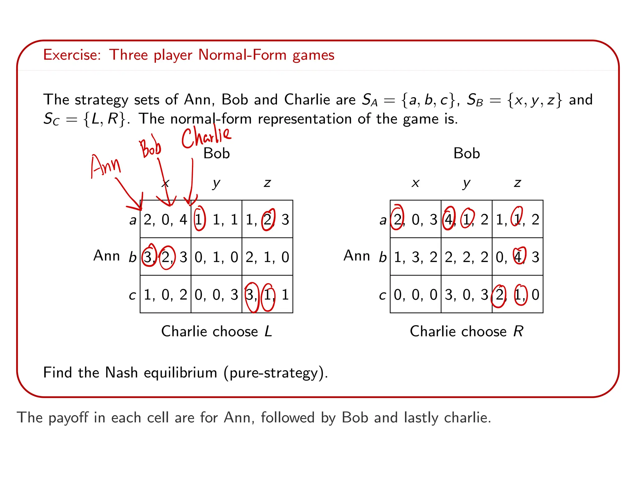
Exercise: Three playerNormal-Form games
The strategy sets of Ann, Bob and Charlie are SA = {a, b, c}, SB = {x, y, z} and
SC = {L, R}. The normal-form representation of the game is.
Ann
Bob
x y z
a 2, 0, 4 1, 1, 1 1, 2, 3
b 3, 2, 3 0, 1, 0 2, 1, 0
c 1, 0, 2 0, 0, 3 3, 1, 1
Charlie choose L
Ann
Bob
x y z
a 2, 0, 3 4, 1, 2 1, 1, 2
b 1, 3, 2 2, 2, 2 0, 4, 3
c 0, 0, 0 3, 0, 3 2, 1, 0
Charlie choose R
Find the Nash equilibrium (pure-strategy).
The payoff in each cell are for Ann, followed by Bob and lastly charlie.
AnyBobCharles
00 0 00 O
00 O
00 00
15.
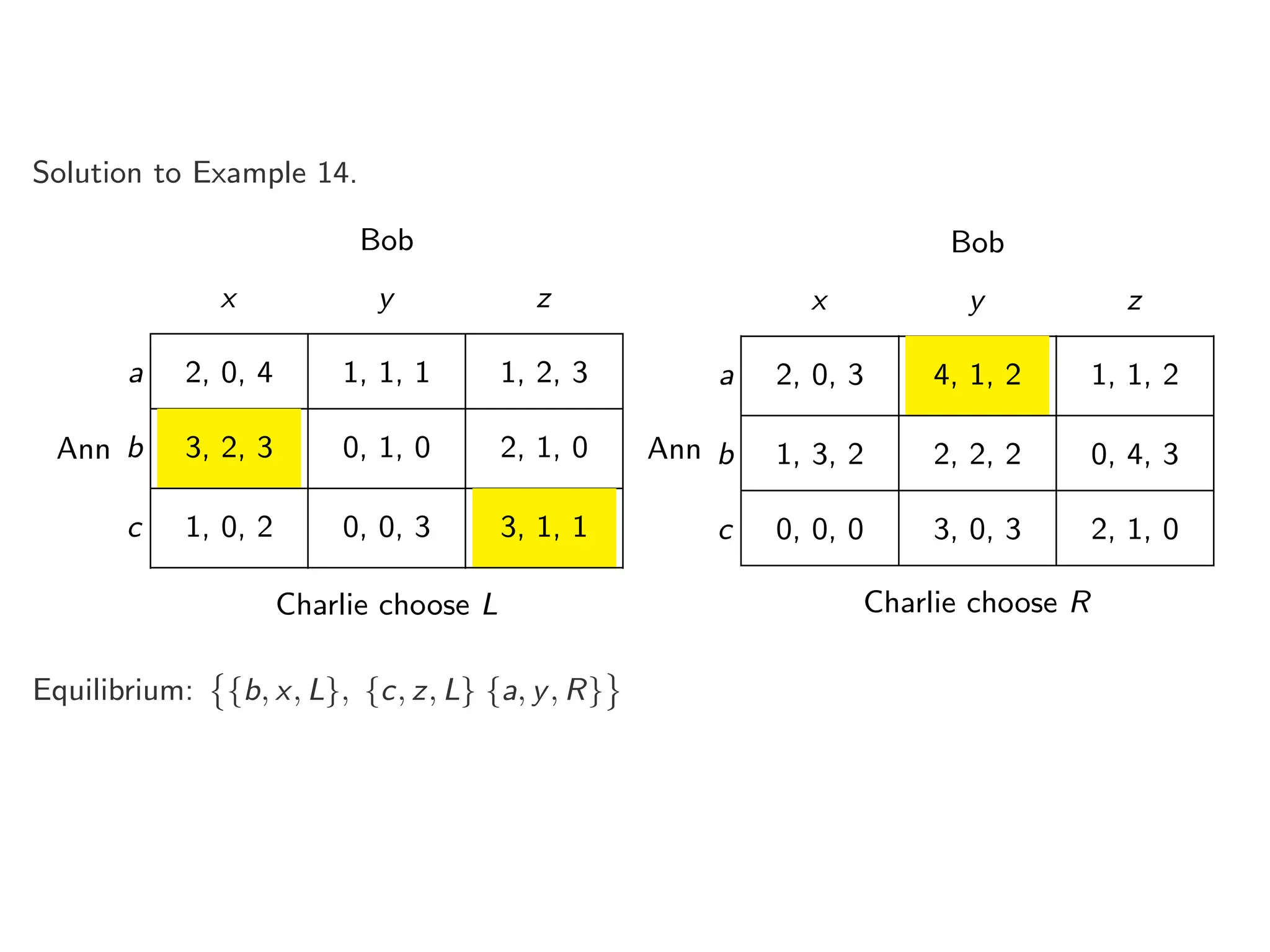
Solution to Example14.
Ann
Bob
x y z
a 2, 0, 4 1, 1, 1 1, 2, 3
b 3, 2, 3 0, 1, 0 2, 1, 0
c 1, 0, 2 0, 0, 3 3, 1, 1
Charlie choose L
Ann
Bob
x y z
a 2, 0, 3 4, 1, 2 1, 1, 2
b 1, 3, 2 2, 2, 2 0, 4, 3
c 0, 0, 0 3, 0, 3 2, 1, 0
Charlie choose R
Equilibrium:
!
{b, x, L}, {c, z, L} {a, y, R}
"
16.
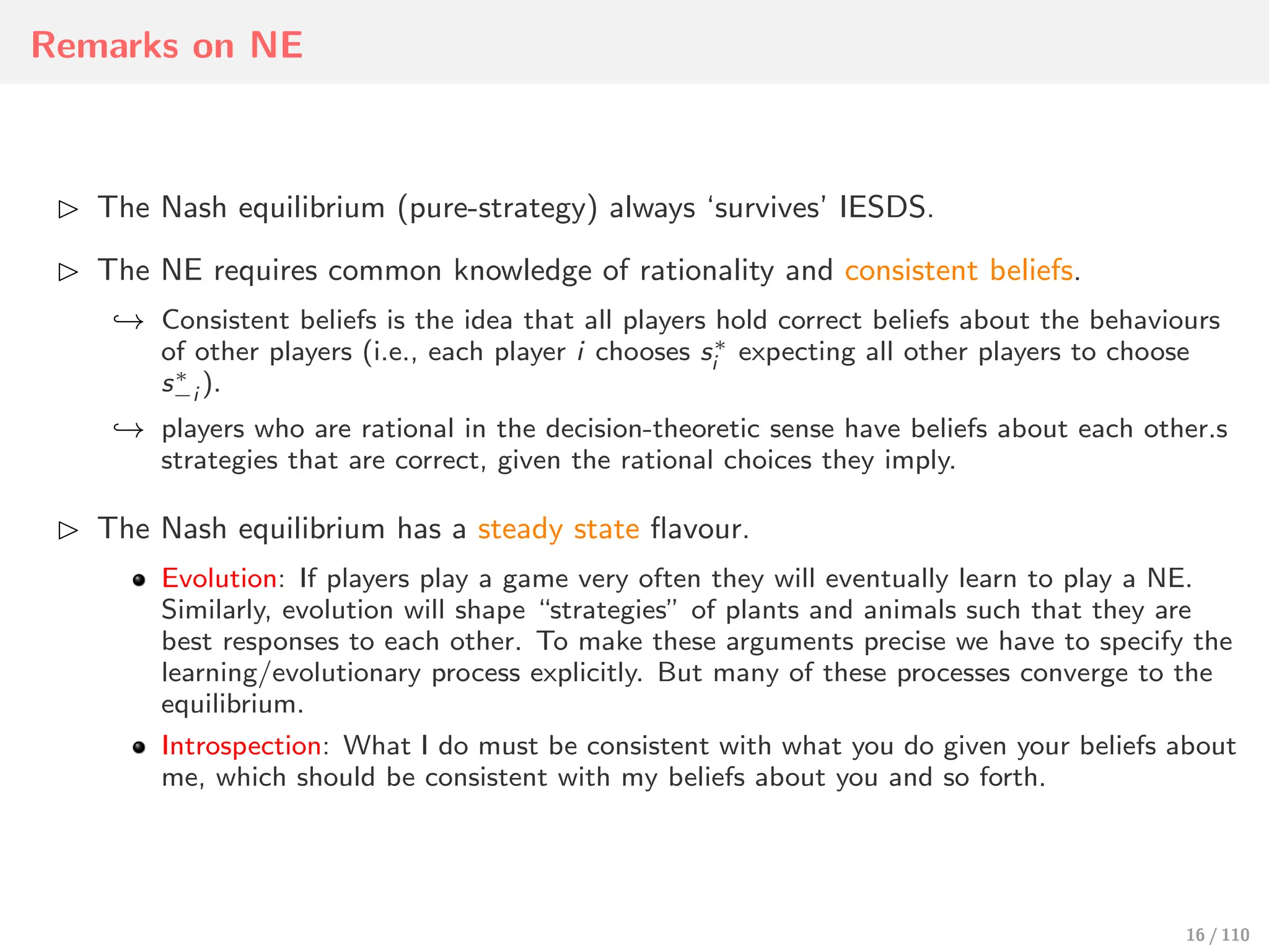
Remarks on NE
⊲The Nash equilibrium (pure-strategy) always ‘survives’ IESDS.
⊲ The NE requires common knowledge of rationality and consistent beliefs.
↩→ Consistent beliefs is the idea that all players hold correct beliefs about the behaviours
of other players (i.e., each player i chooses s∗
i expecting all other players to choose
s∗
−i ).
↩→ players who are rational in the decision-theoretic sense have beliefs about each other.s
strategies that are correct, given the rational choices they imply.
⊲ The Nash equilibrium has a steady state flavour.
Evolution: If players play a game very often they will eventually learn to play a NE.
Similarly, evolution will shape “strategies” of plants and animals such that they are
best responses to each other. To make these arguments precise we have to specify the
learning/evolutionary process explicitly. But many of these processes converge to the
equilibrium.
Introspection: What I do must be consistent with what you do given your beliefs about
me, which should be consistent with my beliefs about you and so forth.
16 / 110
17.
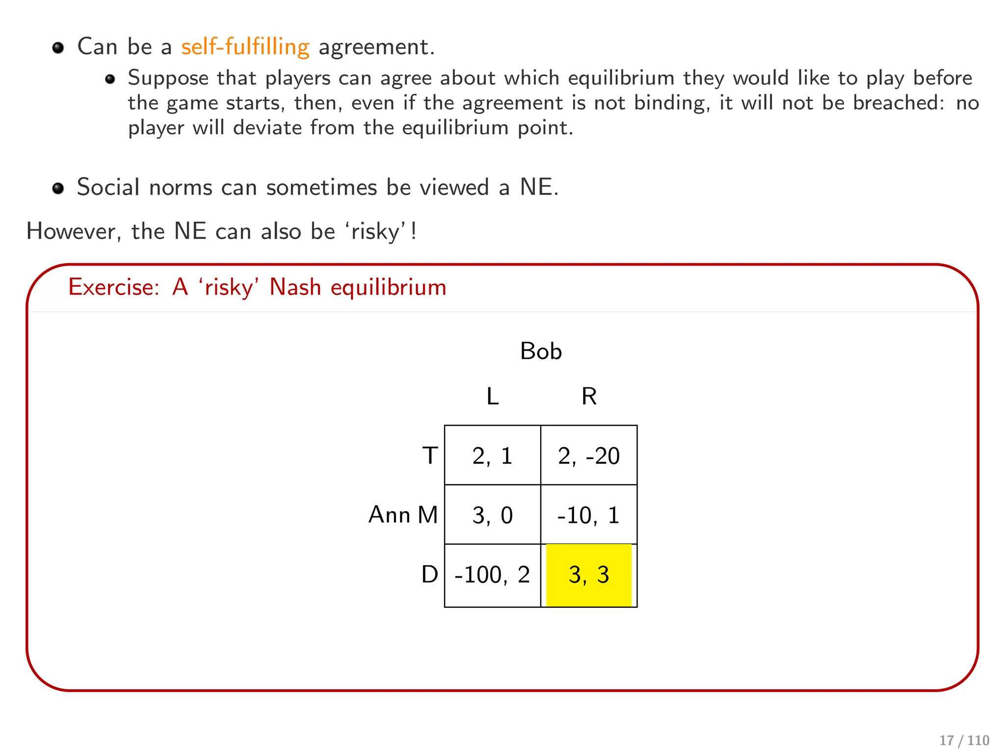
Can be aself-fulfilling agreement.
Suppose that players can agree about which equilibrium they would like to play before
the game starts, then, even if the agreement is not binding, it will not be breached: no
player will deviate from the equilibrium point.
Social norms can sometimes be viewed a NE.
However, the NE can also be ‘risky’!
Exercise: A ‘risky’ Nash equilibrium
Ann
Bob
L R
T 2, 1 2, -20
M 3, 0 -10, 1
D -100, 2 3, 3
17 / 110
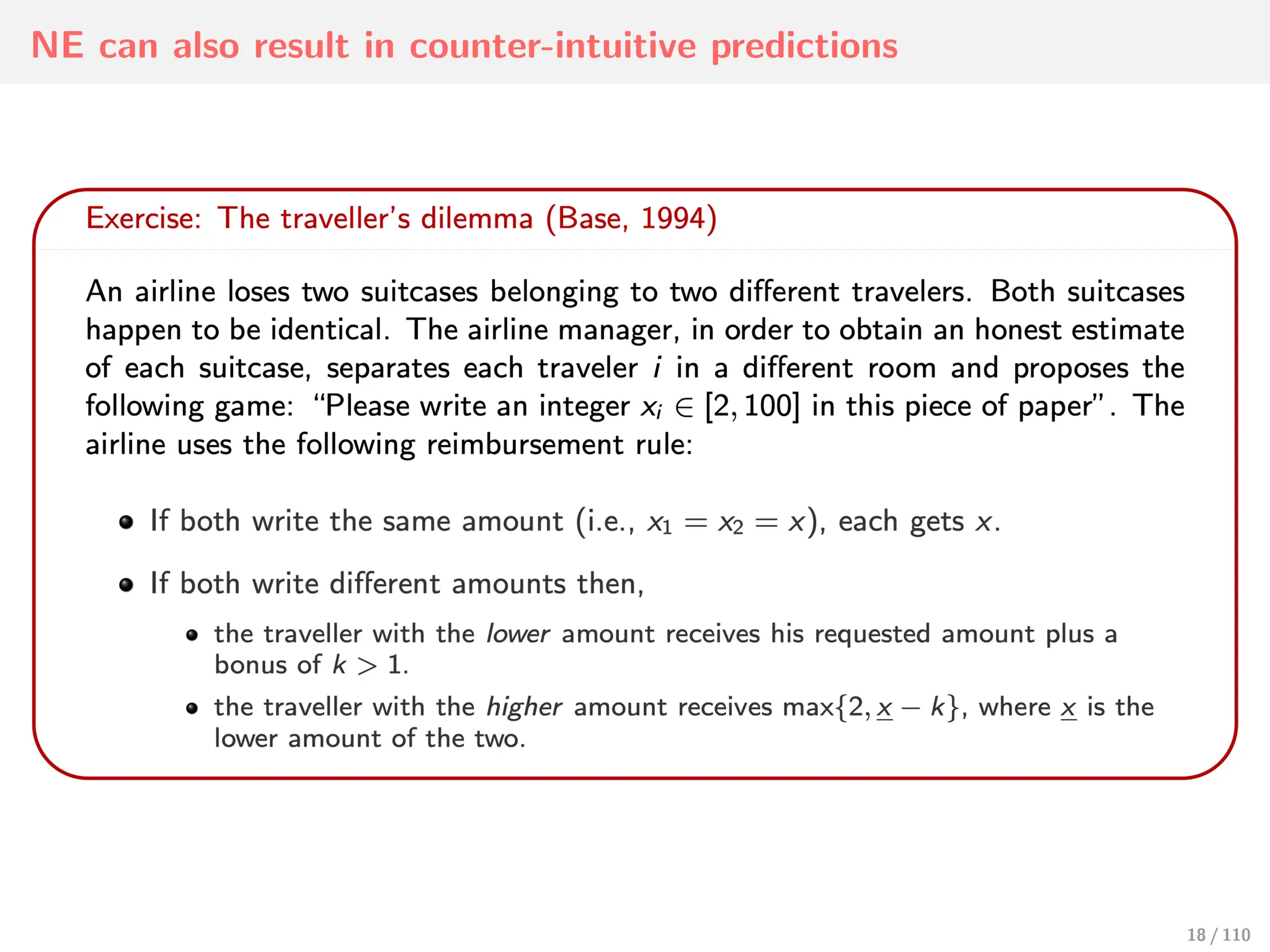
18.
NE can alsoresult in counter-intuitive predictions
18 / 110
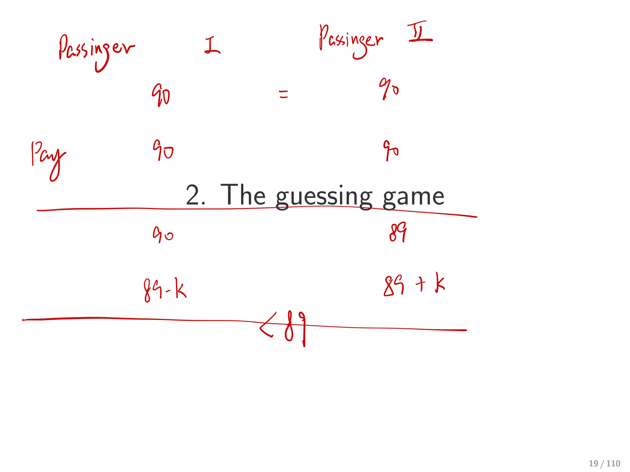
19.
2. The guessinggame
19 / 110
Passinger 2 Passinger E
90 I 90
go
I
20.
Keynes Beauty contest
⊲Consider a fictional newspaper contest, in which entrants are asked to choose the six
most attractive faces from a hundred photographs. Those who picked the most
popular faces are then eligible for a prize.
“It is not a case of choosing those [faces] that, to the best of one’s judgment,
are really the prettiest, nor even those that average opinion genuinely thinks the
prettiest.
We have reached the third degree where we devote our intelligences to anticipat-
ing what average opinion expects the average opinion to be.
And there are some, I believe, who practice the fourth, fifth and higher
degrees.”—(Keynes, General Theory of Employment, Interest and Money, 1936).
Exercise:
Can you think of economic situations that closely mirrors the beauty contest de-
scribed above?
20 / 110
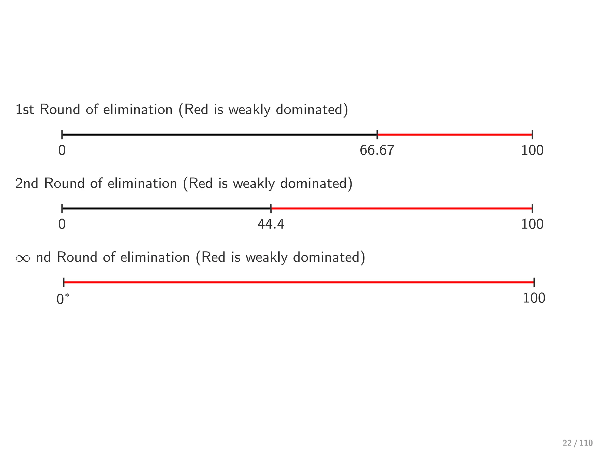
1st Round ofelimination (Red is weakly dominated)
0 100
66.67
2nd Round of elimination (Red is weakly dominated)
0 100
44.4
∞ nd Round of elimination (Red is weakly dominated)
100
0∗
22 / 110
23.
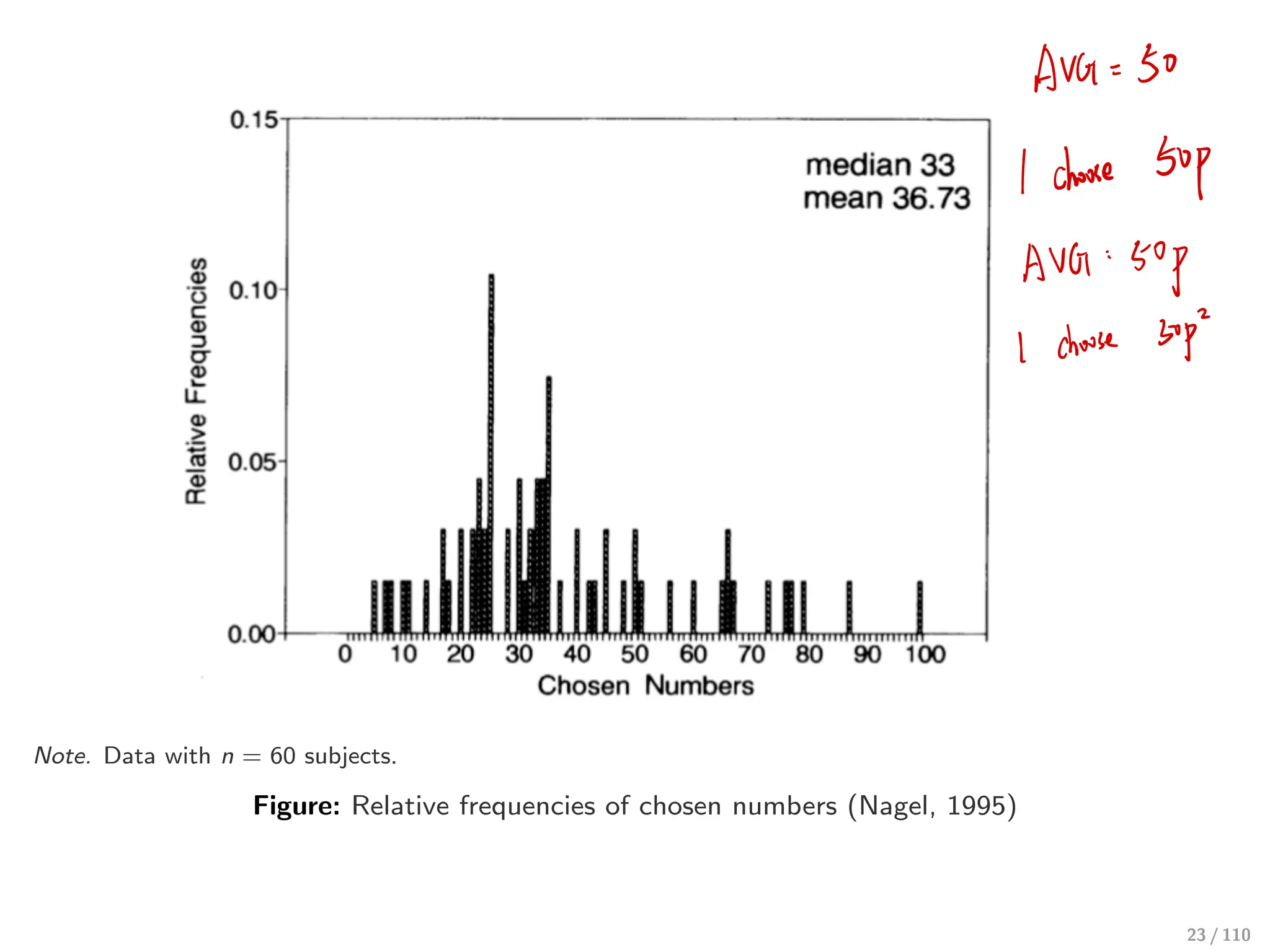
Note. Data withn = 60 subjects.
Figure: Relative frequencies of chosen numbers (Nagel, 1995)
23 / 110
AVG = 50
I choose 50p
AVG
:
Sop
I choose sop
24.
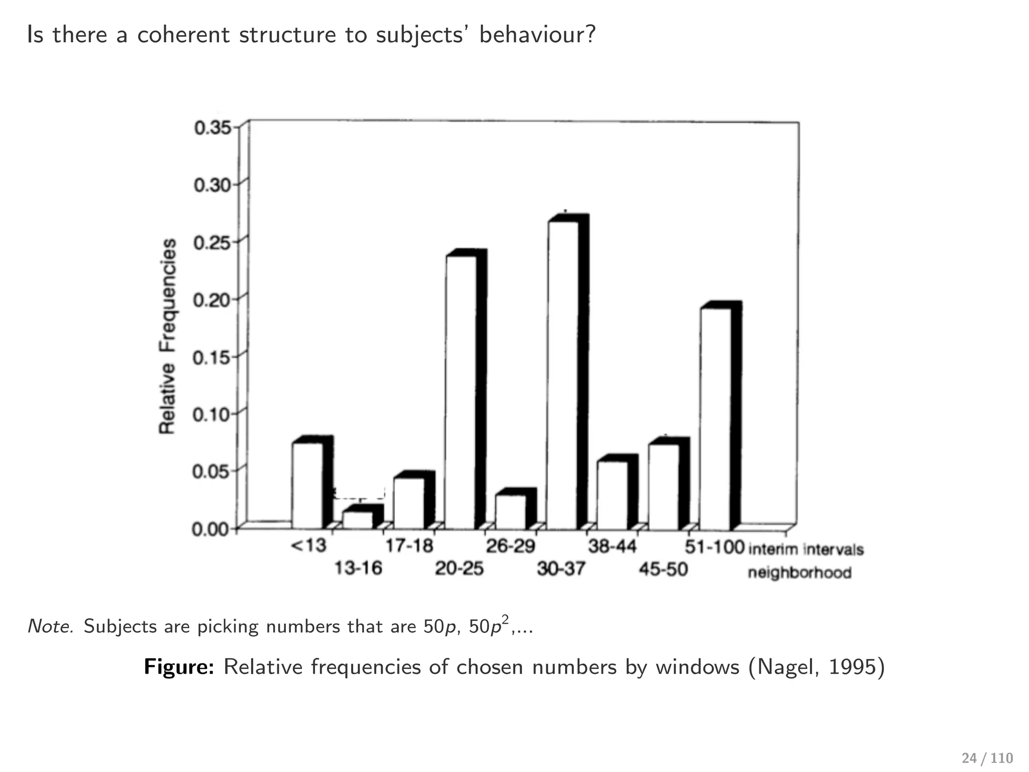
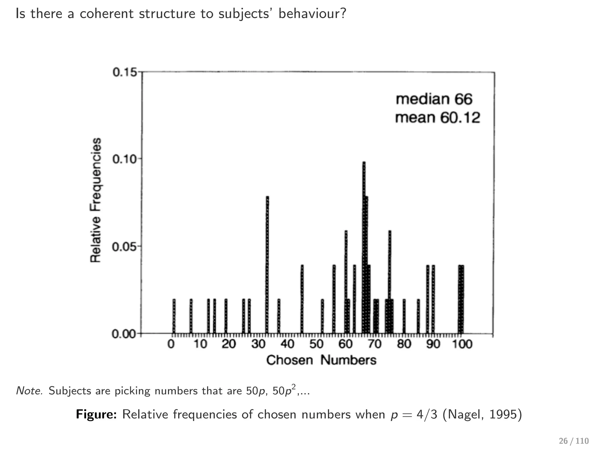
Is there acoherent structure to subjects’ behaviour?
Note. Subjects are picking numbers that are 50p, 50p2
,...
Figure: Relative frequencies of chosen numbers by windows (Nagel, 1995)
24 / 110
Is there acoherent structure to subjects’ behaviour?
Note. Subjects are picking numbers that are 50p, 50p2
,...
Figure: Relative frequencies of chosen numbers when p = 4/3 (Nagel, 1995)
26 / 110
27.
Bosch-Domenech, Montalvo, Nageland Satorra (2002, AER)
⊲ Nagel (1995) results raises pertinent questions about whether the observed
deviations from NE are unique to students.
⊲ Will the deviations still follow a systematic manner if we had:
↩→ larger numbers of subjects
↩→ larger rewards
↩→ longer decision time
↩→ more diverse subject pool than would be possible in the lab
27 / 110
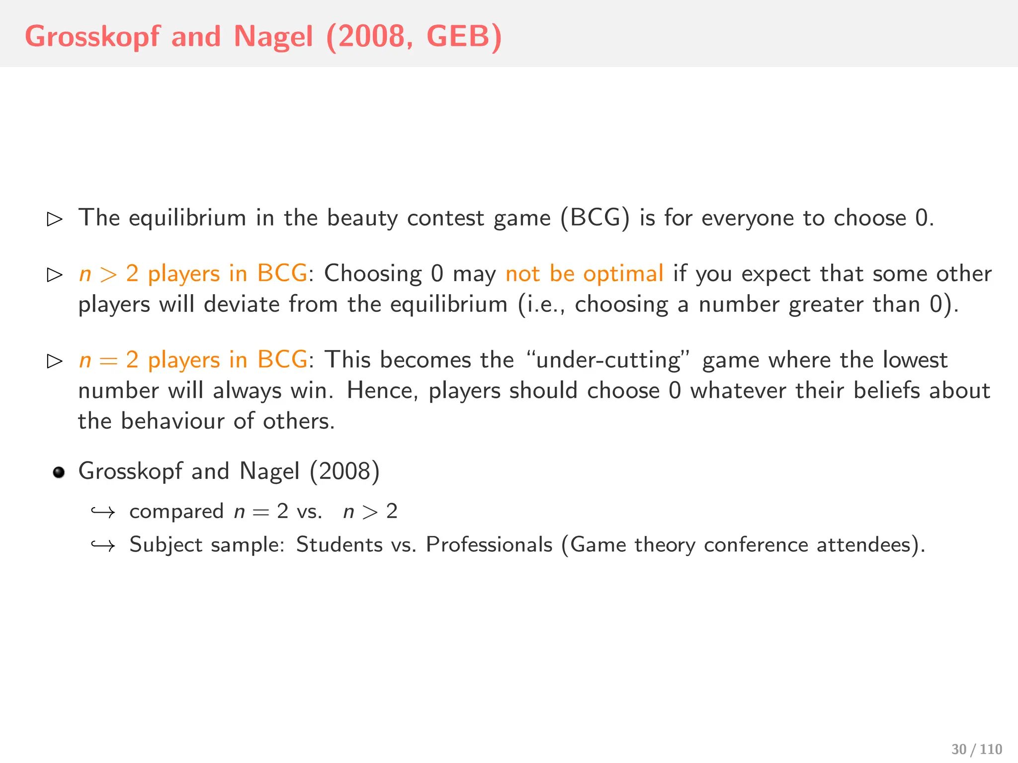
Grosskopf and Nagel(2008, GEB)
⊲ The equilibrium in the beauty contest game (BCG) is for everyone to choose 0.
⊲ n > 2 players in BCG: Choosing 0 may not be optimal if you expect that some other
players will deviate from the equilibrium (i.e., choosing a number greater than 0).
⊲ n = 2 players in BCG: This becomes the “under-cutting” game where the lowest
number will always win. Hence, players should choose 0 whatever their beliefs about
the behaviour of others.
Grosskopf and Nagel (2008)
↩→ compared n = 2 vs. n > 2
↩→ Subject sample: Students vs. Professionals (Game theory conference attendees).
30 / 110
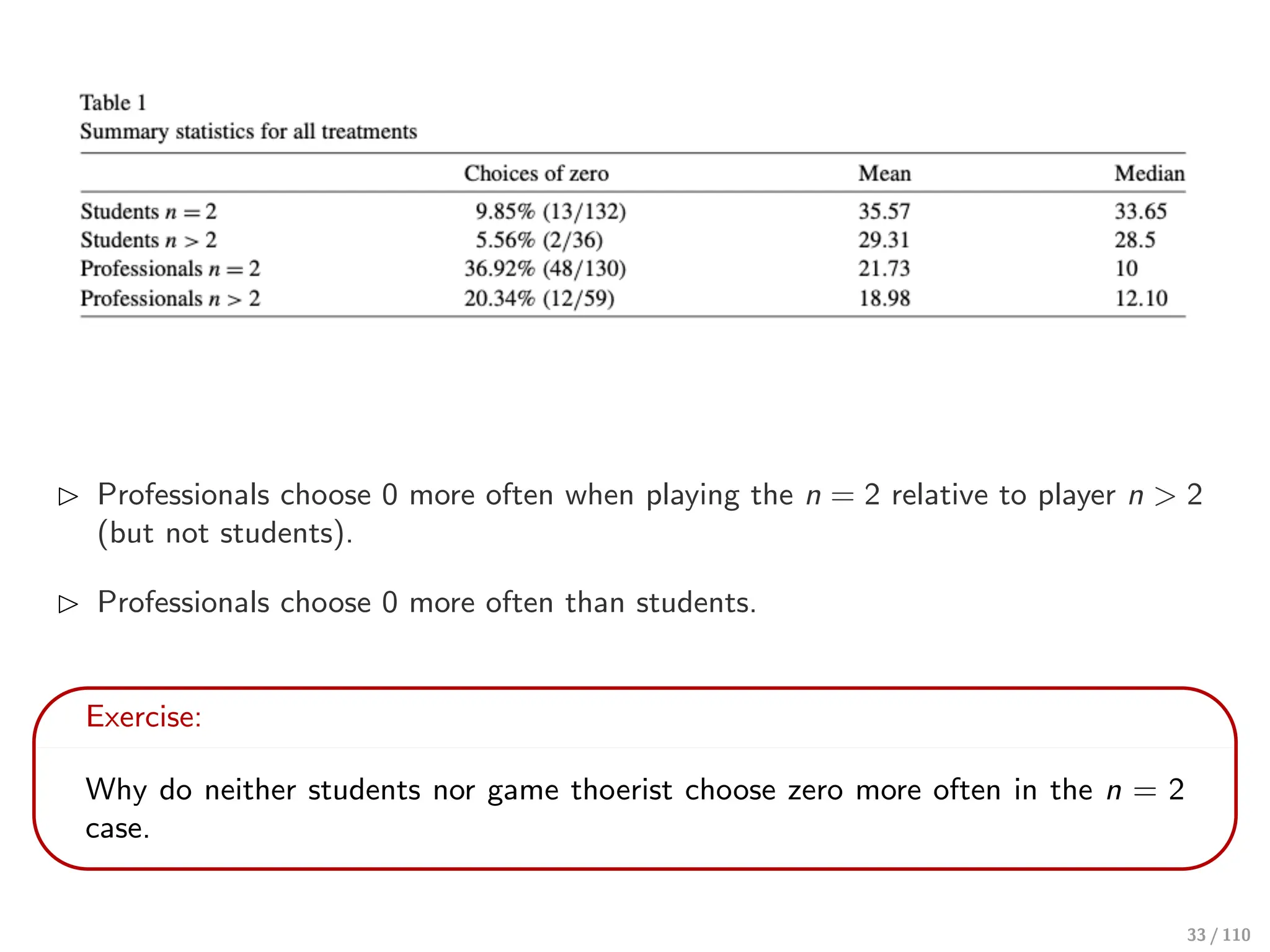
⊲ Professionals choose0 more often when playing the n = 2 relative to player n > 2
(but not students).
⊲ Professionals choose 0 more often than students.
Exercise:
Why do neither students nor game thoerist choose zero more often in the n = 2
case.
33 / 110
34.
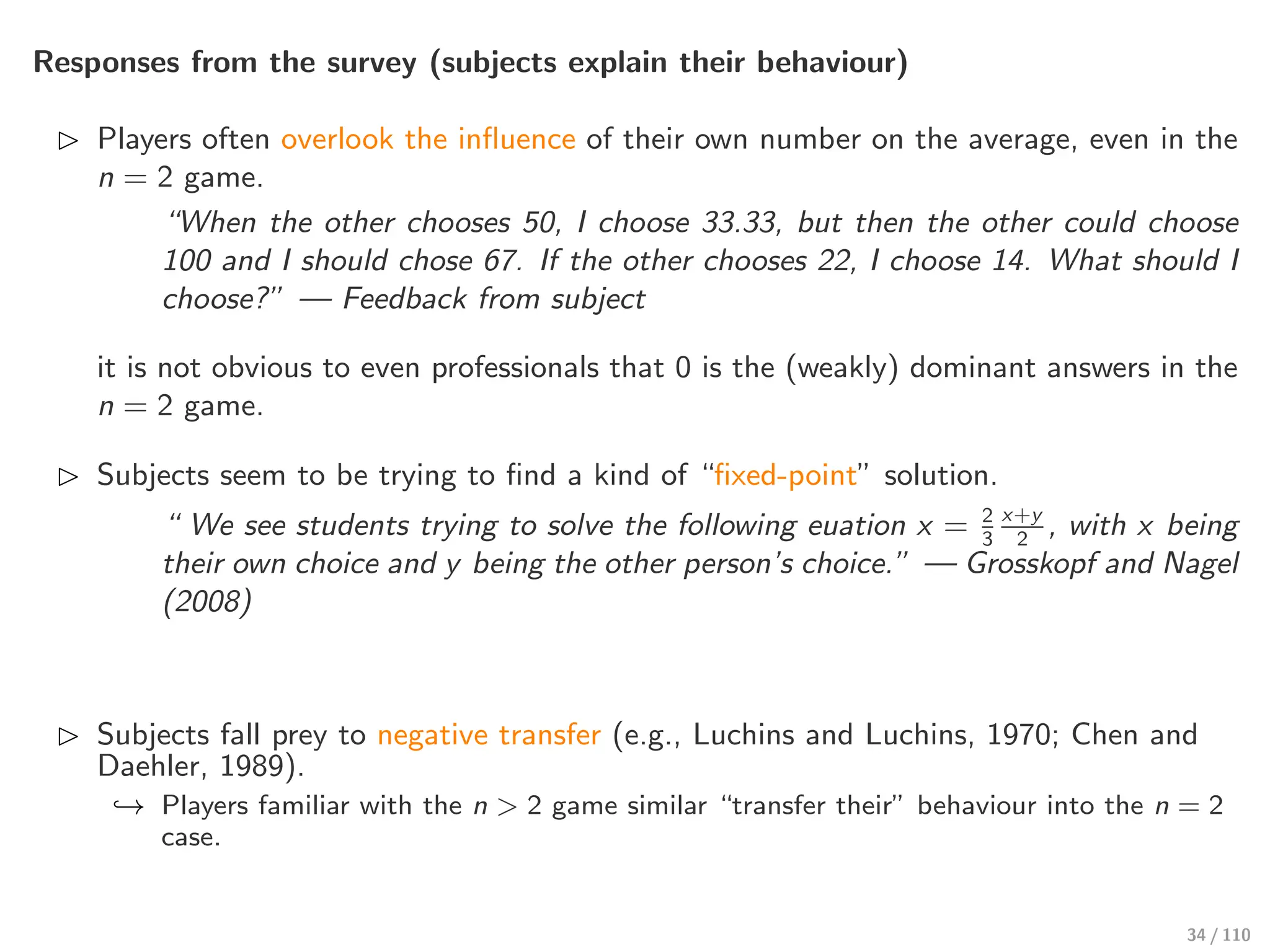
Responses from thesurvey (subjects explain their behaviour)
⊲ Players often overlook the influence of their own number on the average, even in the
n = 2 game.
“When the other chooses 50, I choose 33.33, but then the other could choose
100 and I should chose 67. If the other chooses 22, I choose 14. What should I
choose?” — Feedback from subject
it is not obvious to even professionals that 0 is the (weakly) dominant answers in the
n = 2 game.
⊲ Subjects seem to be trying to find a kind of “fixed-point” solution.
“ We see students trying to solve the following euation x = 2
3
x+y
2
, with x being
their own choice and y being the other person’s choice.” — Grosskopf and Nagel
(2008)
⊲ Subjects fall prey to negative transfer (e.g., Luchins and Luchins, 1970; Chen and
Daehler, 1989).
↩→ Players familiar with the n > 2 game similar “transfer their” behaviour into the n = 2
case.
34 / 110
Strategic thinking
The canonicalmodel of strategic thinking is the game-theoretic notion of Nash
equilibrium. Equilibrium is defined as a combination of strategies, one for each
player, such that each player’s strategy maximises his expected payoff, given the
others’ strategies.[...]
equilibrium is better justified in some applications than others. If players have
enough experience with analogous games, both theory and experimental results
suggest that learning has a strong tendency to converge to equilibrium.
If equilibrium is justified in such applications, it must be via strategic thinking
rather than learning.” — Crawford, Costa-Gomes and Iriberri (2013)
36 / 110
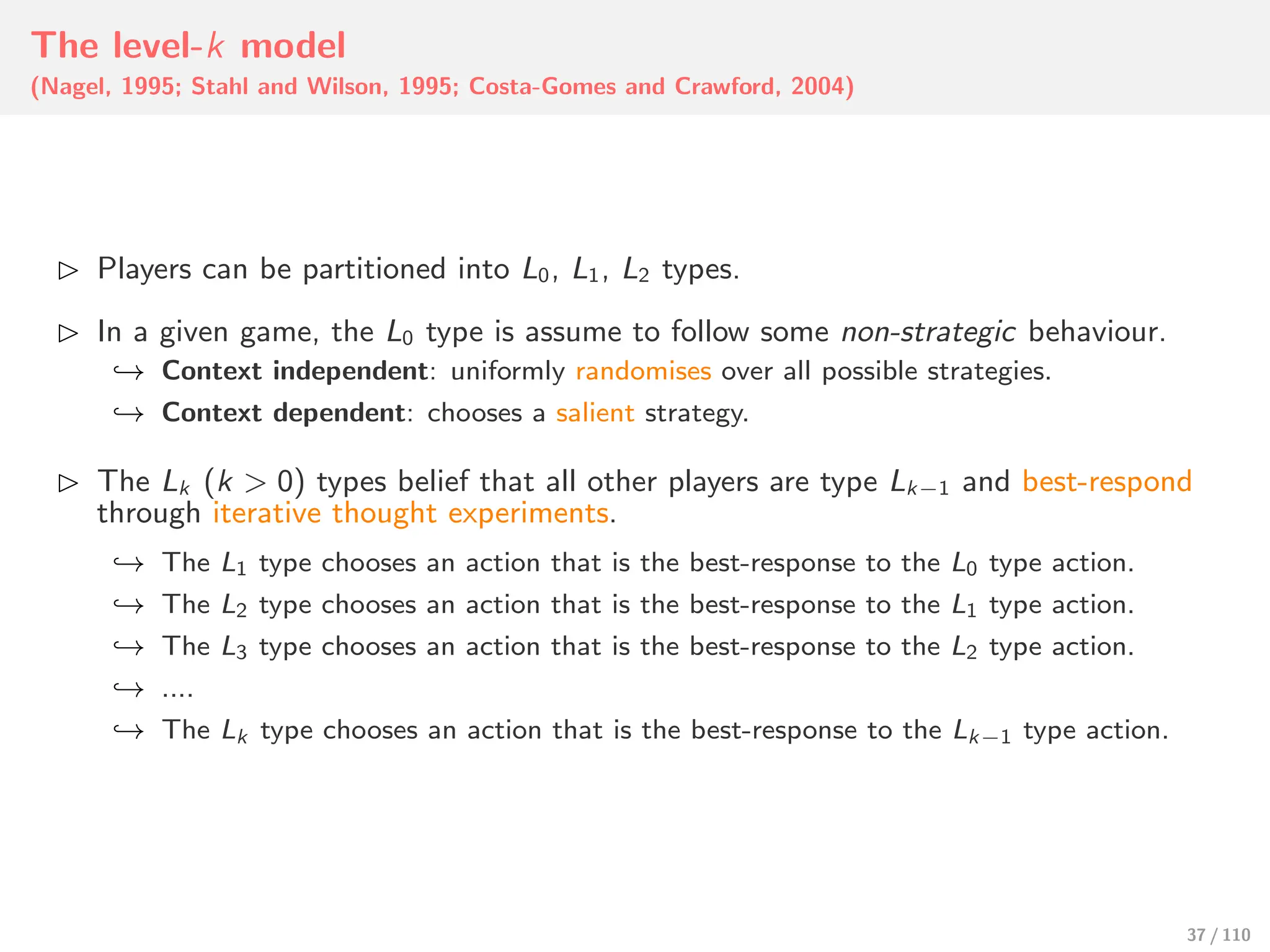
37.
The level-k model
(Nagel,1995; Stahl and Wilson, 1995; Costa-Gomes and Crawford, 2004)
⊲ Players can be partitioned into L0, L1, L2 types.
⊲ In a given game, the L0 type is assume to follow some non-strategic behaviour.
↩→ Context independent: uniformly randomises over all possible strategies.
↩→ Context dependent: chooses a salient strategy.
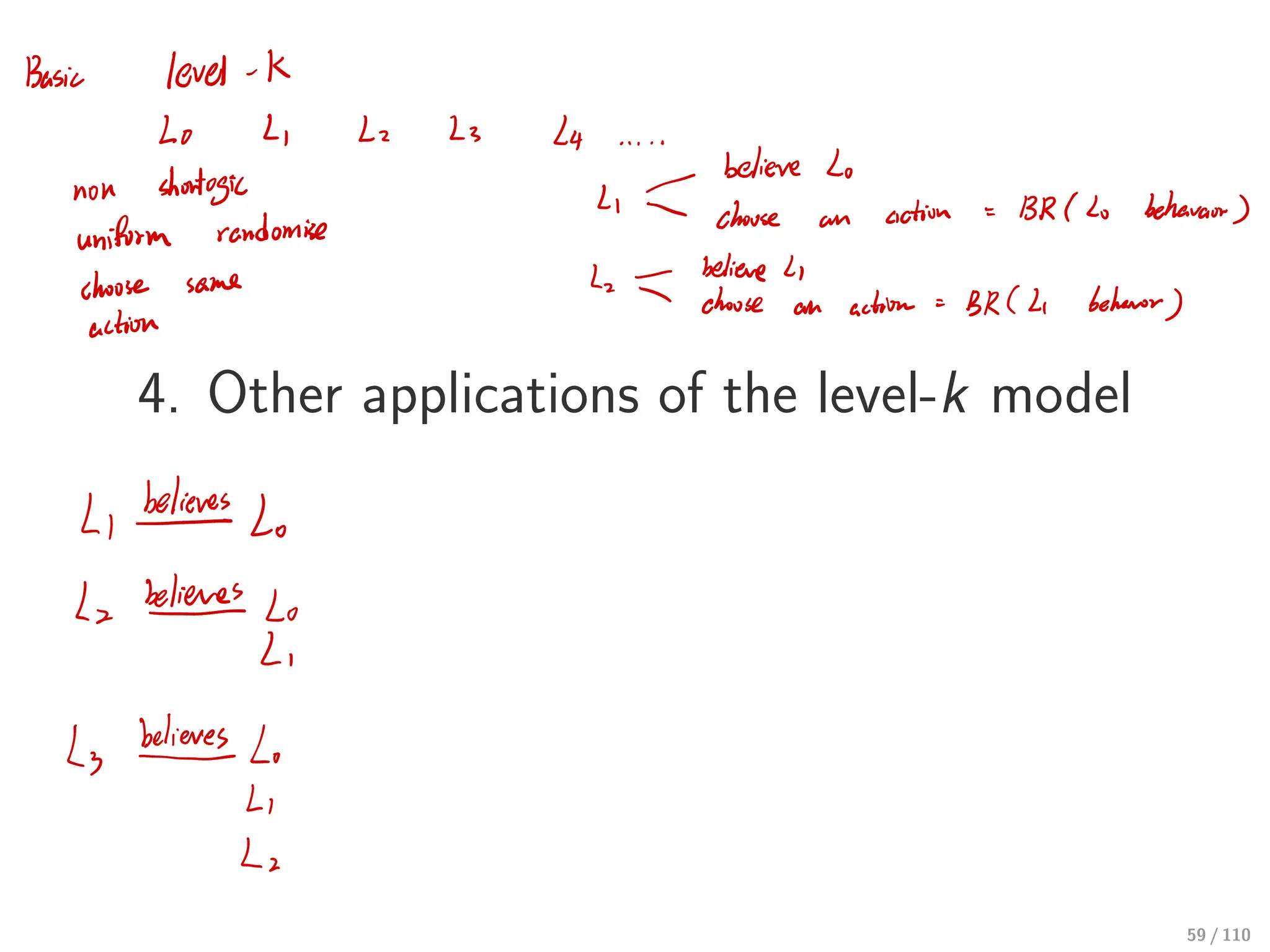
⊲ The Lk (k > 0) types belief that all other players are type Lk−1 and best-respond
through iterative thought experiments.
↩→ The L1 type chooses an action that is the best-response to the L0 type action.
↩→ The L2 type chooses an action that is the best-response to the L1 type action.
↩→ The L3 type chooses an action that is the best-response to the L2 type action.
↩→ ....
↩→ The Lk type chooses an action that is the best-response to the Lk−1 type action.
37 / 110
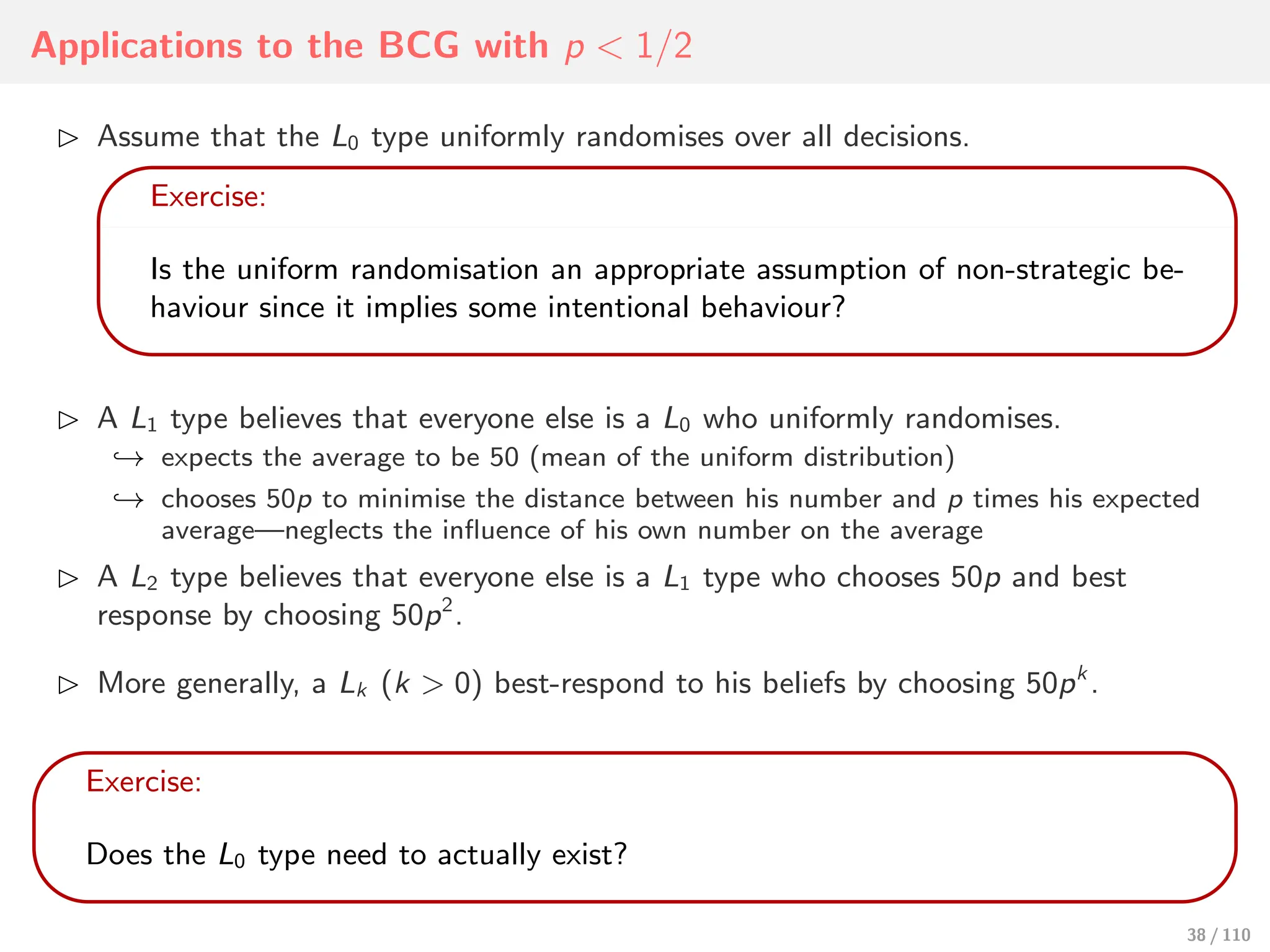
38.
Applications to theBCG with p < 1/2
⊲ Assume that the L0 type uniformly randomises over all decisions.
Exercise:
Is the uniform randomisation an appropriate assumption of non-strategic be-
haviour since it implies some intentional behaviour?
⊲ A L1 type believes that everyone else is a L0 who uniformly randomises.
↩→ expects the average to be 50 (mean of the uniform distribution)
↩→ chooses 50p to minimise the distance between his number and p times his expected
average—neglects the influence of his own number on the average
⊲ A L2 type believes that everyone else is a L1 type who chooses 50p and best
response by choosing 50p2
.
⊲ More generally, a Lk (k > 0) best-respond to his beliefs by choosing 50pk
.
Exercise:
Does the L0 type need to actually exist?
38 / 110
39.
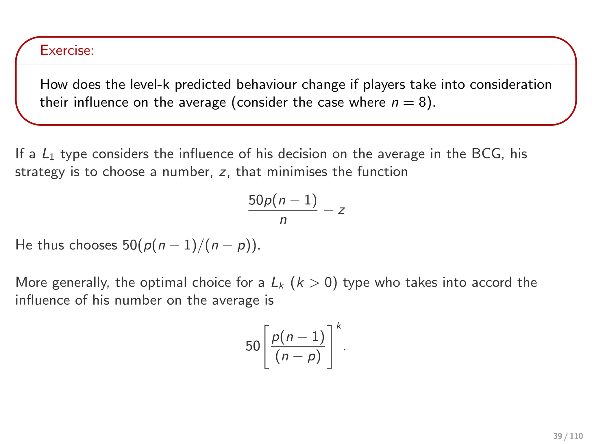
Exercise:
How does thelevel-k predicted behaviour change if players take into consideration
their influence on the average (consider the case where n = 8).
If a L1 type considers the influence of his decision on the average in the BCG, his
strategy is to choose a number, z, that minimises the function
50p(n − 1)
n
− z
He thus chooses 50(p(n − 1)/(n − p)).
More generally, the optimal choice for a Lk (k > 0) type who takes into accord the
influence of his number on the average is
50
#
p(n − 1)
(n − p)
$k
.
39 / 110
40.
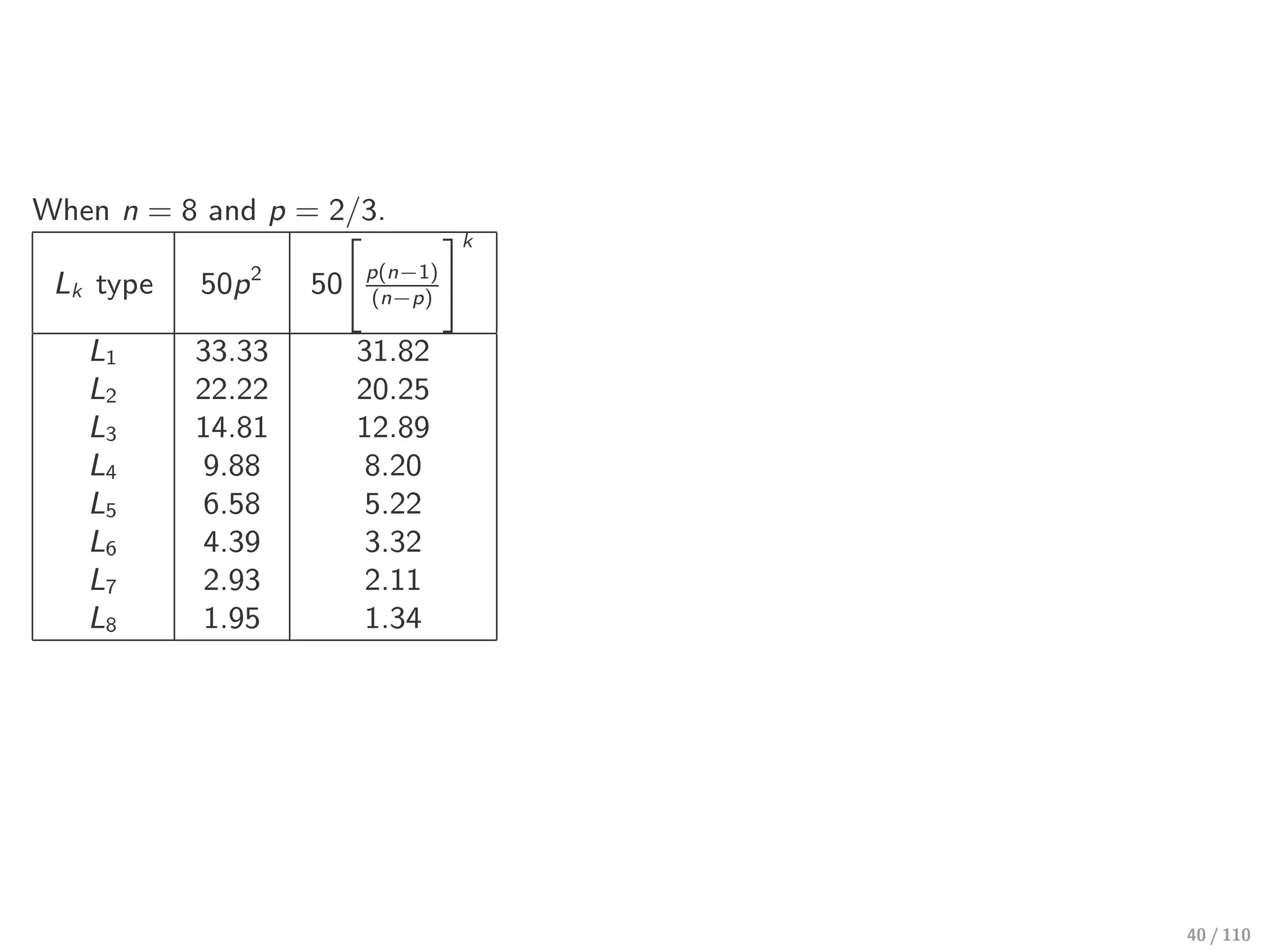
When n =8 and p = 2/3.
Lk type 50p2
50
#
p(n−1)
(n−p)
$k
L1 33.33 31.82
L2 22.22 20.25
L3 14.81 12.89
L4 9.88 8.20
L5 6.58 5.22
L6 4.39 3.32
L7 2.93 2.11
L8 1.95 1.34
40 / 110
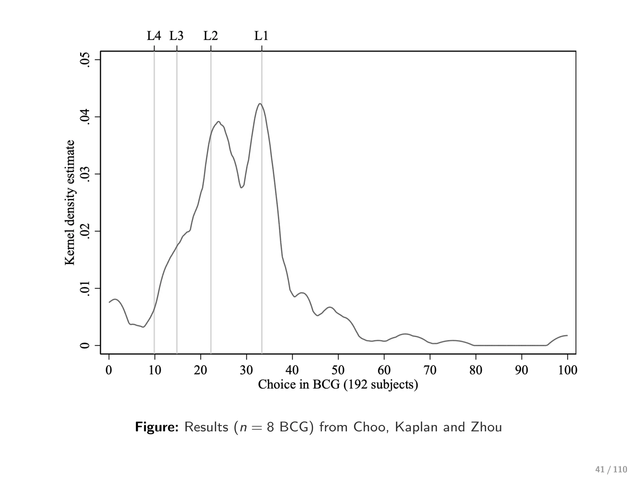
Individual vs. Aggregatelevel-k types
⊲ In applications, the level-k model is often used to explain deviations from the Nash
equilibrium—the model associates aggregate level outcome to a distribution of Lk
types.
⊲ Experiments often find L1 and L2 types to be most frequent.
Exercise:
Can you identify types at the individual level in a one-shot BCG?
42 / 110
43.
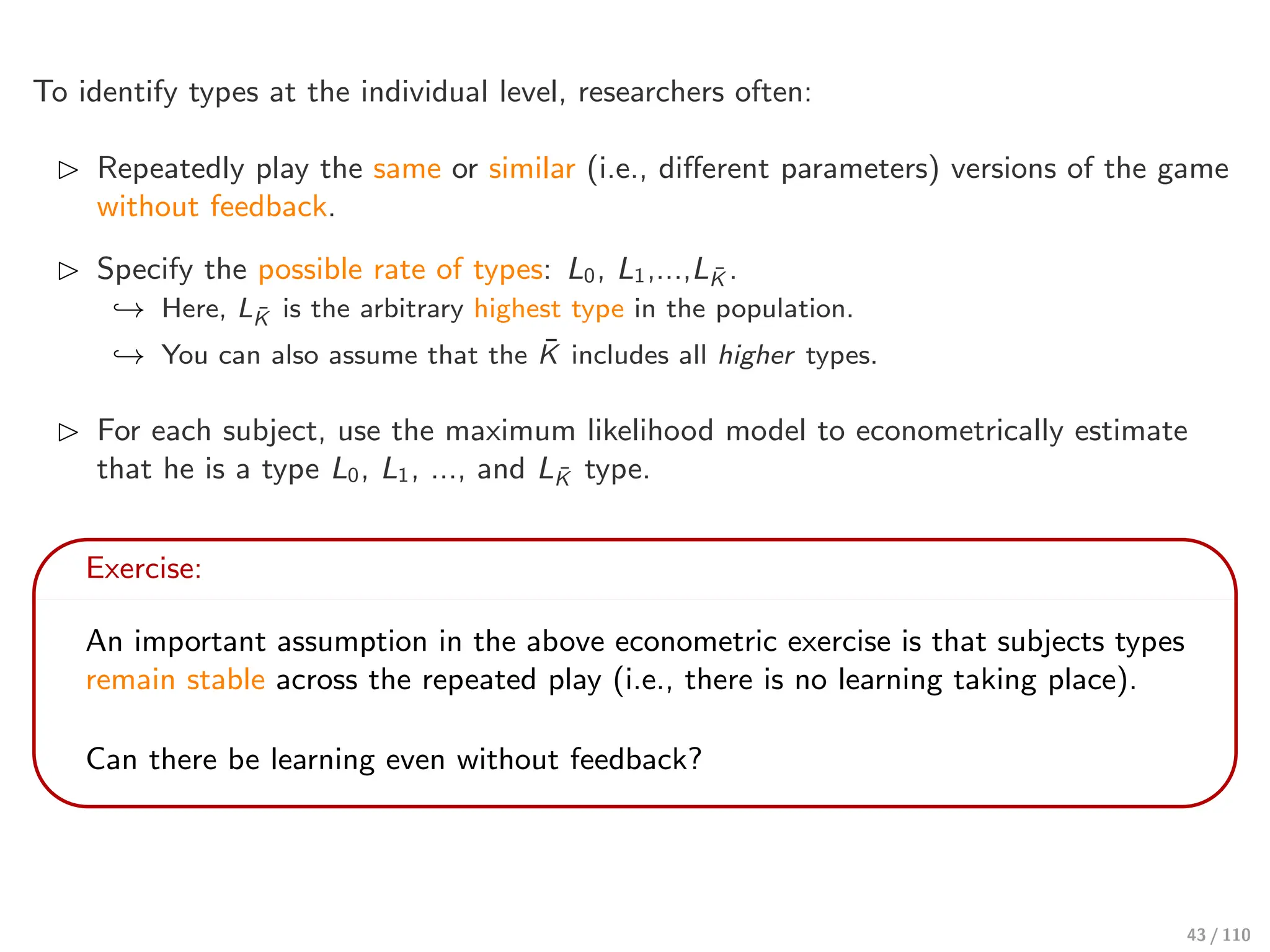
To identify typesat the individual level, researchers often:
⊲ Repeatedly play the same or similar (i.e., different parameters) versions of the game
without feedback.
⊲ Specify the possible rate of types: L0, L1,...,LK̄ .
↩→ Here, LK̄ is the arbitrary highest type in the population.
↩→ You can also assume that the K̄ includes all higher types.
⊲ For each subject, use the maximum likelihood model to econometrically estimate
that he is a type L0, L1, ..., and LK̄ type.
Exercise:
An important assumption in the above econometric exercise is that subjects types
remain stable across the repeated play (i.e., there is no learning taking place).
Can there be learning even without feedback?
43 / 110
44.
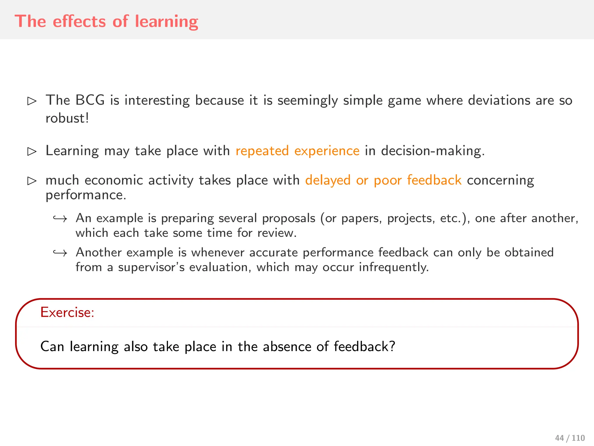
The effects oflearning
⊲ The BCG is interesting because it is seemingly simple game where deviations are so
robust!
⊲ Learning may take place with repeated experience in decision-making.
⊲ much economic activity takes place with delayed or poor feedback concerning
performance.
↩→ An example is preparing several proposals (or papers, projects, etc.), one after another,
which each take some time for review.
↩→ Another example is whenever accurate performance feedback can only be obtained
from a supervisor’s evaluation, which may occur infrequently.
Exercise:
Can learning also take place in the absence of feedback?
44 / 110
45.
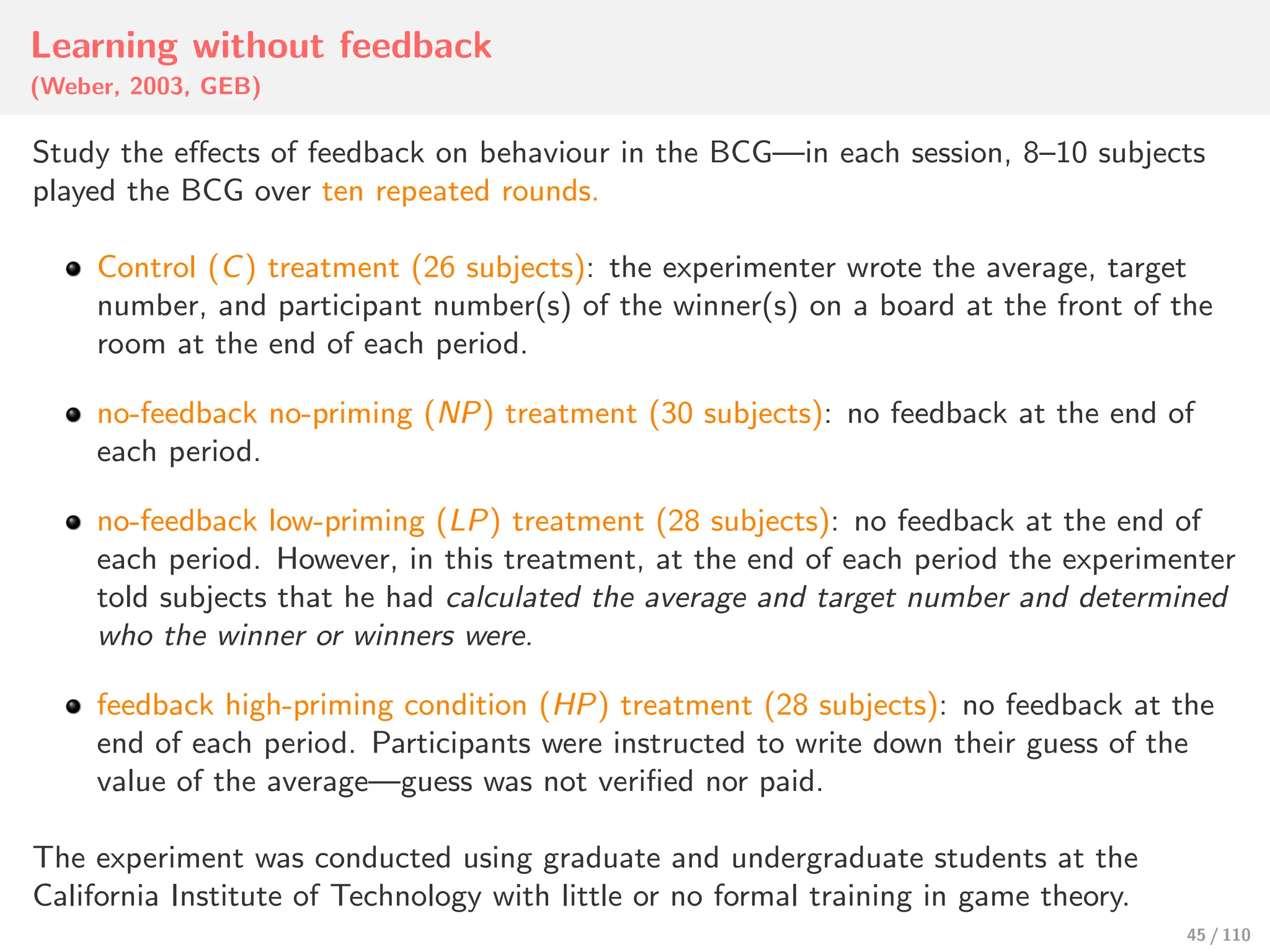
Learning without feedback
(Weber,2003, GEB)
Study the effects of feedback on behaviour in the BCG—in each session, 8–10 subjects
played the BCG over ten repeated rounds.
Control (C) treatment (26 subjects): the experimenter wrote the average, target
number, and participant number(s) of the winner(s) on a board at the front of the
room at the end of each period.
no-feedback no-priming (NP) treatment (30 subjects): no feedback at the end of
each period.
no-feedback low-priming (LP) treatment (28 subjects): no feedback at the end of
each period. However, in this treatment, at the end of each period the experimenter
told subjects that he had calculated the average and target number and determined
who the winner or winners were.
feedback high-priming condition (HP) treatment (28 subjects): no feedback at the
end of each period. Participants were instructed to write down their guess of the
value of the average—guess was not verified nor paid.
The experiment was conducted using graduate and undergraduate students at the
California Institute of Technology with little or no formal training in game theory.
45 / 110
46.
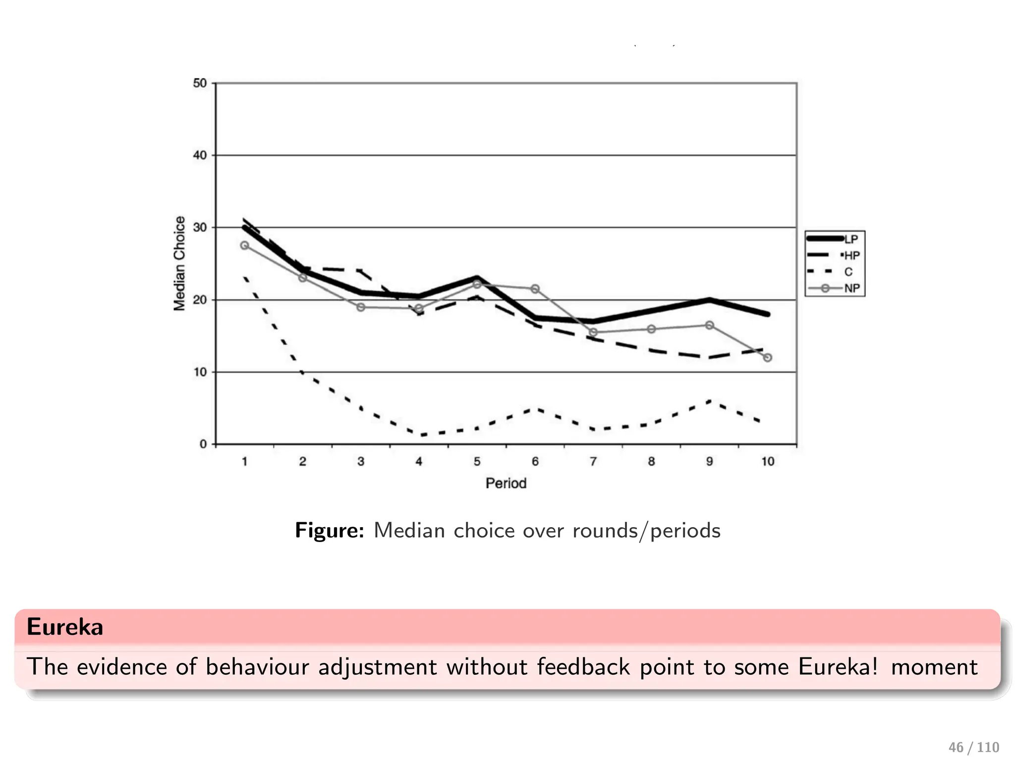
Figure: Median choiceover rounds/periods
Eureka
The evidence of behaviour adjustment without feedback point to some Eureka! moment
46 / 110
47.
Individual subject typeswithout econometric
(Choo, Kaplan and Zhou, 2019)
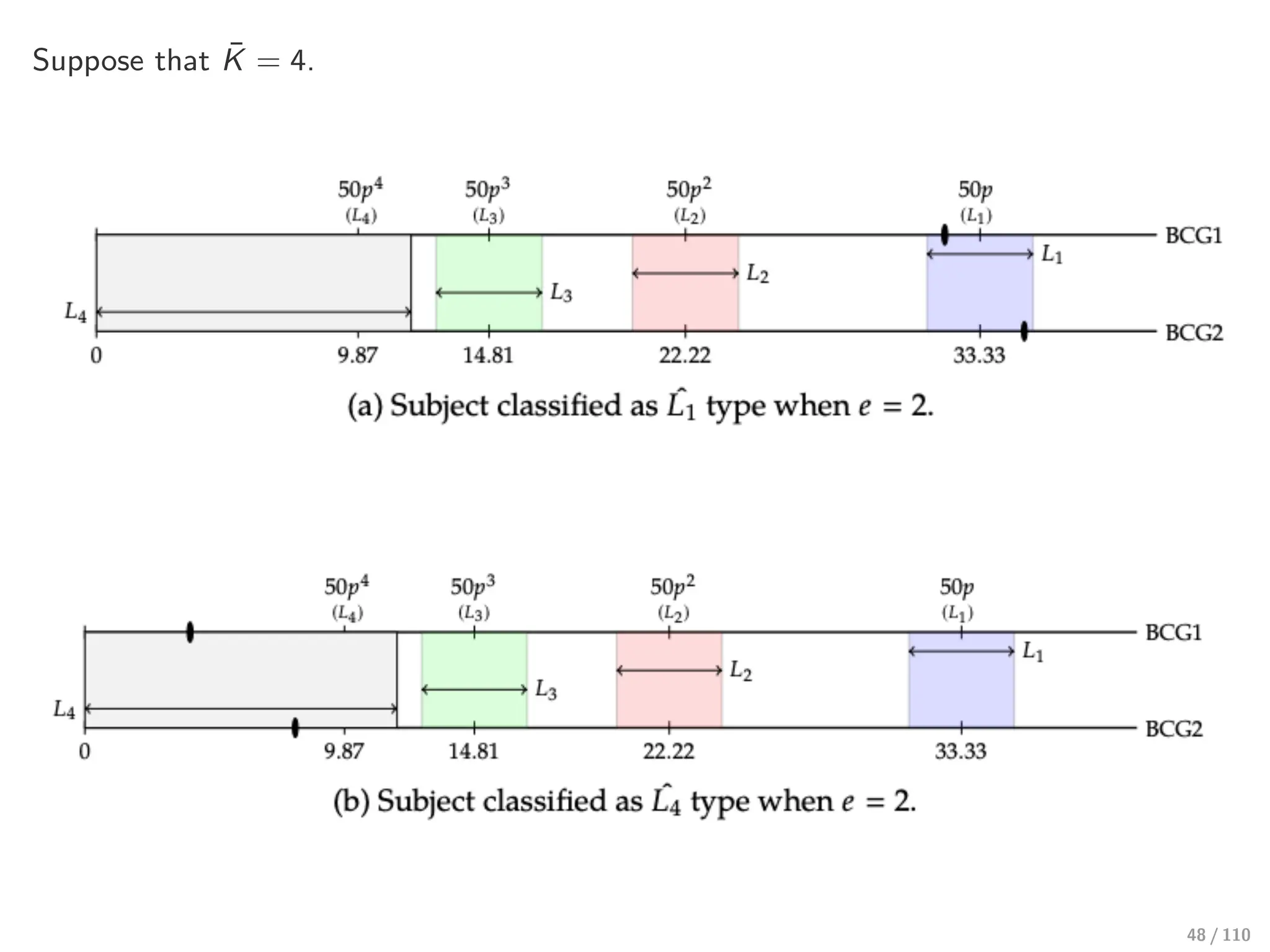
⊲ Suppose that each subject plays the n = 8 BCG twice without feedback—let BCG1
and BCG2 be their choices in the first and second BCG, respectively.
⊲ By assumption, BCG1 and BCG2 will be random for the L0 type.
⊲ Whilst each Lk (k > 0) type might pick slightly different BCG1 and BCG2 numbers,
both numbers will be close to the same predicted Lk type number (i.e., 50pk
).
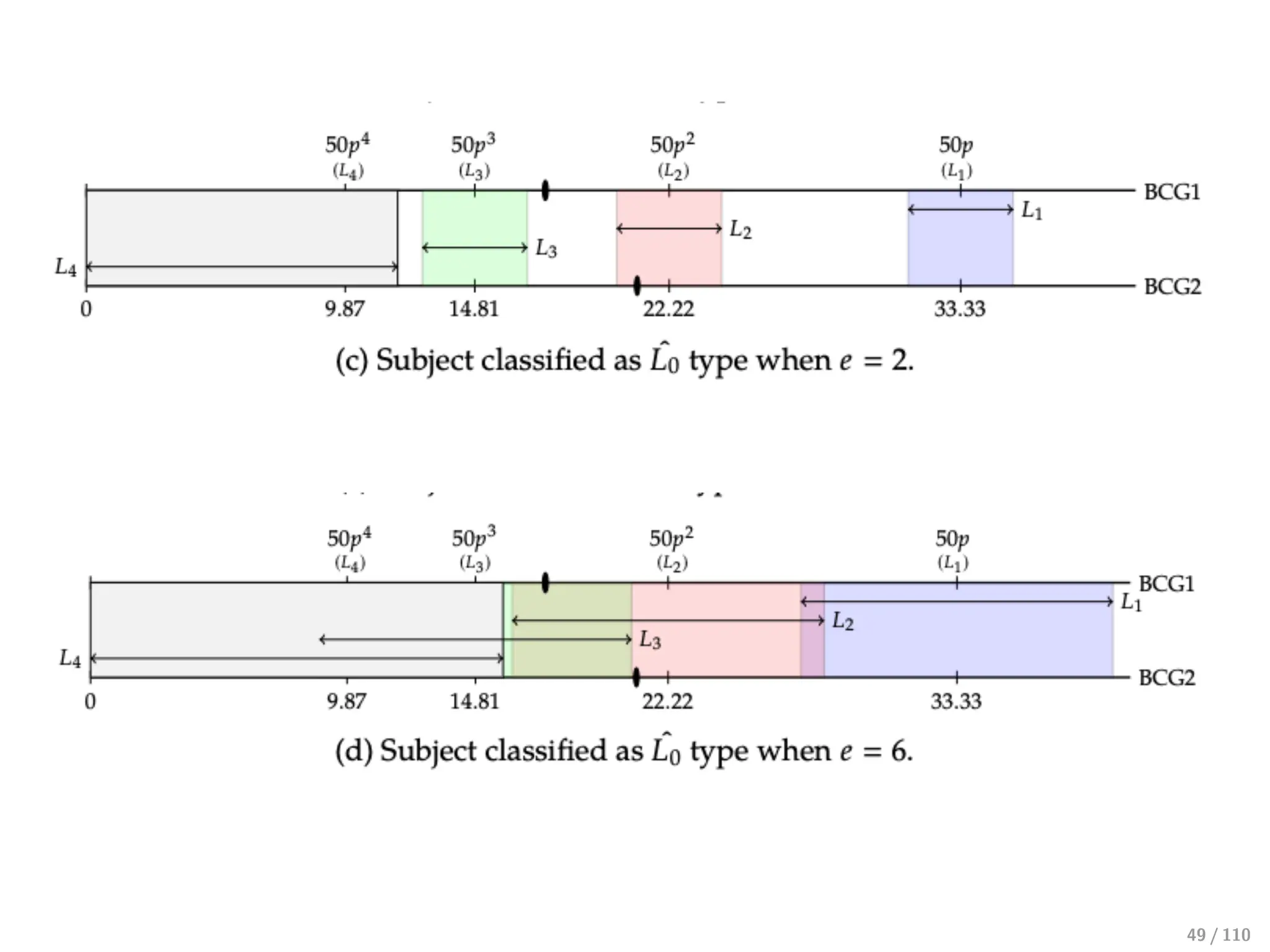
⊲ We construct a tolerance bandwidth for each Lk (k = 1, 2, ..., K̄) type—the
bandwidth around the predicted choice of each type.
↩→ L1 type bandwidth: [50p − e, 50p + e]
↩→ L2 type bandwidth: [50p2 − e, 50p2 + e]
↩→ ...
↩→ LK̄ type bandwidth: [0, 50pK̄ + e]
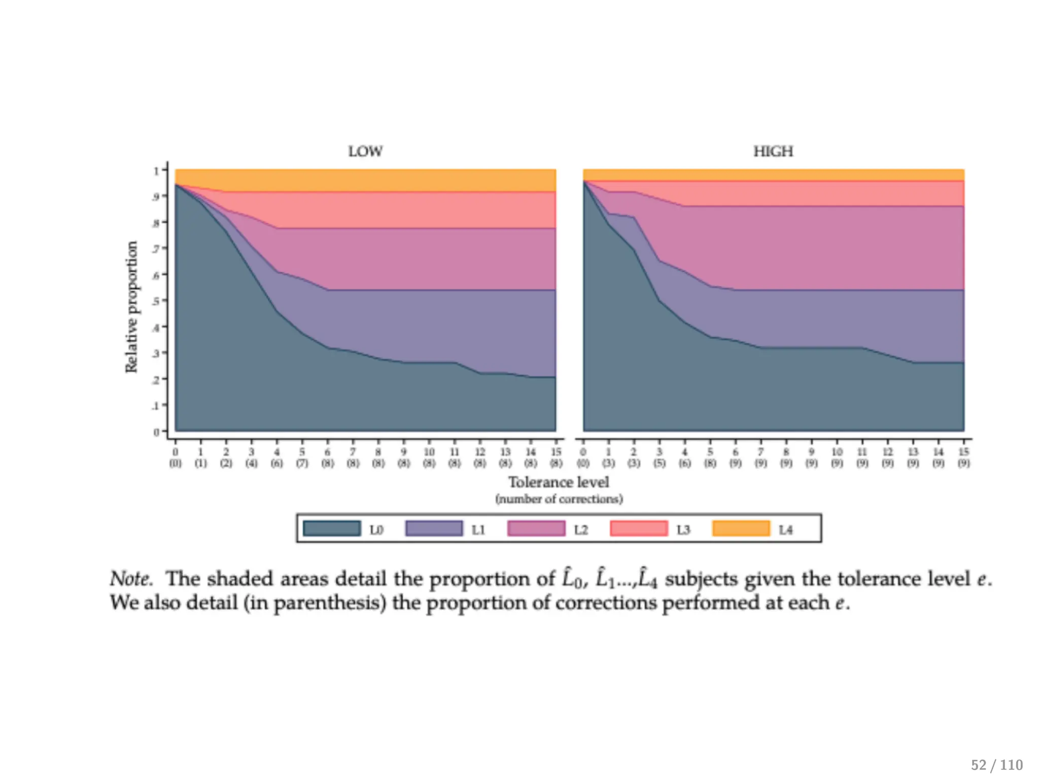
⊲ A subject is classified as type ˆ
Lk (k > 0) if both his BCG1 and BCG2 are within the
tolerance bandwidth of the Lk type—or otherwise a ˆ
L0 type.
Exercise:
How would you interpret the ˆ
L0 type?
47 / 110
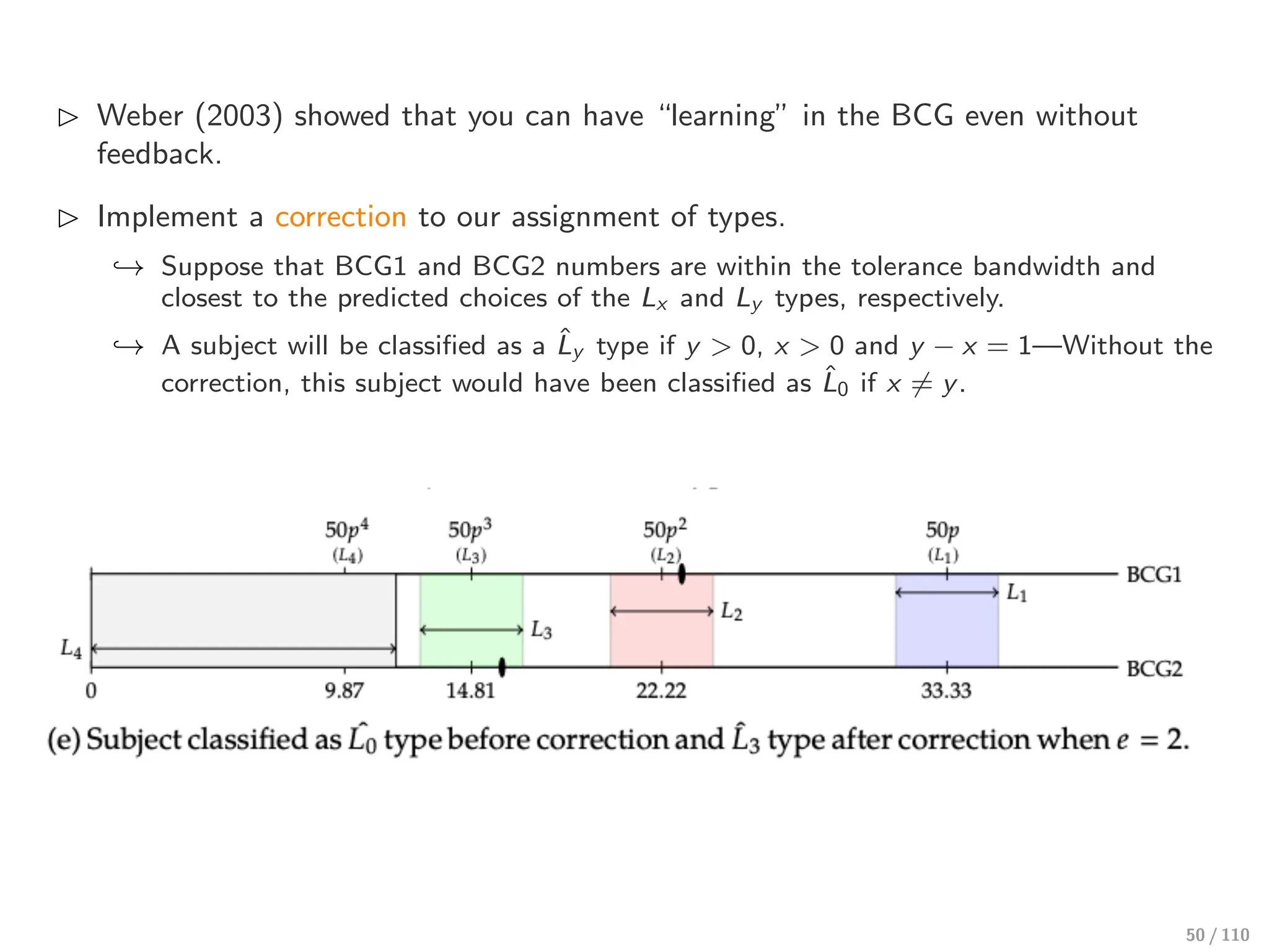
⊲ Weber (2003)showed that you can have “learning” in the BCG even without
feedback.
⊲ Implement a correction to our assignment of types.
↩→ Suppose that BCG1 and BCG2 numbers are within the tolerance bandwidth and
closest to the predicted choices of the Lx and Ly types, respectively.
↩→ A subject will be classified as a L̂y type if y > 0, x > 0 and y − x = 1—Without the
correction, this subject would have been classified as L̂0 if x ∕= y.
50 / 110
51.
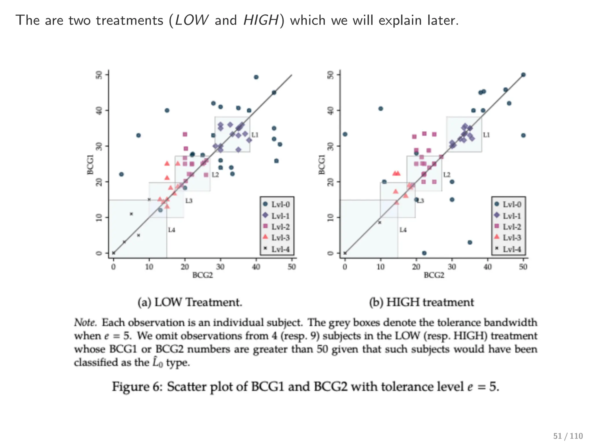
The are twotreatments (LOW and HIGH) which we will explain later.
51 / 110
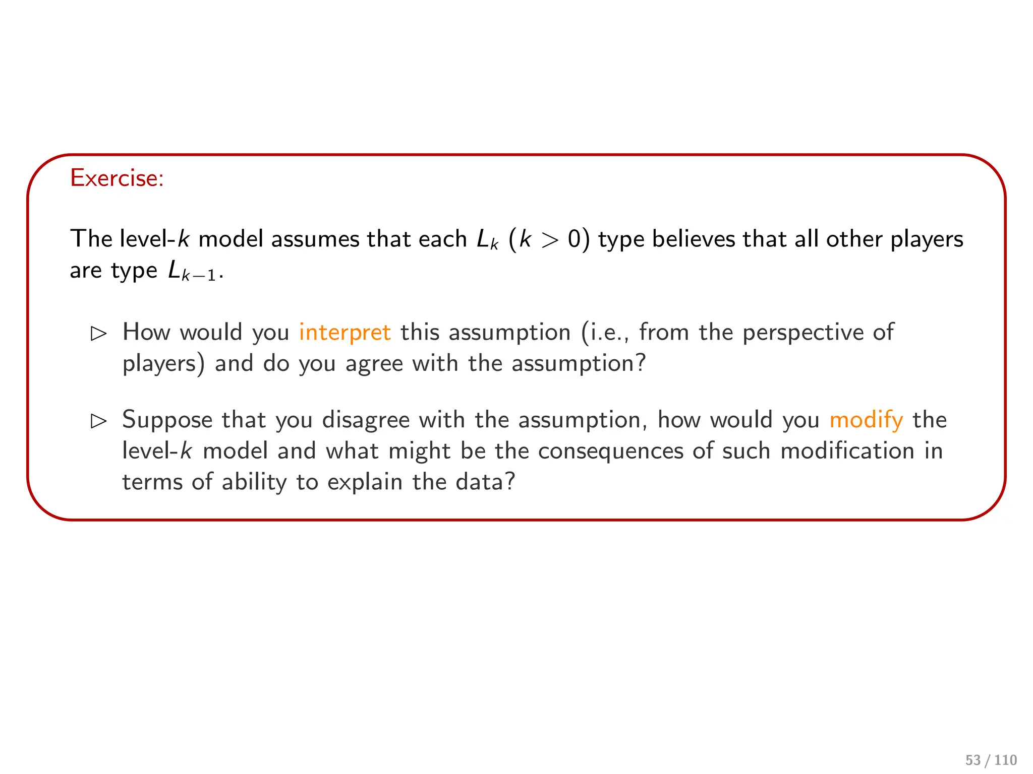
Exercise:
The level-k modelassumes that each Lk (k > 0) type believes that all other players
are type Lk−1.
⊲ How would you interpret this assumption (i.e., from the perspective of
players) and do you agree with the assumption?
⊲ Suppose that you disagree with the assumption, how would you modify the
level-k model and what might be the consequences of such modification in
terms of ability to explain the data?
53 / 110
54.
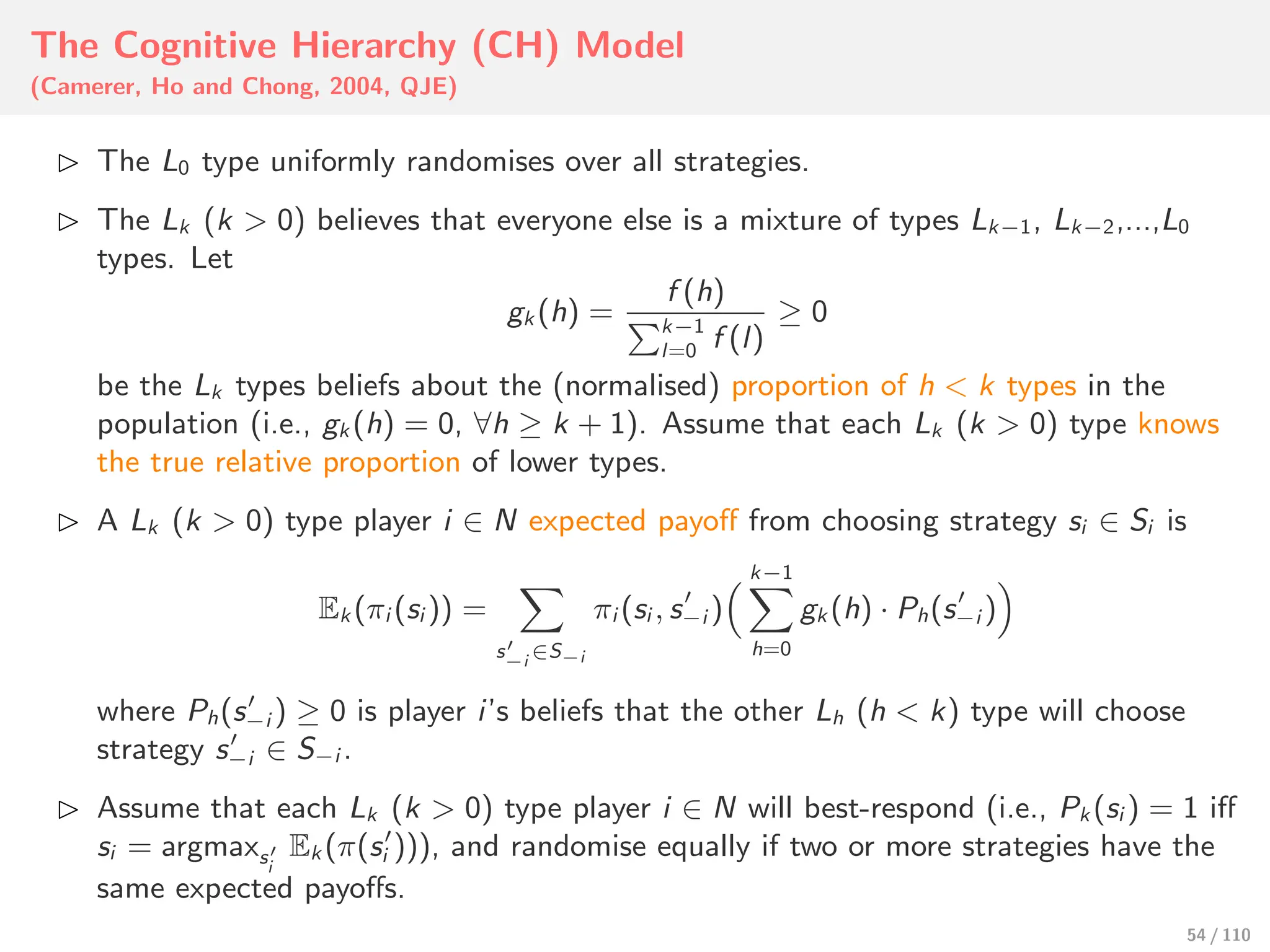
The Cognitive Hierarchy(CH) Model
(Camerer, Ho and Chong, 2004, QJE)
⊲ The L0 type uniformly randomises over all strategies.
⊲ The Lk (k > 0) believes that everyone else is a mixture of types Lk−1, Lk−2,...,L0
types. Let
gk (h) =
f (h)
%k−1
l=0 f (l)
≥ 0
be the Lk types beliefs about the (normalised) proportion of h < k types in the
population (i.e., gk (h) = 0, ∀h ≥ k + 1). Assume that each Lk (k > 0) type knows
the true relative proportion of lower types.
⊲ A Lk (k > 0) type player i ∈ N expected payoff from choosing strategy si ∈ Si is
Ek (πi (si )) =
&
s′
−i
∈S−i
πi (si , s′
−i )
' k−1
&
h=0
gk (h) · Ph(s′
−i )
(
where Ph(s′
−i ) ≥ 0 is player i’s beliefs that the other Lh (h < k) type will choose
strategy s′
−i ∈ S−i .
⊲ Assume that each Lk (k > 0) type player i ∈ N will best-respond (i.e., Pk (si ) = 1 iff
si = argmaxs′
i
Ek (π(s′
i ))), and randomise equally if two or more strategies have the
same expected payoffs.
54 / 110
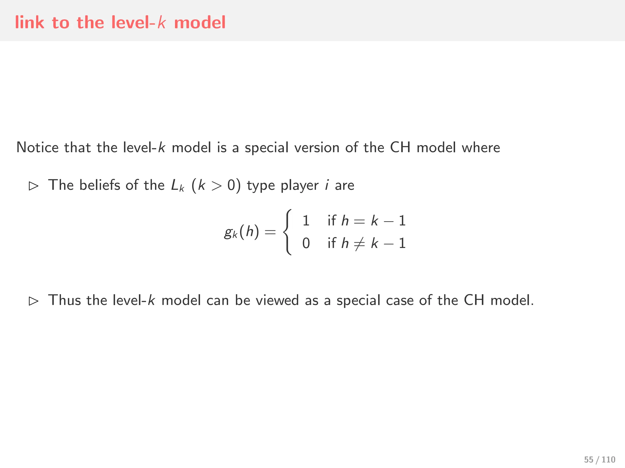
55.
link to thelevel-k model
Notice that the level-k model is a special version of the CH model where
⊲ The beliefs of the Lk (k > 0) type player i are
gk (h) =
)
1
0
if h = k − 1
if h ∕= k − 1
⊲ Thus the level-k model can be viewed as a special case of the CH model.
55 / 110
56.
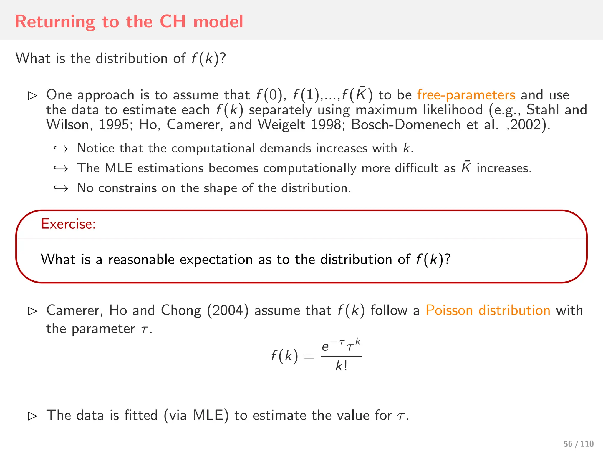
Returning to theCH model
What is the distribution of f (k)?
⊲ One approach is to assume that f (0), f (1),...,f (K̄) to be free-parameters and use
the data to estimate each f (k) separately using maximum likelihood (e.g., Stahl and
Wilson, 1995; Ho, Camerer, and Weigelt 1998; Bosch-Domenech et al. ,2002).
↩→ Notice that the computational demands increases with k.
↩→ The MLE estimations becomes computationally more difficult as K̄ increases.
↩→ No constrains on the shape of the distribution.
Exercise:
What is a reasonable expectation as to the distribution of f (k)?
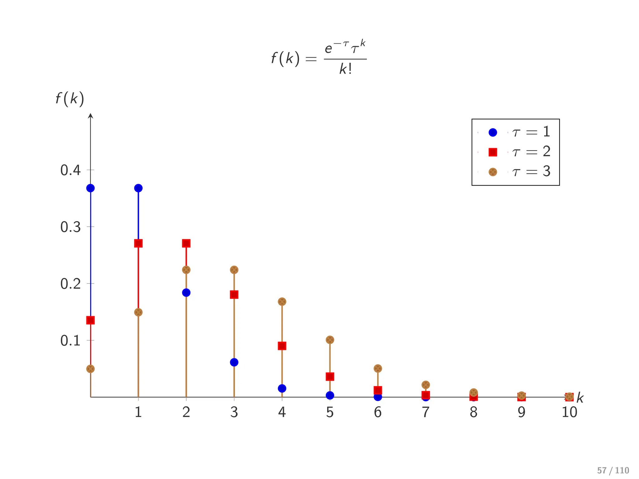
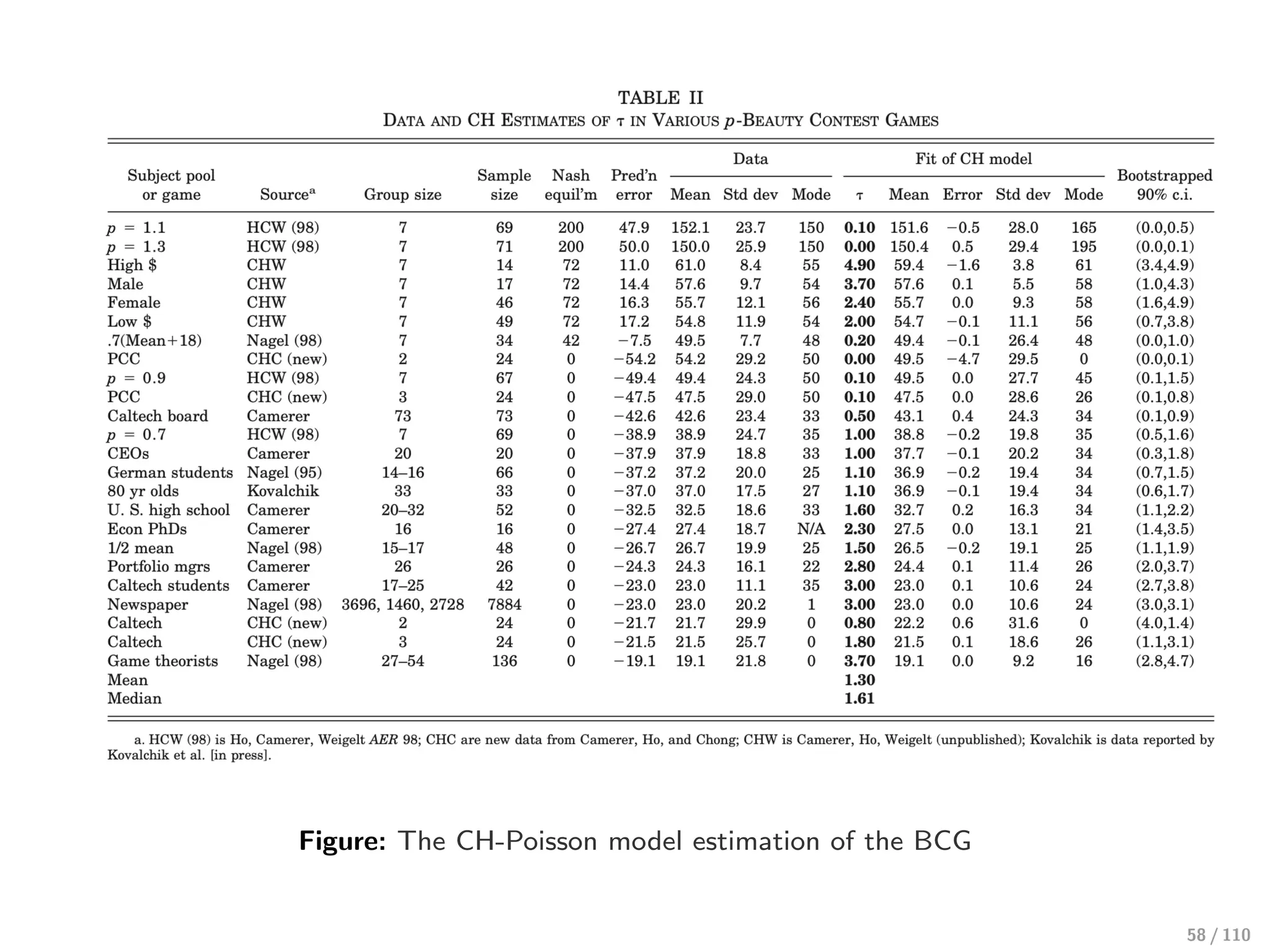
⊲ Camerer, Ho and Chong (2004) assume that f (k) follow a Poisson distribution with
the parameter τ.
f (k) =
e−τ
τk
k!
⊲ The data is fitted (via MLE) to estimate the value for τ.
56 / 110
4. Other applicationsof the level-k model
59 / 110
Basic level - 1
20 4 Le La
<:believea action = BR) Lo behavior
non shortogic
uniform randomise
choose same ↳
-
believe, an action =
BRC4 behar)
action
it
L
60.
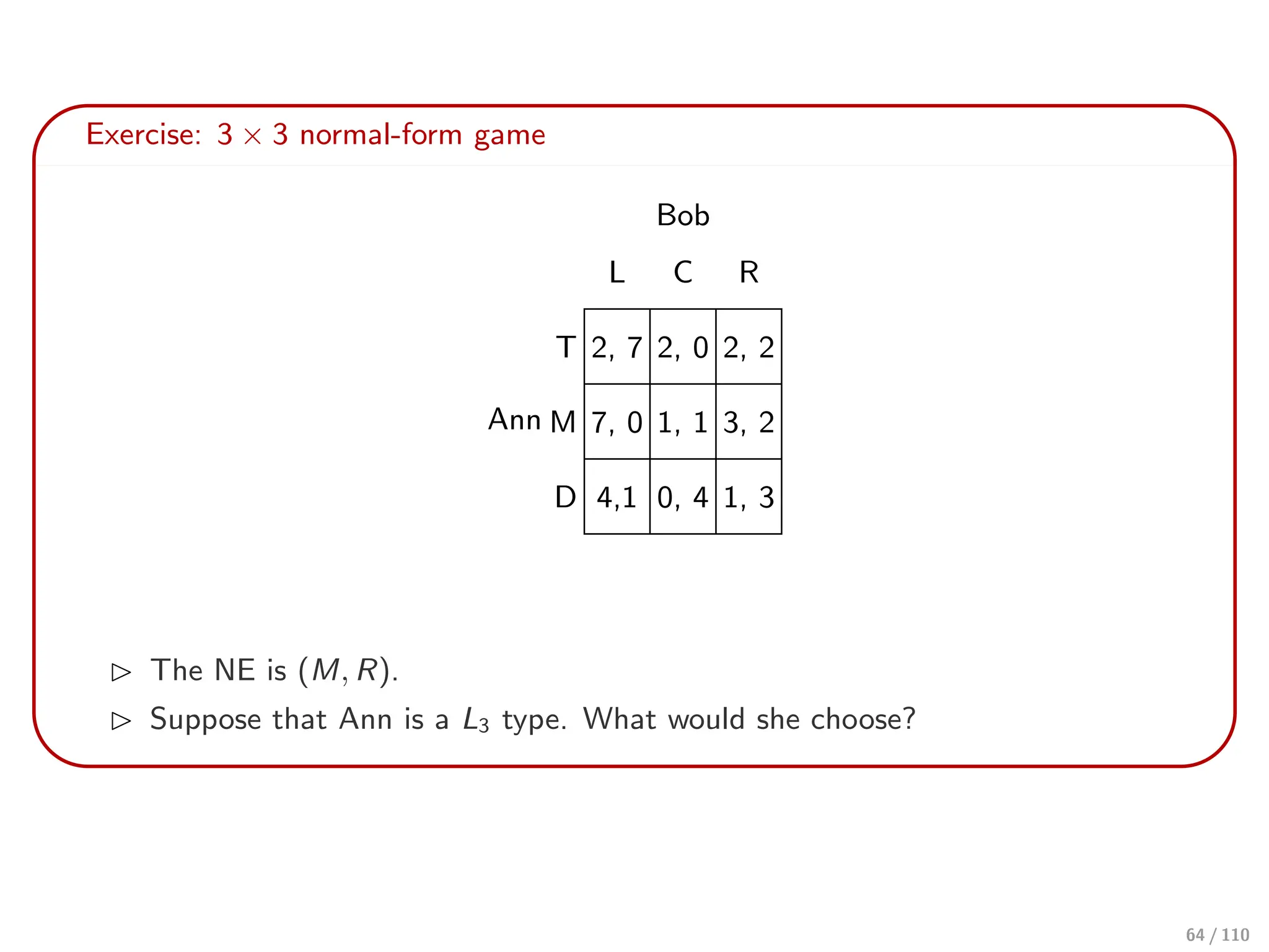
Exercise: 3 ×3 normal-form game
Ann
Bob
L C R
T 2, 7 2, 0 2, 2
M 7, 0 1, 1 3, 2
D 4,1 0, 4 1, 3
⊲ The NE is (M, R).
⊲ Suppose that Ann is a L1 type. What would she choose?
60 / 110
61.
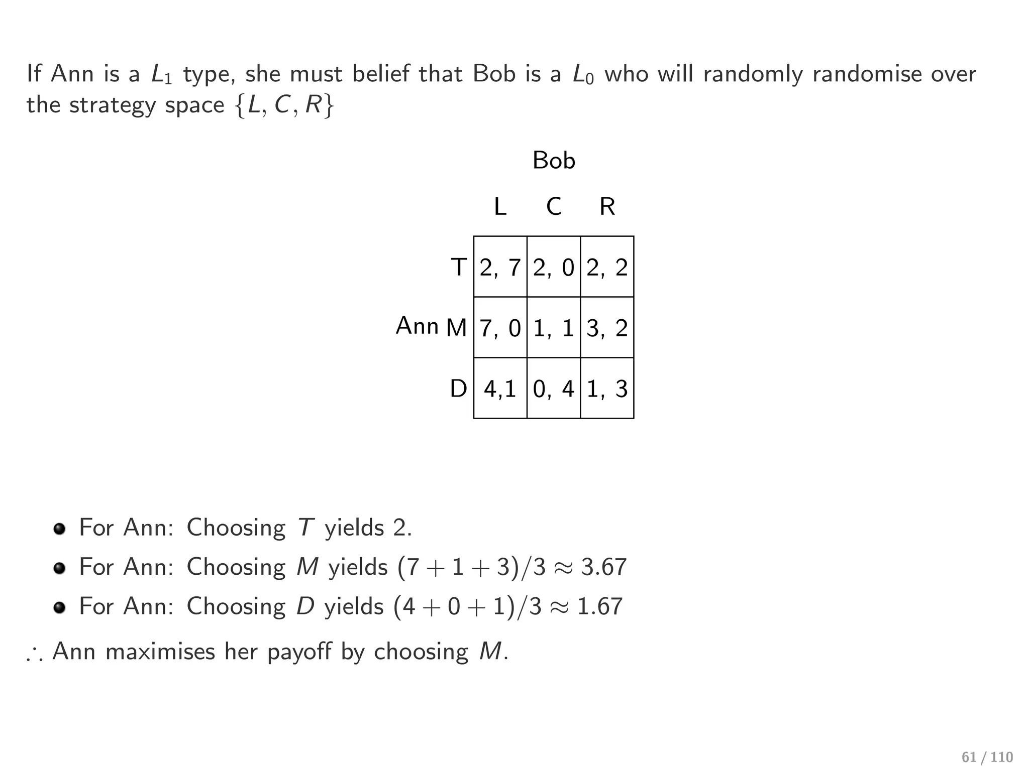
If Ann isa L1 type, she must belief that Bob is a L0 who will randomly randomise over
the strategy space {L, C, R}
Ann
Bob
L C R
T 2, 7 2, 0 2, 2
M 7, 0 1, 1 3, 2
D 4,1 0, 4 1, 3
For Ann: Choosing T yields 2.
For Ann: Choosing M yields (7 + 1 + 3)/3 ≈ 3.67
For Ann: Choosing D yields (4 + 0 + 1)/3 ≈ 1.67
∴ Ann maximises her payoff by choosing M.
61 / 110
62.
Exercise: 3 ×3 normal-form game
Ann
Bob
L C R
T 2, 7 2, 0 2, 2
M 7, 0 1, 1 3, 2
D 4,1 0, 4 1, 3
⊲ The NE is (M, R).
⊲ Suppose that Ann is a L2 type. What would she choose?
62 / 110
63.
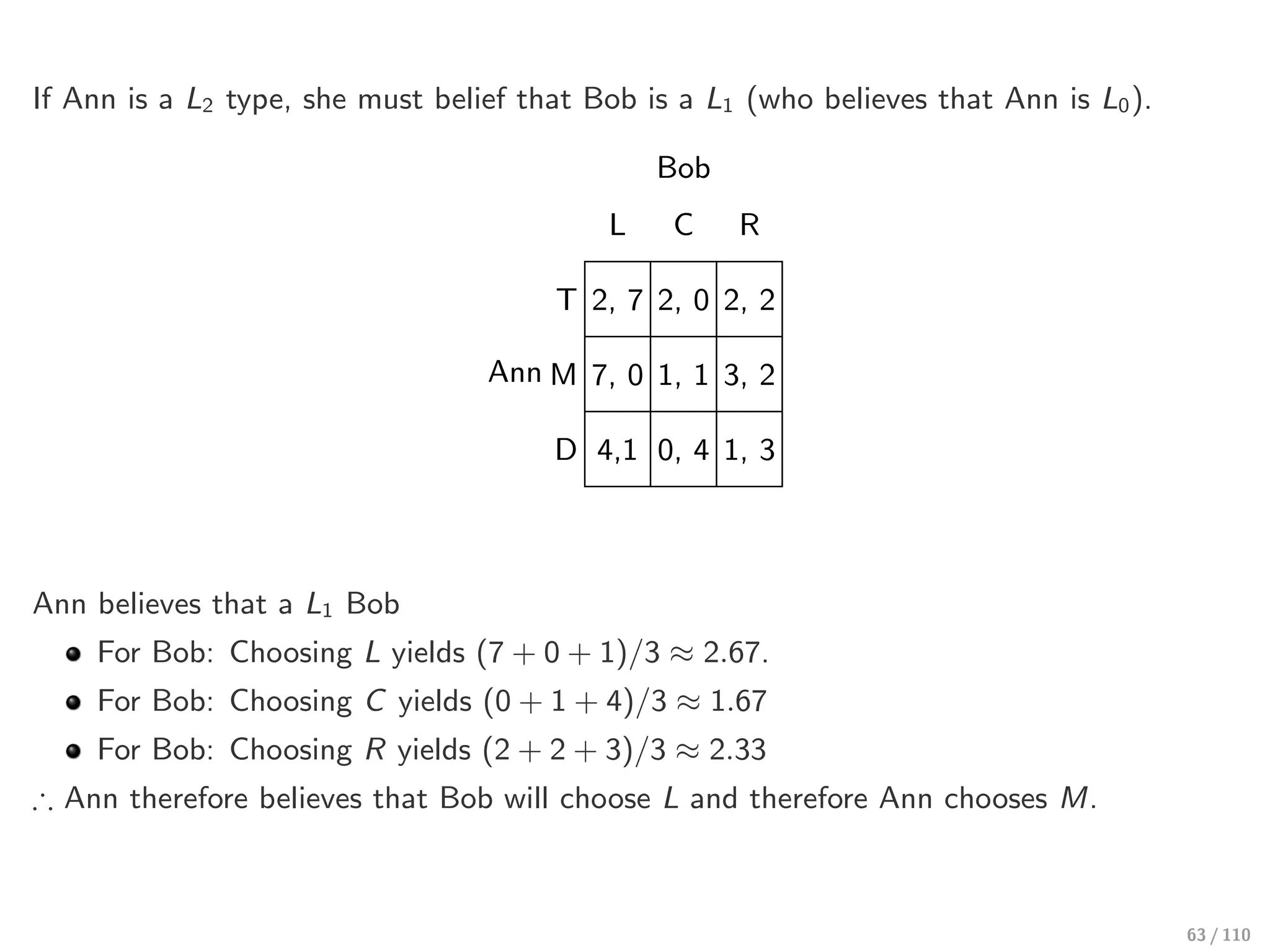
If Ann isa L2 type, she must belief that Bob is a L1 (who believes that Ann is L0).
Ann
Bob
L C R
T 2, 7 2, 0 2, 2
M 7, 0 1, 1 3, 2
D 4,1 0, 4 1, 3
Ann believes that a L1 Bob
For Bob: Choosing L yields (7 + 0 + 1)/3 ≈ 2.67.
For Bob: Choosing C yields (0 + 1 + 4)/3 ≈ 1.67
For Bob: Choosing R yields (2 + 2 + 3)/3 ≈ 2.33
∴ Ann therefore believes that Bob will choose L and therefore Ann chooses M.
63 / 110
64.
Exercise: 3 ×3 normal-form game
Ann
Bob
L C R
T 2, 7 2, 0 2, 2
M 7, 0 1, 1 3, 2
D 4,1 0, 4 1, 3
⊲ The NE is (M, R).
⊲ Suppose that Ann is a L3 type. What would she choose?
64 / 110
65.
Ann
Bob
L C R
T2, 7 2, 0 2, 2
M 7, 0 1, 1 3, 2
D 4,1 0, 4 1, 3
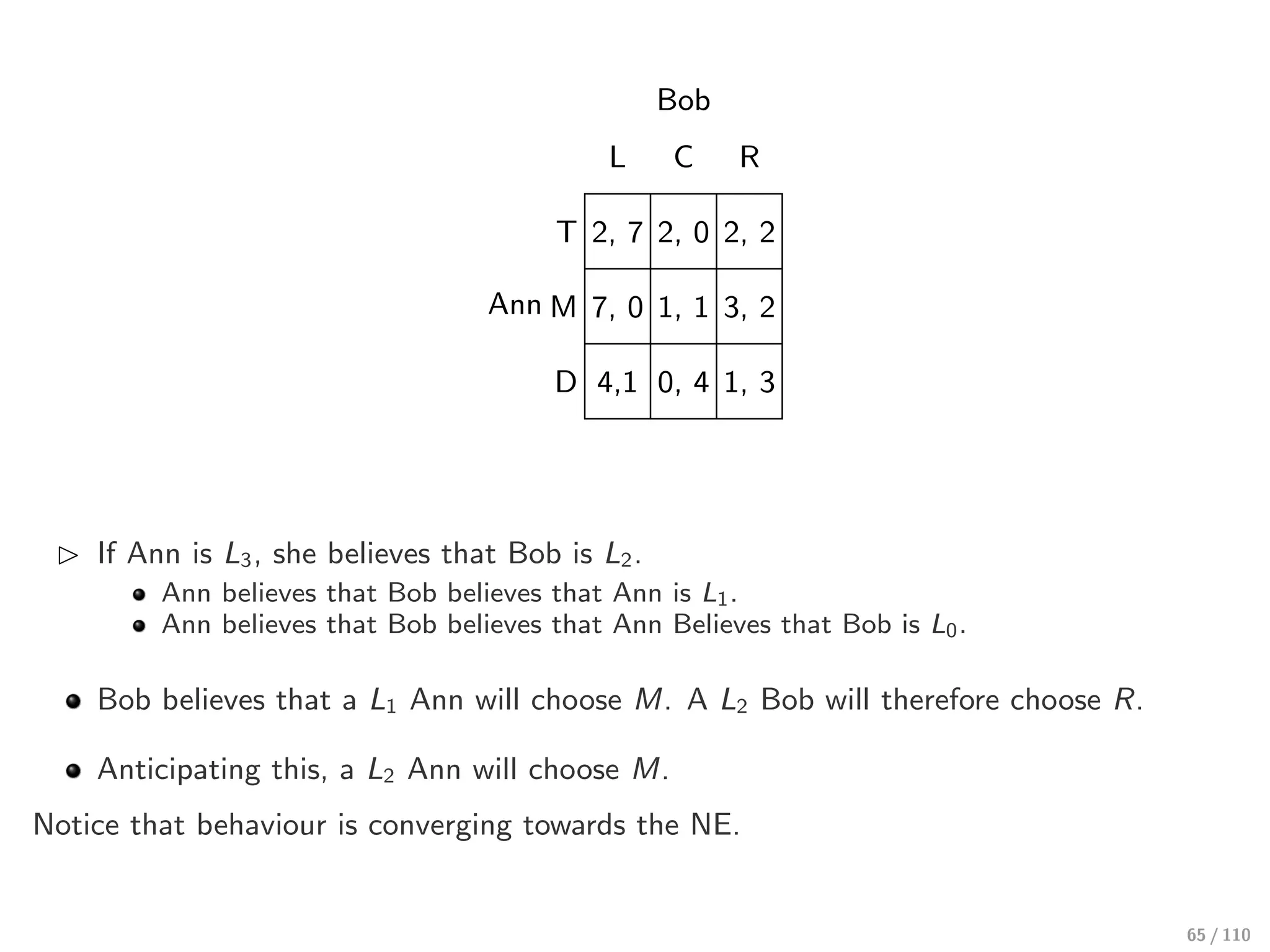
⊲ If Ann is L3, she believes that Bob is L2.
Ann believes that Bob believes that Ann is L1.
Ann believes that Bob believes that Ann Believes that Bob is L0.
Bob believes that a L1 Ann will choose M. A L2 Bob will therefore choose R.
Anticipating this, a L2 Ann will choose M.
Notice that behaviour is converging towards the NE.
65 / 110
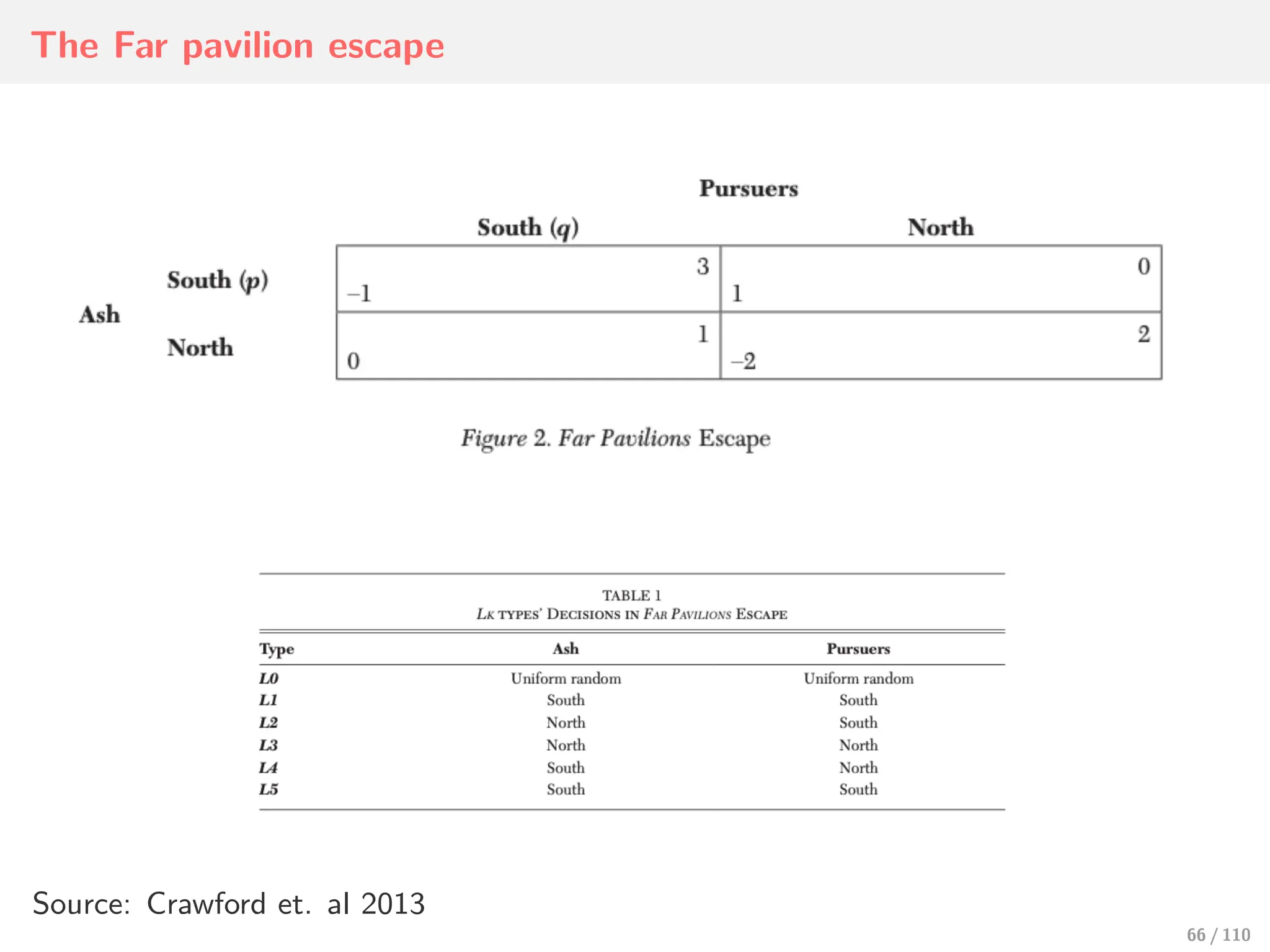
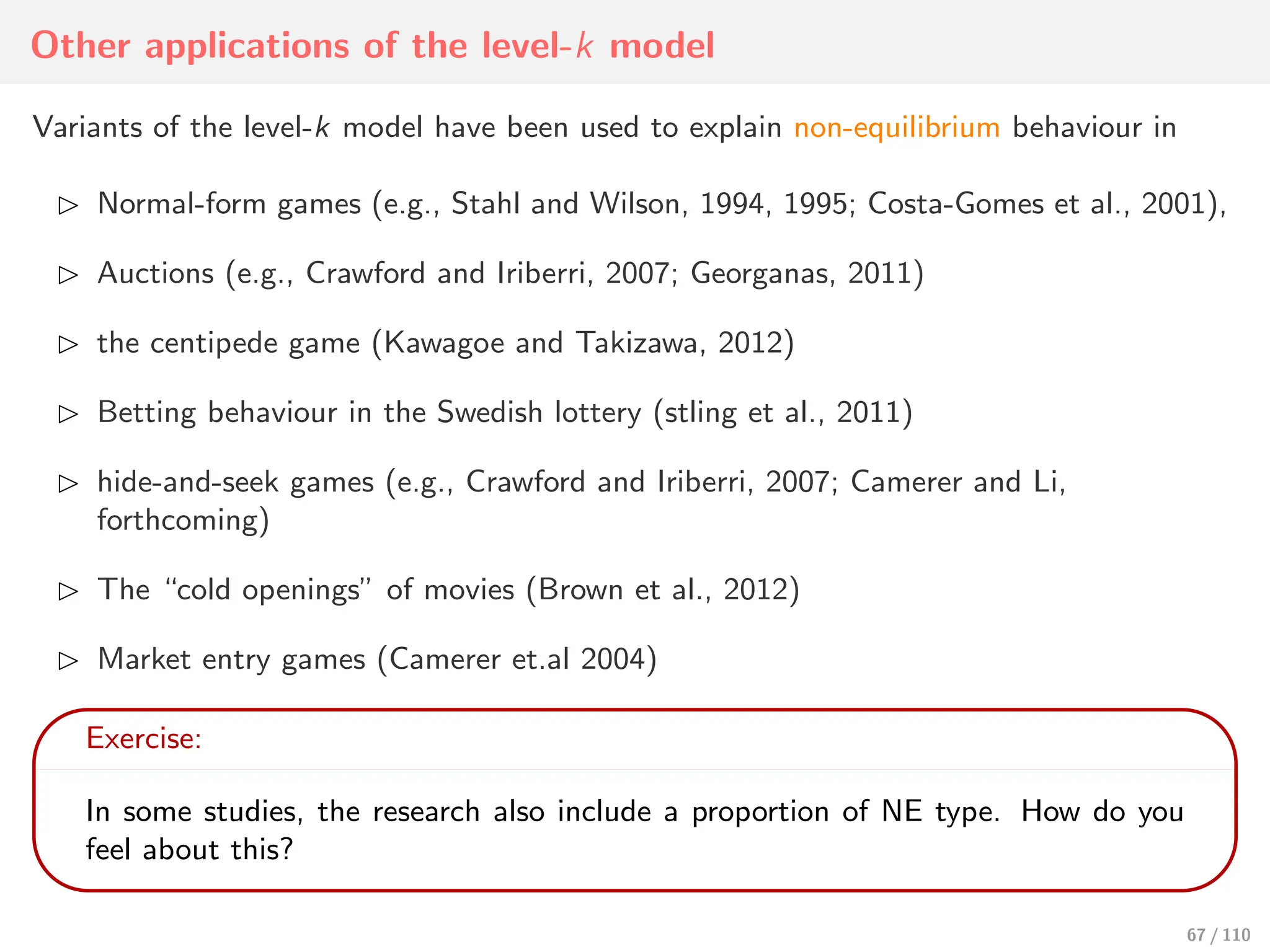
Other applications ofthe level-k model
Variants of the level-k model have been used to explain non-equilibrium behaviour in
⊲ Normal-form games (e.g., Stahl and Wilson, 1994, 1995; Costa-Gomes et al., 2001),
⊲ Auctions (e.g., Crawford and Iriberri, 2007; Georganas, 2011)
⊲ the centipede game (Kawagoe and Takizawa, 2012)
⊲ Betting behaviour in the Swedish lottery (stling et al., 2011)
⊲ hide-and-seek games (e.g., Crawford and Iriberri, 2007; Camerer and Li,
forthcoming)
⊲ The “cold openings” of movies (Brown et al., 2012)
⊲ Market entry games (Camerer et.al 2004)
Exercise:
In some studies, the research also include a proportion of NE type. How do you
feel about this?
67 / 110
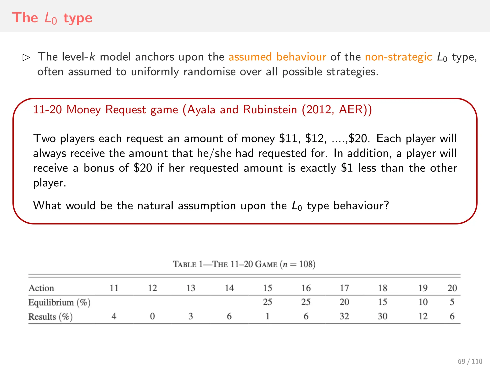
The L0 type
⊲The level-k model anchors upon the assumed behaviour of the non-strategic L0 type,
often assumed to uniformly randomise over all possible strategies.
11-20 Money Request game (Ayala and Rubinstein (2012, AER))
Two players each request an amount of money $11, $12, ....,$20. Each player will
always receive the amount that he/she had requested for. In addition, a player will
receive a bonus of $20 if her requested amount is exactly $1 less than the other
player.
What would be the natural assumption upon the L0 type behaviour?
69 / 110
70.
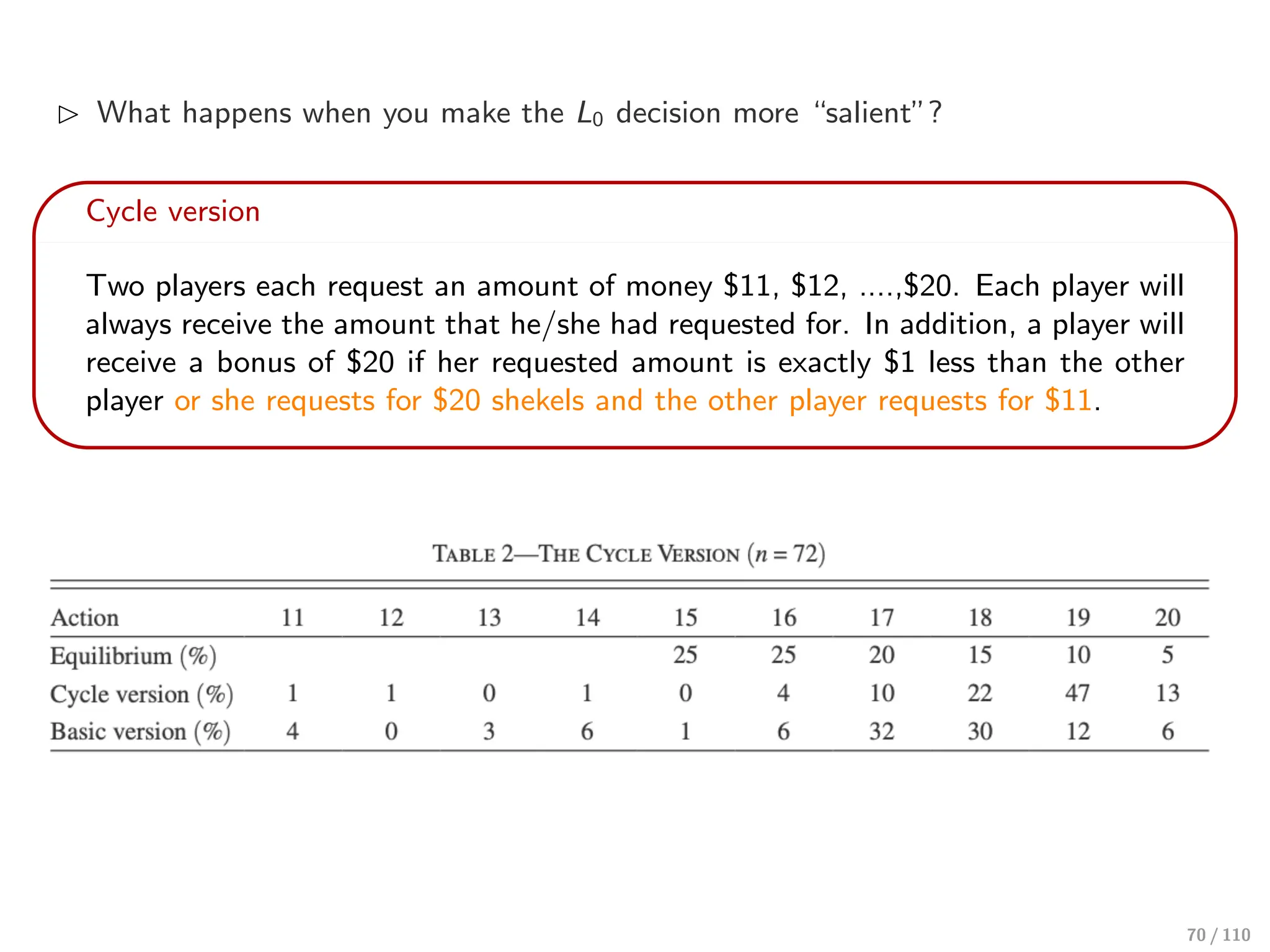
⊲ What happenswhen you make the L0 decision more “salient”?
Cycle version
Two players each request an amount of money $11, $12, ....,$20. Each player will
always receive the amount that he/she had requested for. In addition, a player will
receive a bonus of $20 if her requested amount is exactly $1 less than the other
player or she requests for $20 shekels and the other player requests for $11.
70 / 110
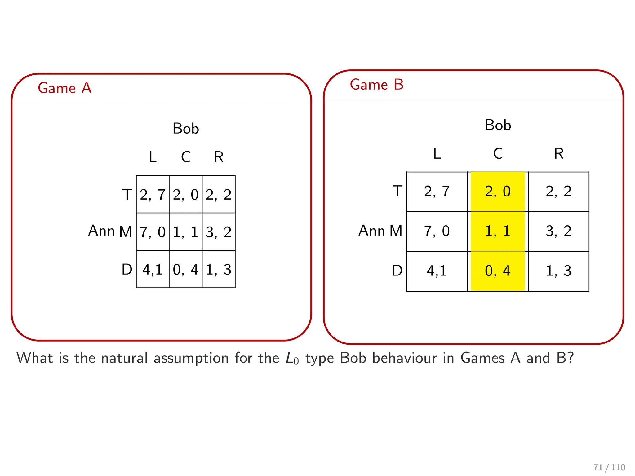
71.
Game A
Ann
Bob
L CR
T 2, 7 2, 0 2, 2
M 7, 0 1, 1 3, 2
D 4,1 0, 4 1, 3
Game B
Ann
Bob
L C R
T 2, 7 2, 0 2, 2
M 7, 0 1, 1 3, 2
D 4,1 0, 4 1, 3
What is the natural assumption for the L0 type Bob behaviour in Games A and B?
71 / 110
72.
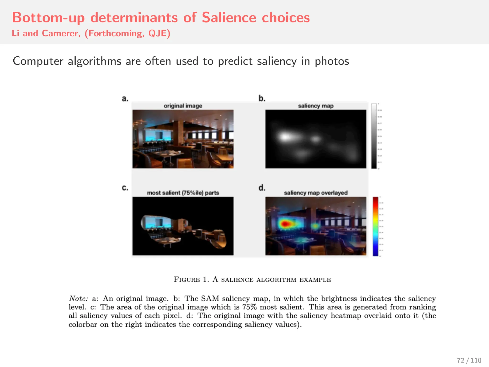
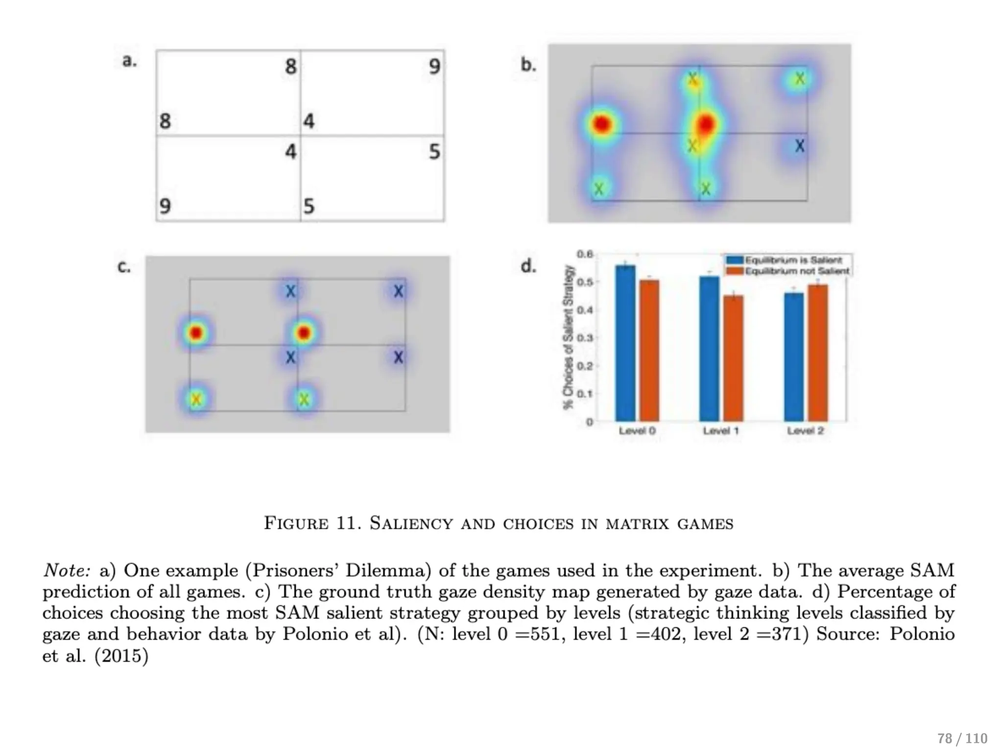
Bottom-up determinants ofSalience choices
Li and Camerer, (Forthcoming, QJE)
Computer algorithms are often used to predict saliency in photos
72 / 110
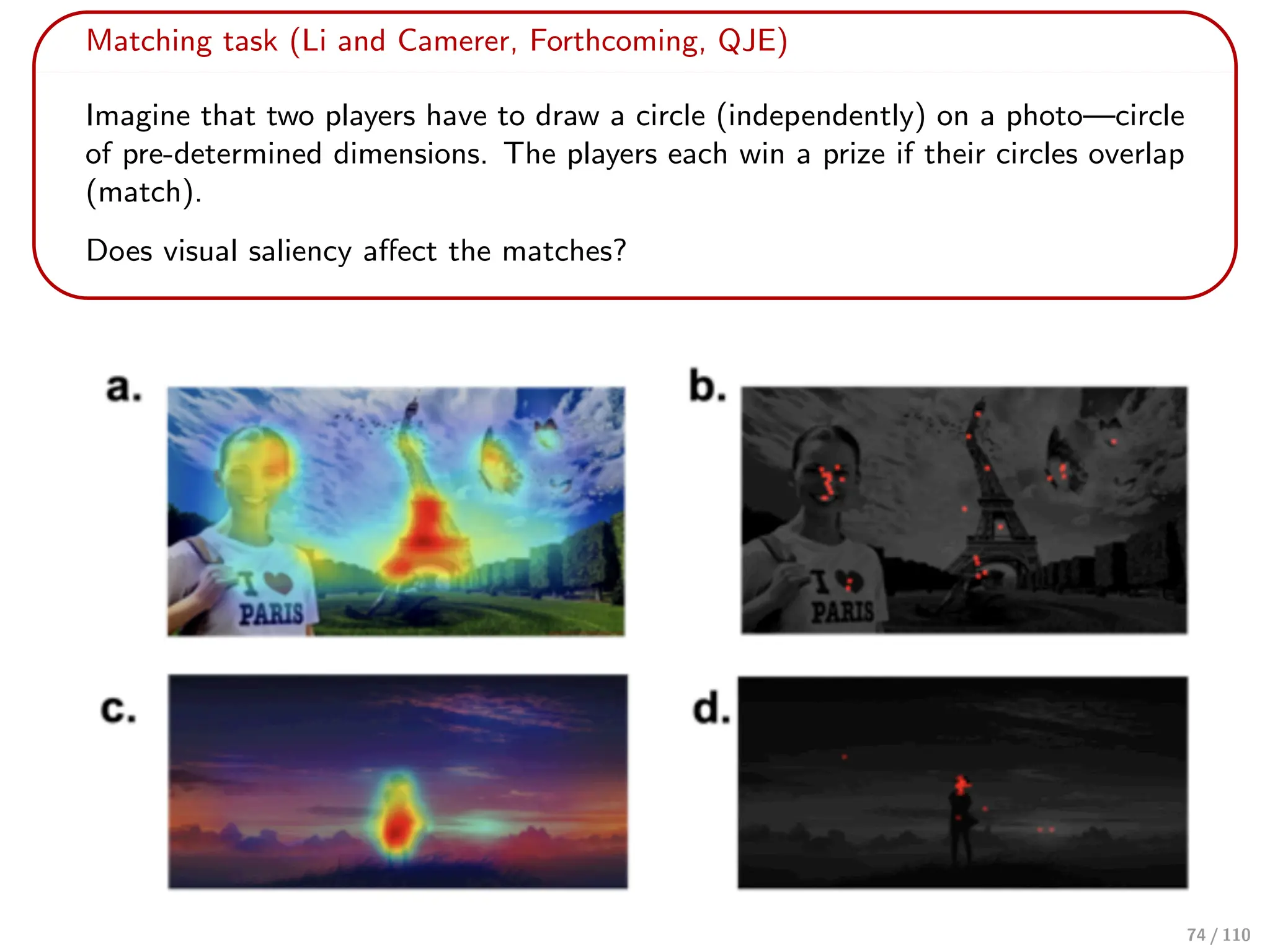
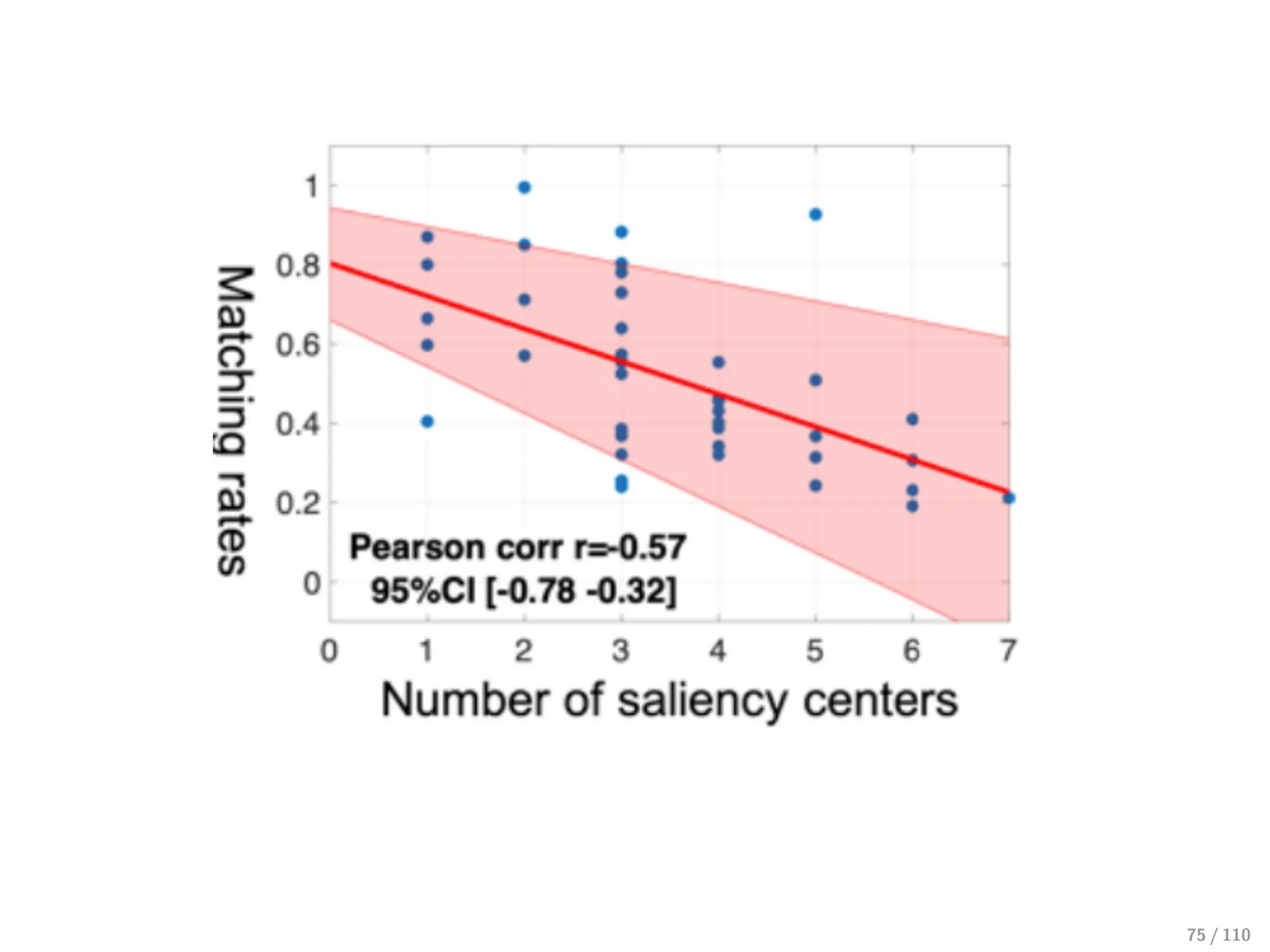
Matching task (Liand Camerer, Forthcoming, QJE)
Imagine that two players have to draw a circle (independently) on a photo—circle
of pre-determined dimensions. The players each win a prize if their circles overlap
(match).
Does visual saliency affect the matches?
74 / 110
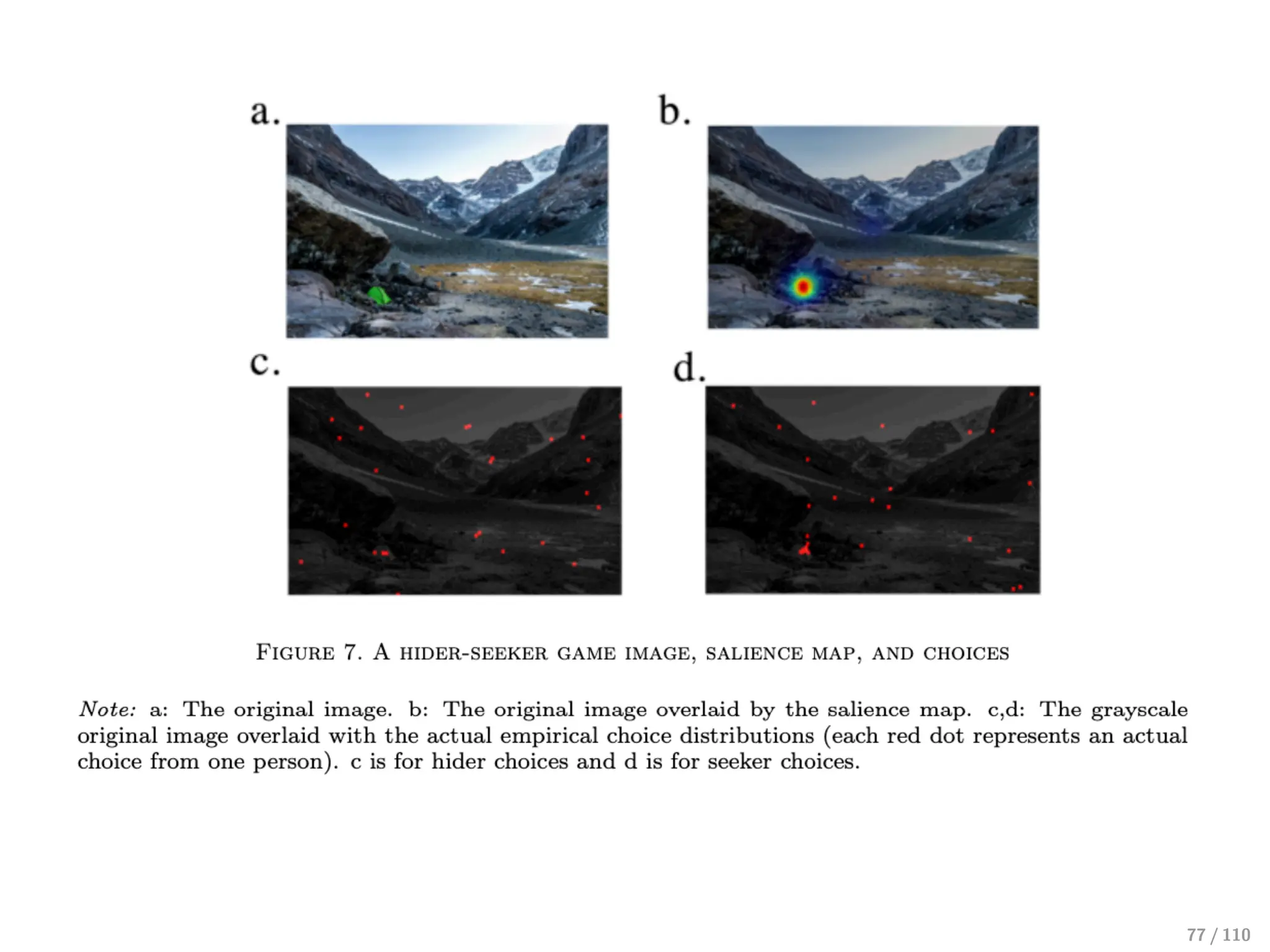
Hide-and-seek (Li andCamerer, Forthcoming, QJE)
Imagine that two players have to draw a circle (independently) on a photo—circle
of pre-determined dimensions. The “hider” earns a prize if the circles do not
overlap. In contrast, the seeker earns a prize if the circles overlap What is the
level-k model narrative of behaviour?
76 / 110
Types and Cognitiveabilities
⊲ Insofar, we have interpreted a Lk type as simply the player’s beliefs as to the
behaviour of others—types map onto a strategy.
⊲ This seems reasonable for simple games such as the 11-20 money request game
(Ayala and Rubinstein, 2012) where there are no apparent cognitive cost with doing
each additional step of thought iteration—higher types do more thought iterations.
⊲ However, with Normal-form games, and possibly also the BCG, each additional
thought iteration is accompanied by more complex payoff computations.
Exercise:
If thought iterations are cognitively costly, would higher Lk also be associated with
higher cognitive abilities?
80 / 110
81.
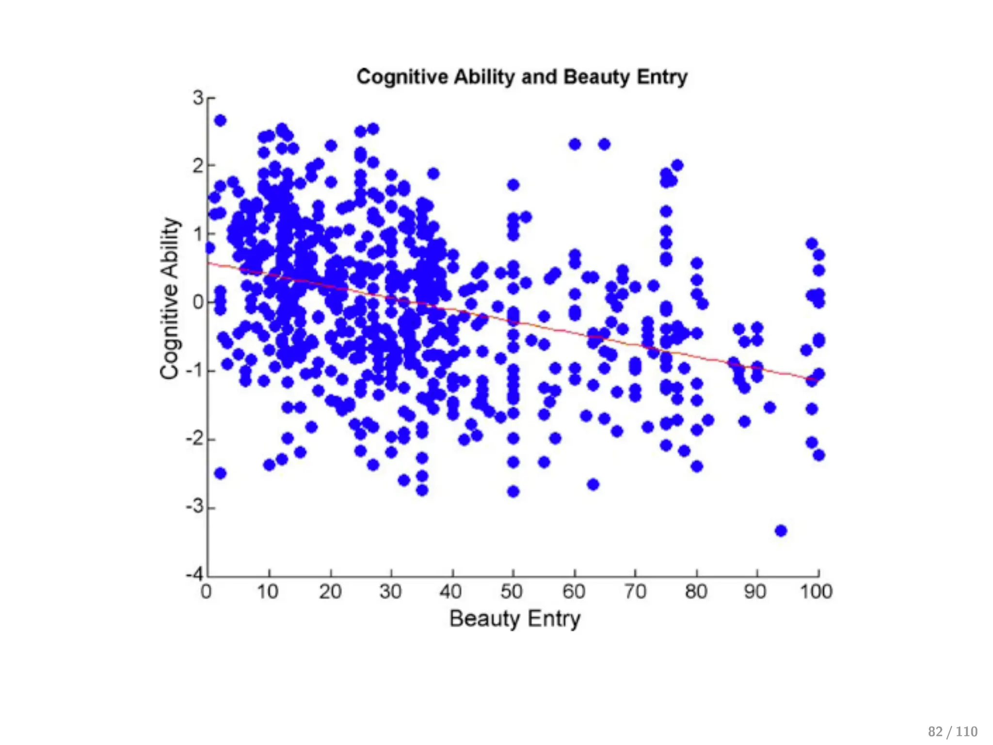
Cognitive abilities anddecisions in the BCG
(Burnham, Cesarin, Johannesson, Lichtenstein and Wallace, 2009, JEBO)
⊲ Experiment (658 subjects) embedded into a regular survey administered to a
representative group in Sweden—subjects were same sex twins.
⊲ Recruited subjects were invited to a nearby college for the experiment.
⊲ Subjects first perform a psychometric test of cognitive ability developed by the
Swedish psychometric company Assessio (Sjoberg et al., 2006).
⊲ Thereafter, subjects played the BCG (p = 0.5) game against each other (large scale
BCG) for a prize of approximately 1000 RMB (conducted in 2006).
↩→ The researchers emphasised that deception is not promoted in economics.
81 / 110
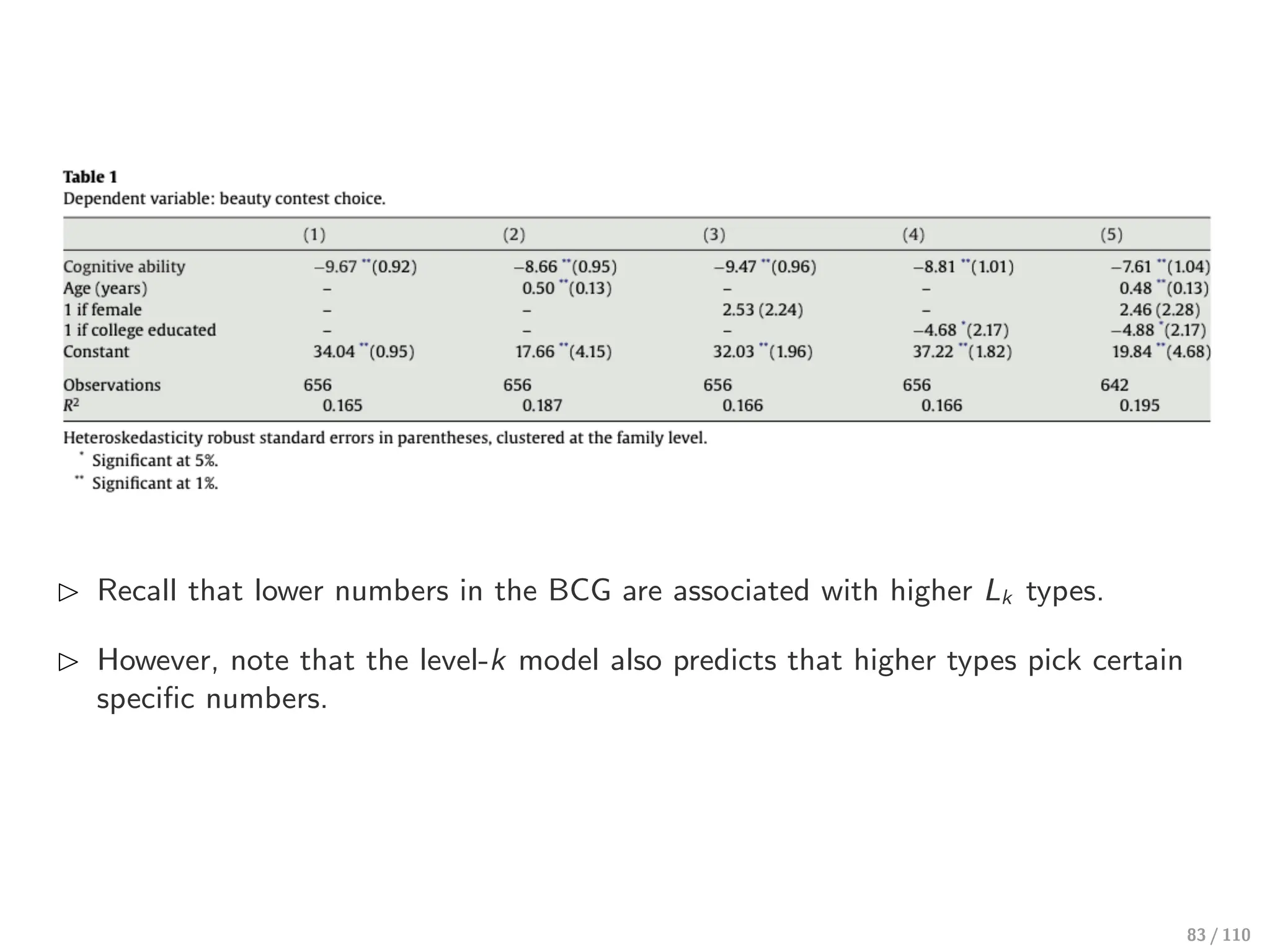
⊲ Recall thatlower numbers in the BCG are associated with higher Lk types.
⊲ However, note that the level-k model also predicts that higher types pick certain
specific numbers.
83 / 110
84.
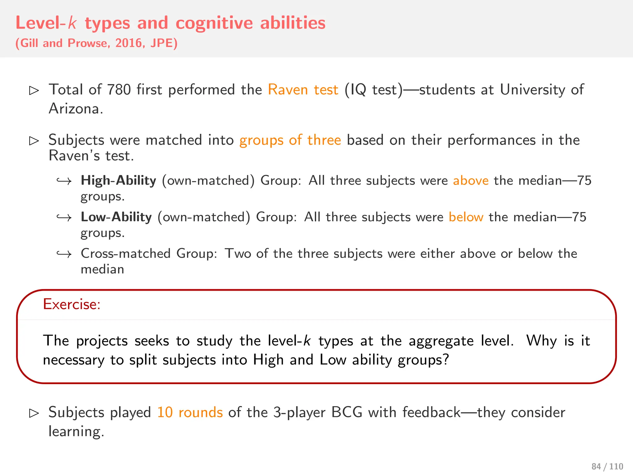
Level-k types andcognitive abilities
(Gill and Prowse, 2016, JPE)
⊲ Total of 780 first performed the Raven test (IQ test)—students at University of
Arizona.
⊲ Subjects were matched into groups of three based on their performances in the
Raven’s test.
↩→ High-Ability (own-matched) Group: All three subjects were above the median—75
groups.
↩→ Low-Ability (own-matched) Group: All three subjects were below the median—75
groups.
↩→ Cross-matched Group: Two of the three subjects were either above or below the
median
Exercise:
The projects seeks to study the level-k types at the aggregate level. Why is it
necessary to split subjects into High and Low ability groups?
⊲ Subjects played 10 rounds of the 3-player BCG with feedback—they consider
learning.
84 / 110
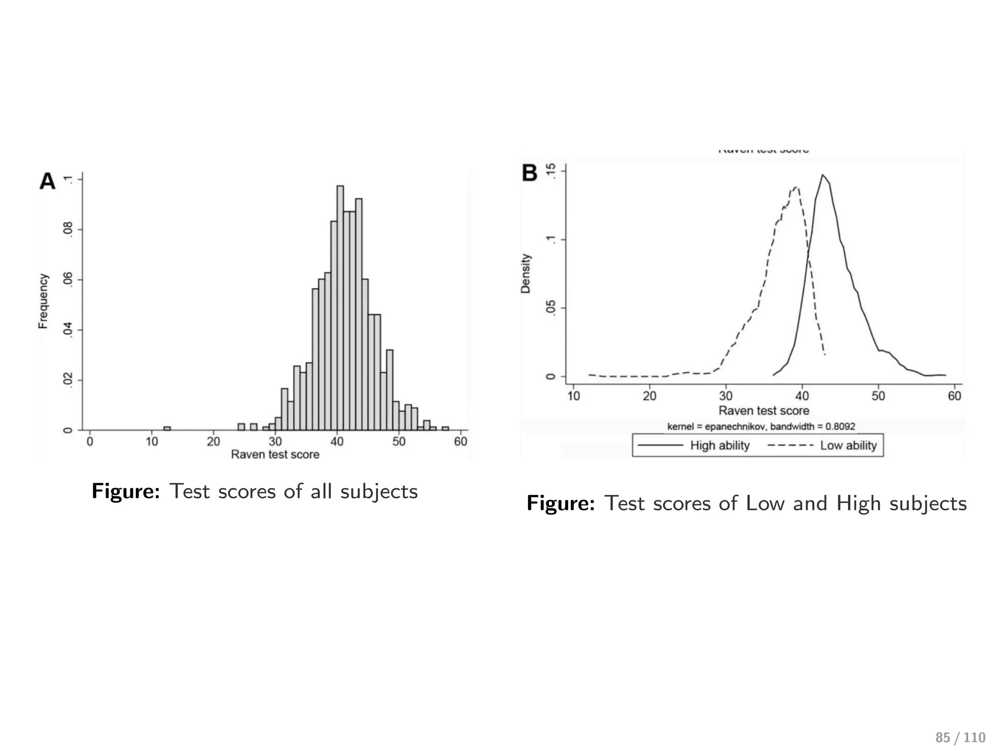
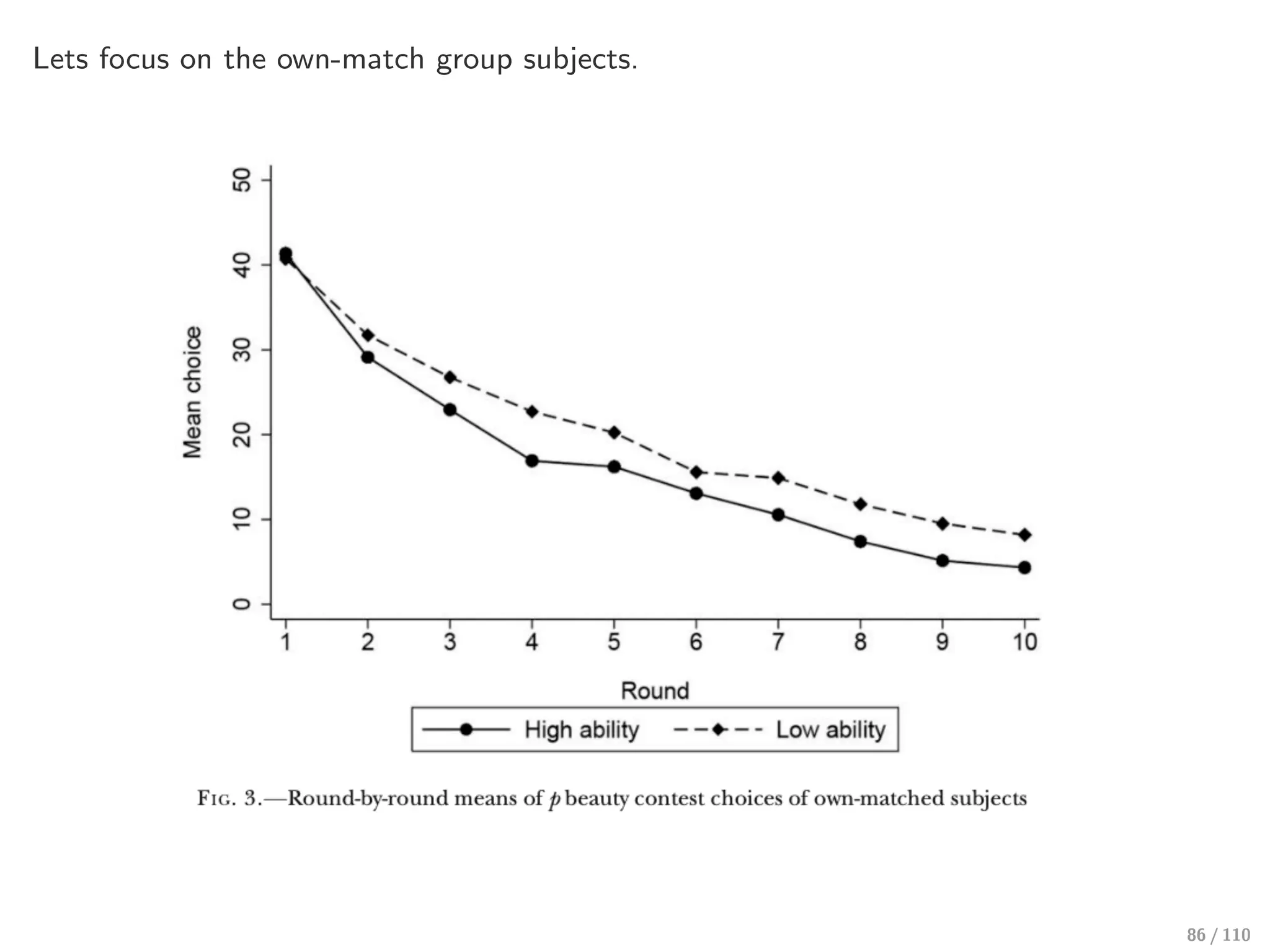
85.
Figure: Test scoresof all subjects
Figure: Test scores of Low and High subjects
85 / 110
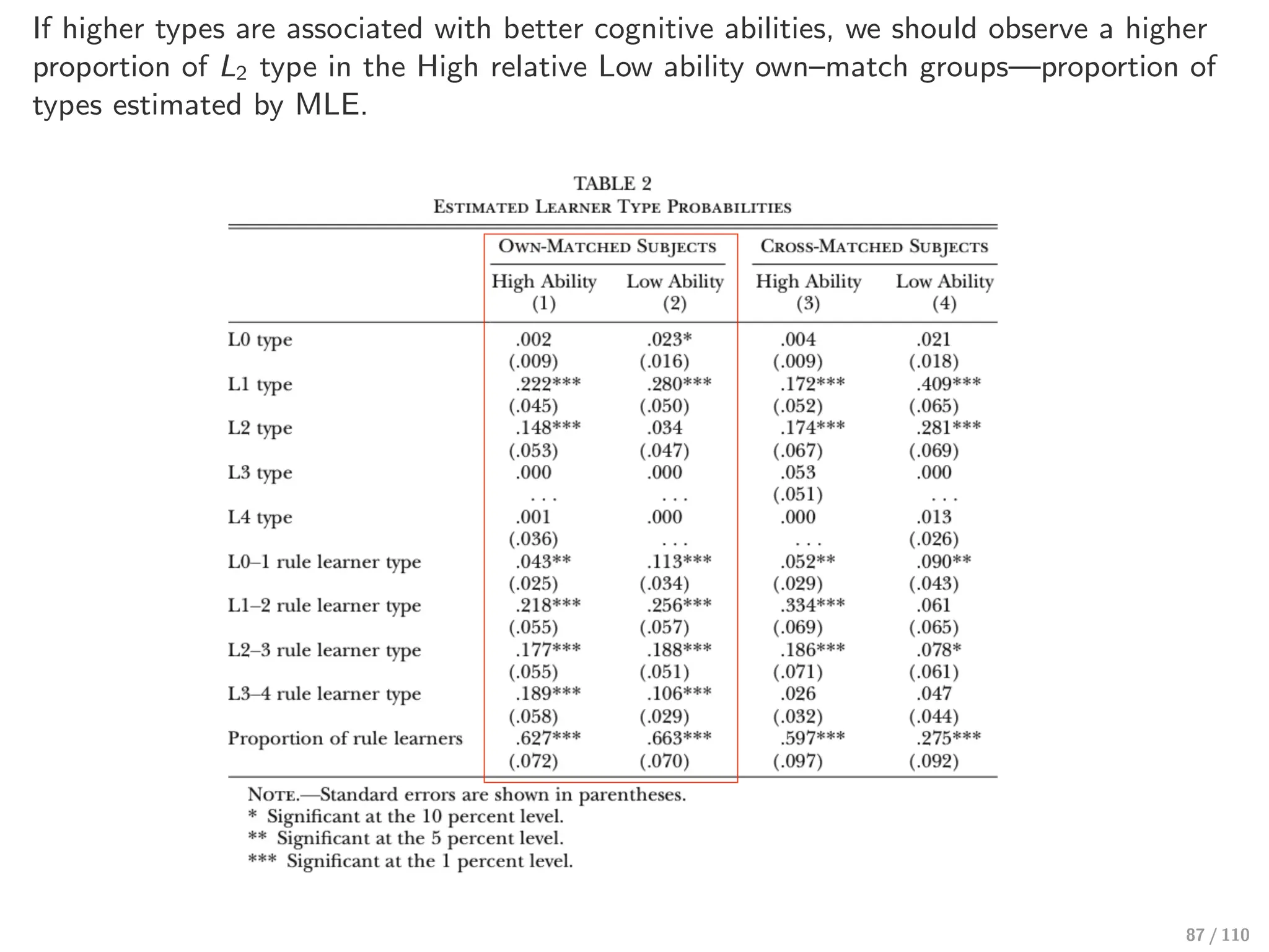
If higher typesare associated with better cognitive abilities, we should observe a higher
proportion of L2 type in the High relative Low ability own–match groups—proportion of
types estimated by MLE.
87 / 110
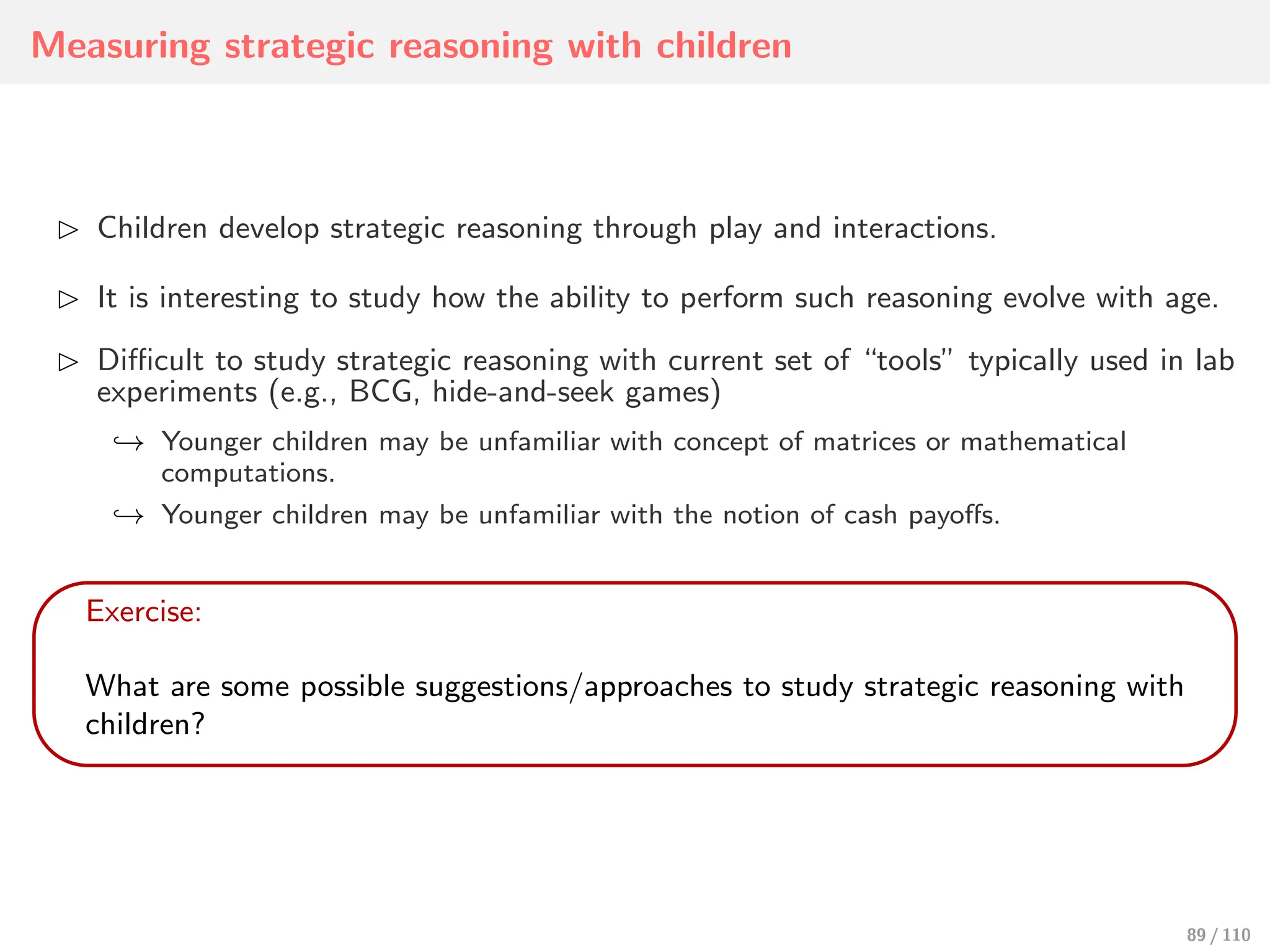
Measuring strategic reasoningwith children
⊲ Children develop strategic reasoning through play and interactions.
⊲ It is interesting to study how the ability to perform such reasoning evolve with age.
⊲ Difficult to study strategic reasoning with current set of “tools” typically used in lab
experiments (e.g., BCG, hide-and-seek games)
↩→ Younger children may be unfamiliar with concept of matrices or mathematical
computations.
↩→ Younger children may be unfamiliar with the notion of cash payoffs.
Exercise:
What are some possible suggestions/approaches to study strategic reasoning with
children?
89 / 110
90.
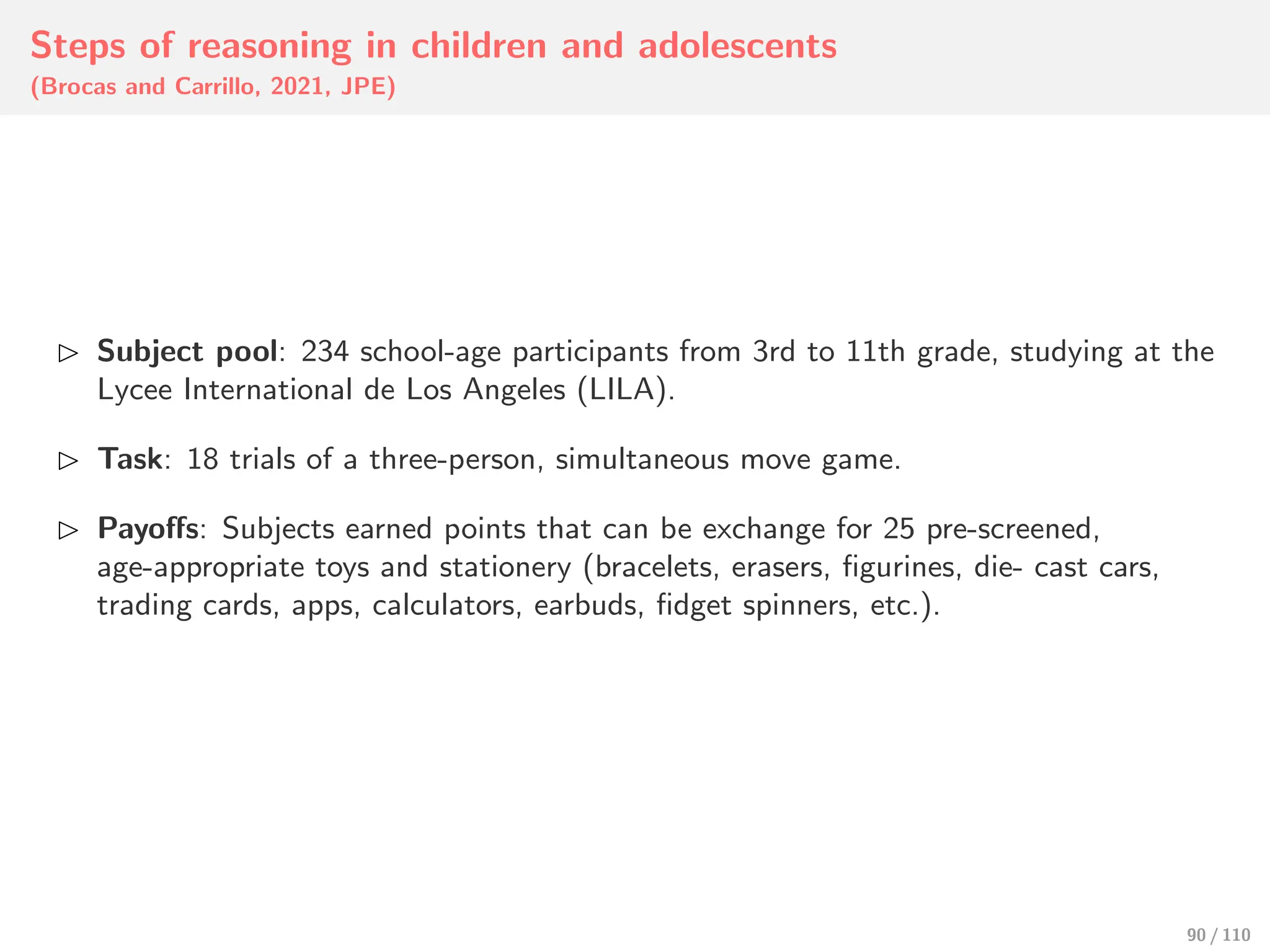
Steps of reasoningin children and adolescents
(Brocas and Carrillo, 2021, JPE)
⊲ Subject pool: 234 school-age participants from 3rd to 11th grade, studying at the
Lycee International de Los Angeles (LILA).
⊲ Task: 18 trials of a three-person, simultaneous move game.
⊲ Payoffs: Subjects earned points that can be exchange for 25 pre-screened,
age-appropriate toys and stationery (bracelets, erasers, figurines, die- cast cars,
trading cards, apps, calculators, earbuds, fidget spinners, etc.).
90 / 110
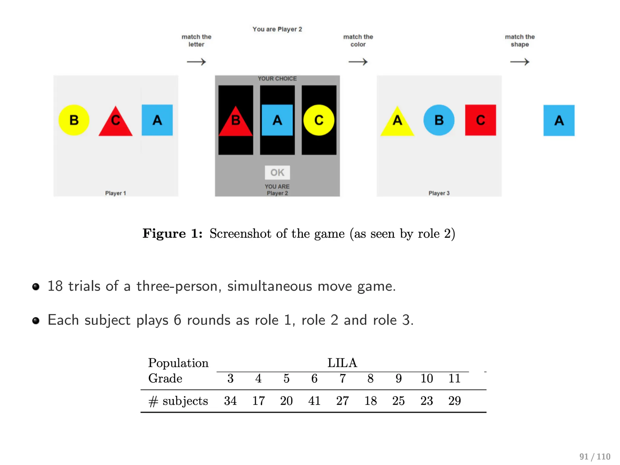
91.
18 trials ofa three-person, simultaneous move game.
Each subject plays 6 rounds as role 1, role 2 and role 3.
91 / 110
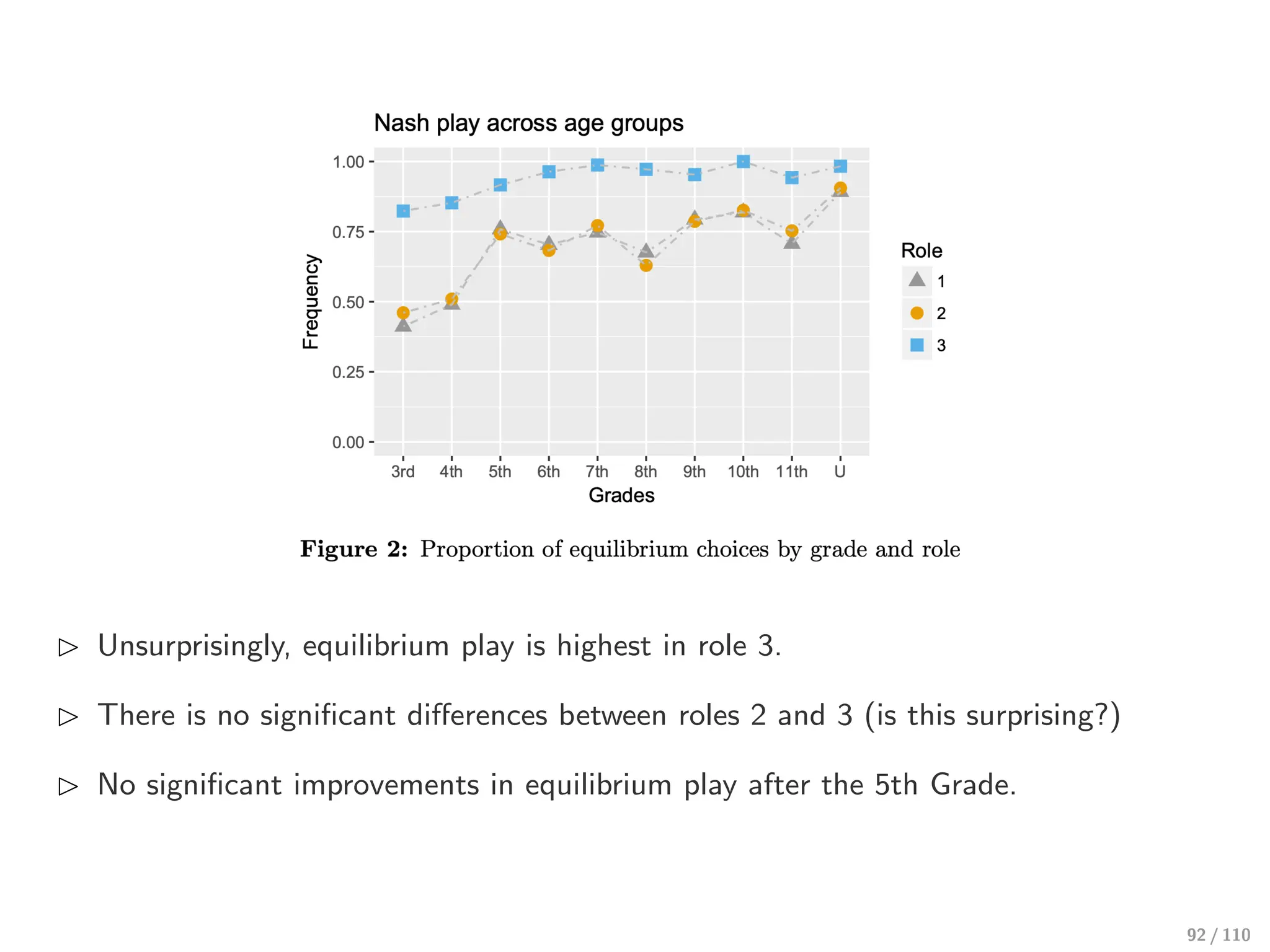
92.
⊲ Unsurprisingly, equilibriumplay is highest in role 3.
⊲ There is no significant differences between roles 2 and 3 (is this surprising?)
⊲ No significant improvements in equilibrium play after the 5th Grade.
92 / 110
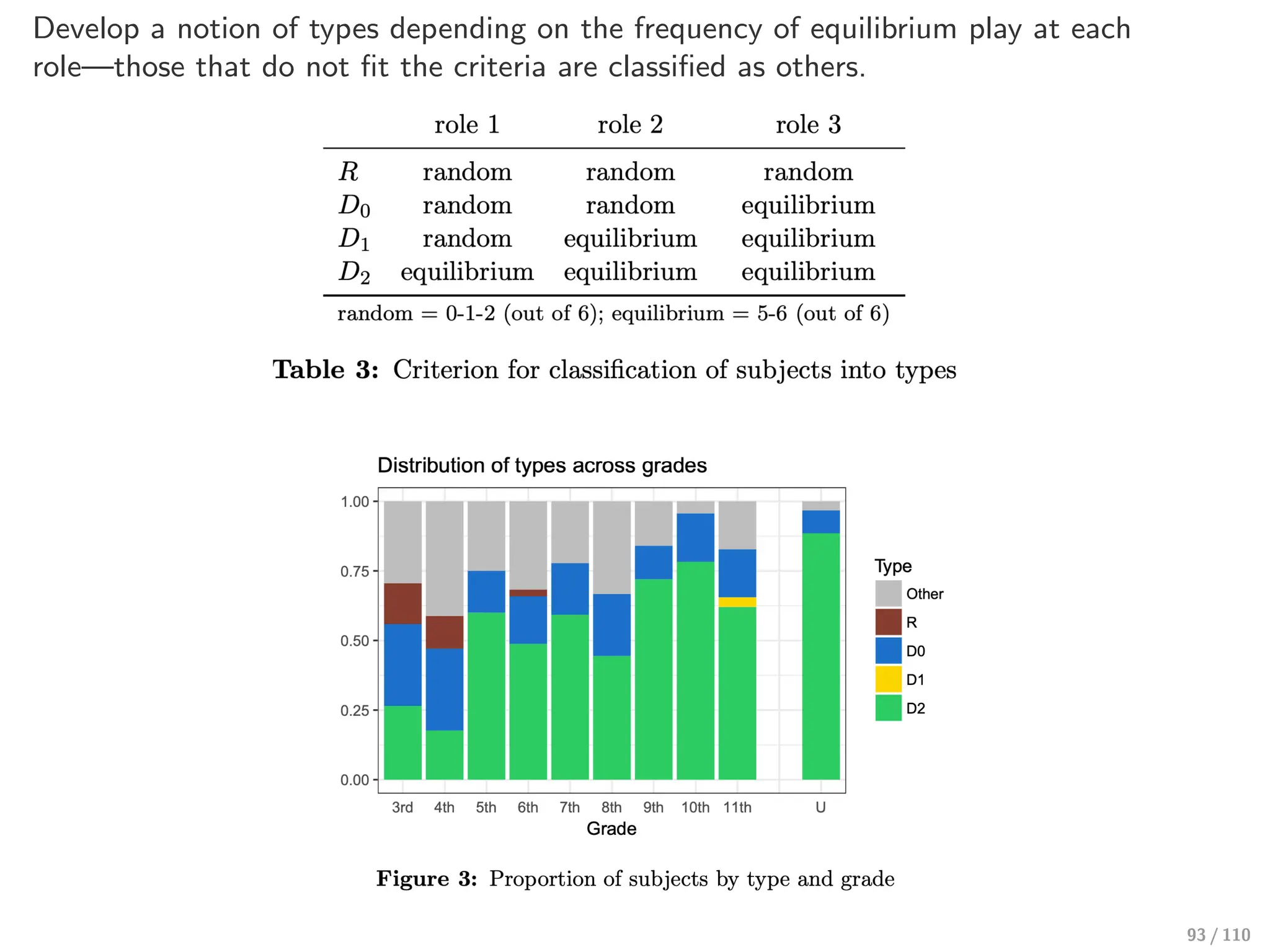
93.
Develop a notionof types depending on the frequency of equilibrium play at each
role—those that do not fit the criteria are classified as others.
93 / 110
94.
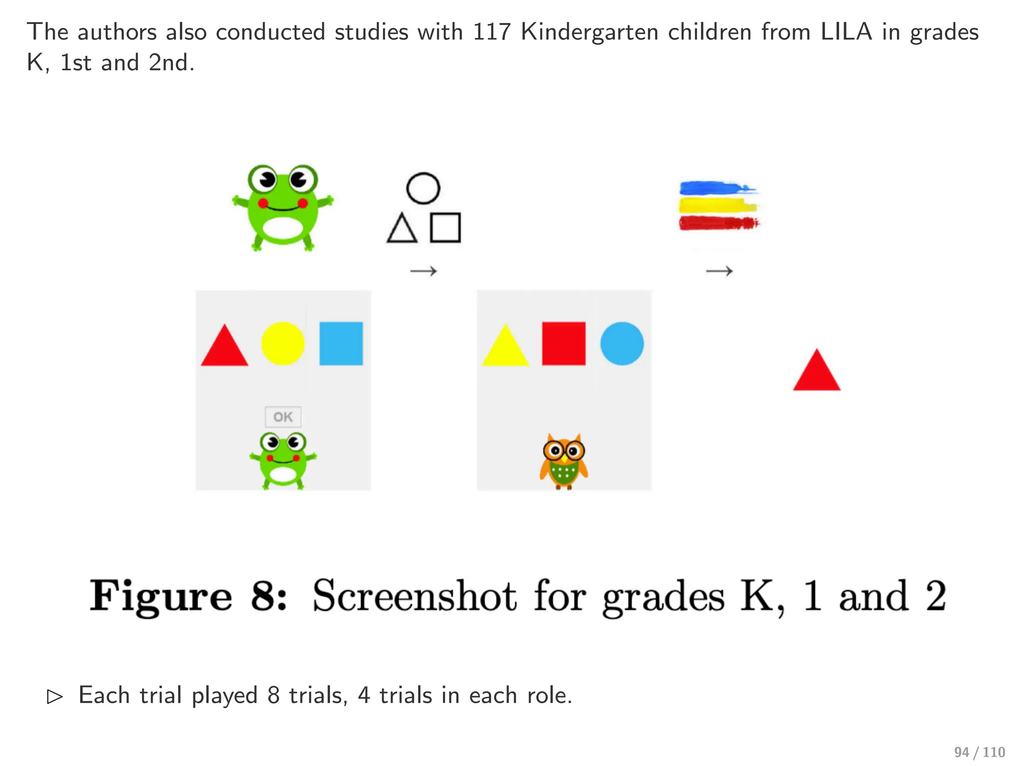
The authors alsoconducted studies with 117 Kindergarten children from LILA in grades
K, 1st and 2nd.
⊲ Each trial played 8 trials, 4 trials in each role.
94 / 110
95.
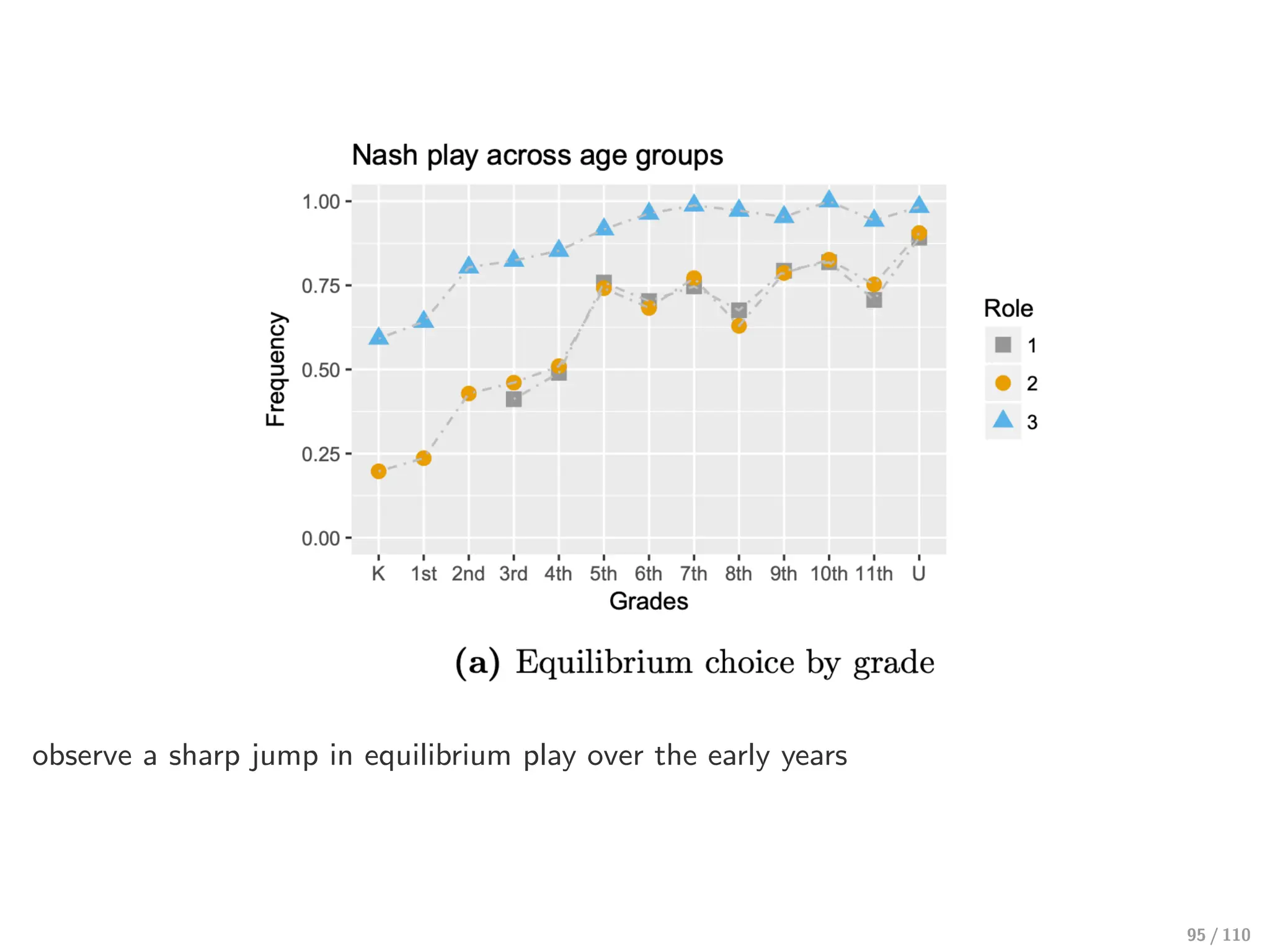
observe a sharpjump in equilibrium play over the early years
95 / 110
Cross-Game stability oftypes
⊲ The level-k model is used to ex-post explain the data through data-fitting.
⊲ The potential ex-ante use of the level-k model is to individual behaviour in
games—how would someone behave.
⊲ To do so, it can be beneficial to elicit a player’s Lk type and use it to predict his
behaviour across games.
⊲ The validity of the above requires cross game stability of types (i.e., player’s type to
be stable across games).
97 / 110
98.
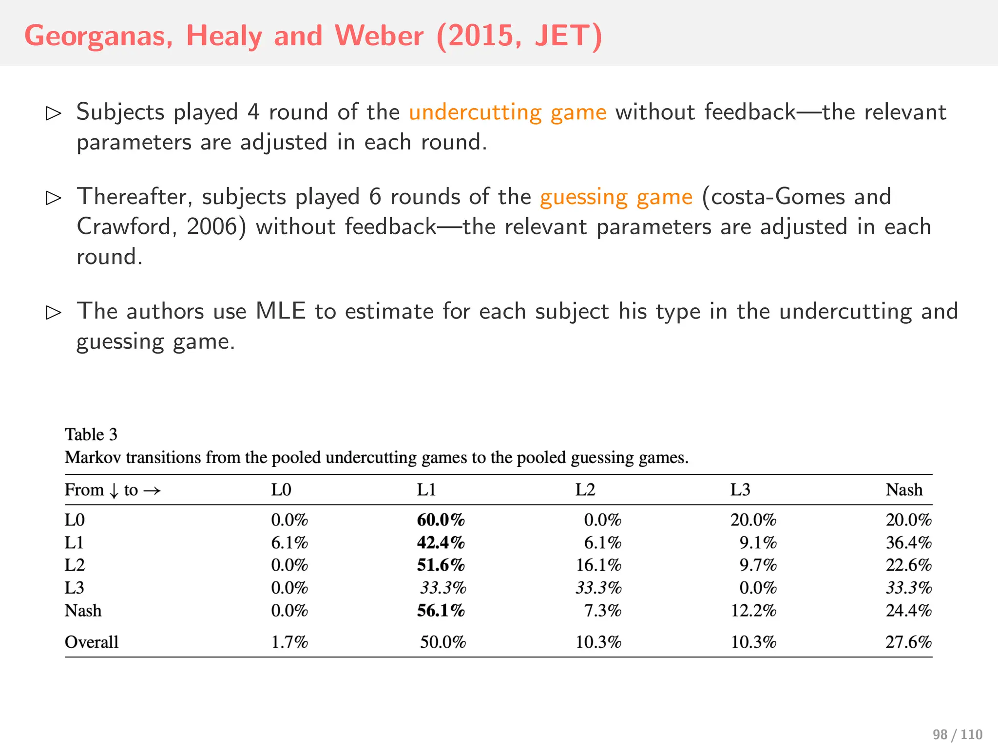
Georganas, Healy andWeber (2015, JET)
⊲ Subjects played 4 round of the undercutting game without feedback—the relevant
parameters are adjusted in each round.
⊲ Thereafter, subjects played 6 rounds of the guessing game (costa-Gomes and
Crawford, 2006) without feedback—the relevant parameters are adjusted in each
round.
⊲ The authors use MLE to estimate for each subject his type in the undercutting and
guessing game.
98 / 110
99.
Exercise:
In both games,Georganas et. al (2015) assumed that the L0 type will uniformly
randomise over all strategies.
Do you think that the instability of the types across games could be linked to the
saliency which we have previously discussed?
99 / 110
100.
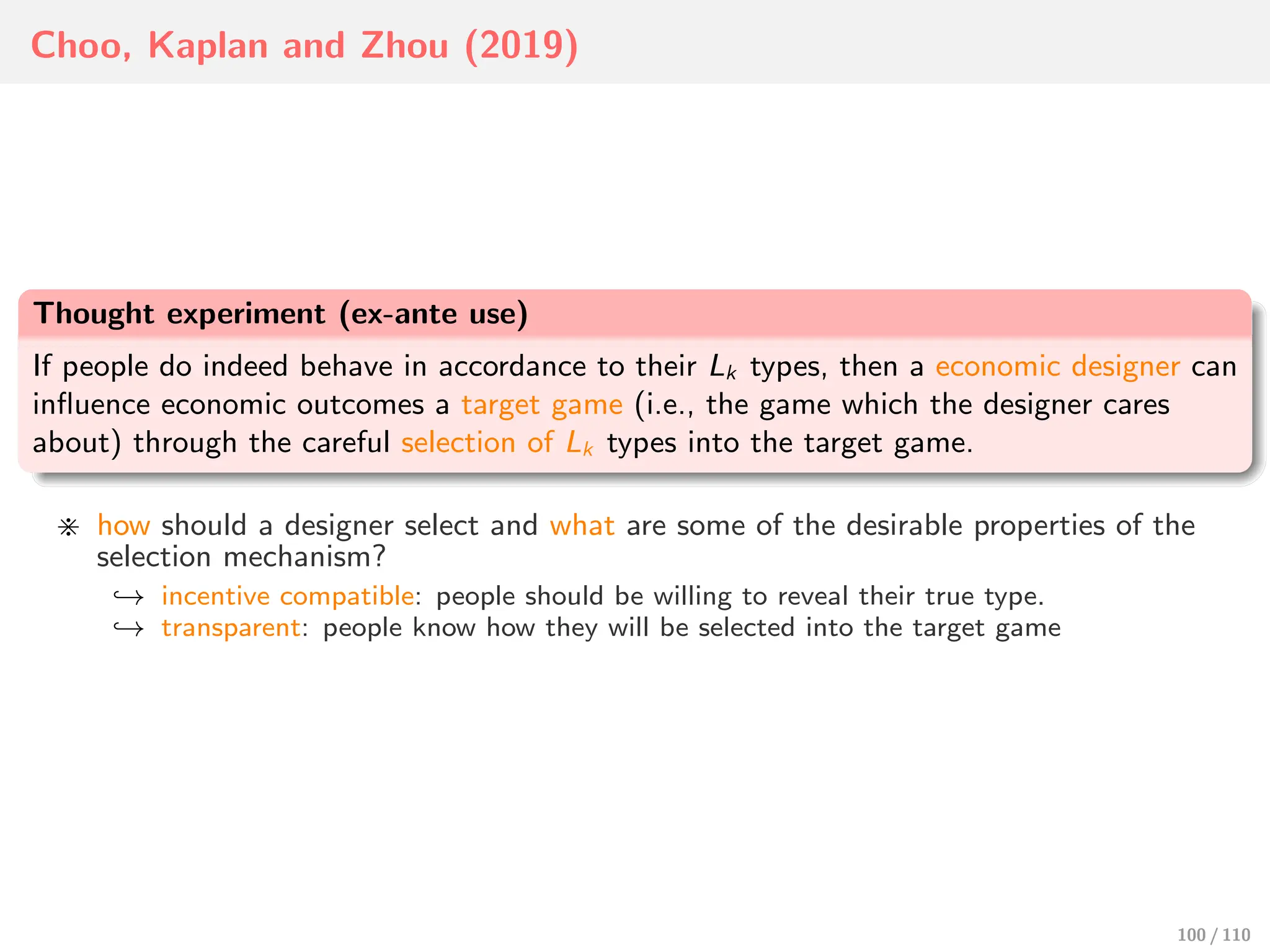
Choo, Kaplan andZhou (2019)
Thought experiment (ex-ante use)
If people do indeed behave in accordance to their Lk types, then a economic designer can
influence economic outcomes a target game (i.e., the game which the designer cares
about) through the careful selection of Lk types into the target game.
⋇ how should a designer select and what are some of the desirable properties of the
selection mechanism?
↩→ incentive compatible: people should be willing to reveal their true type.
↩→ transparent: people know how they will be selected into the target game
100 / 110
101.
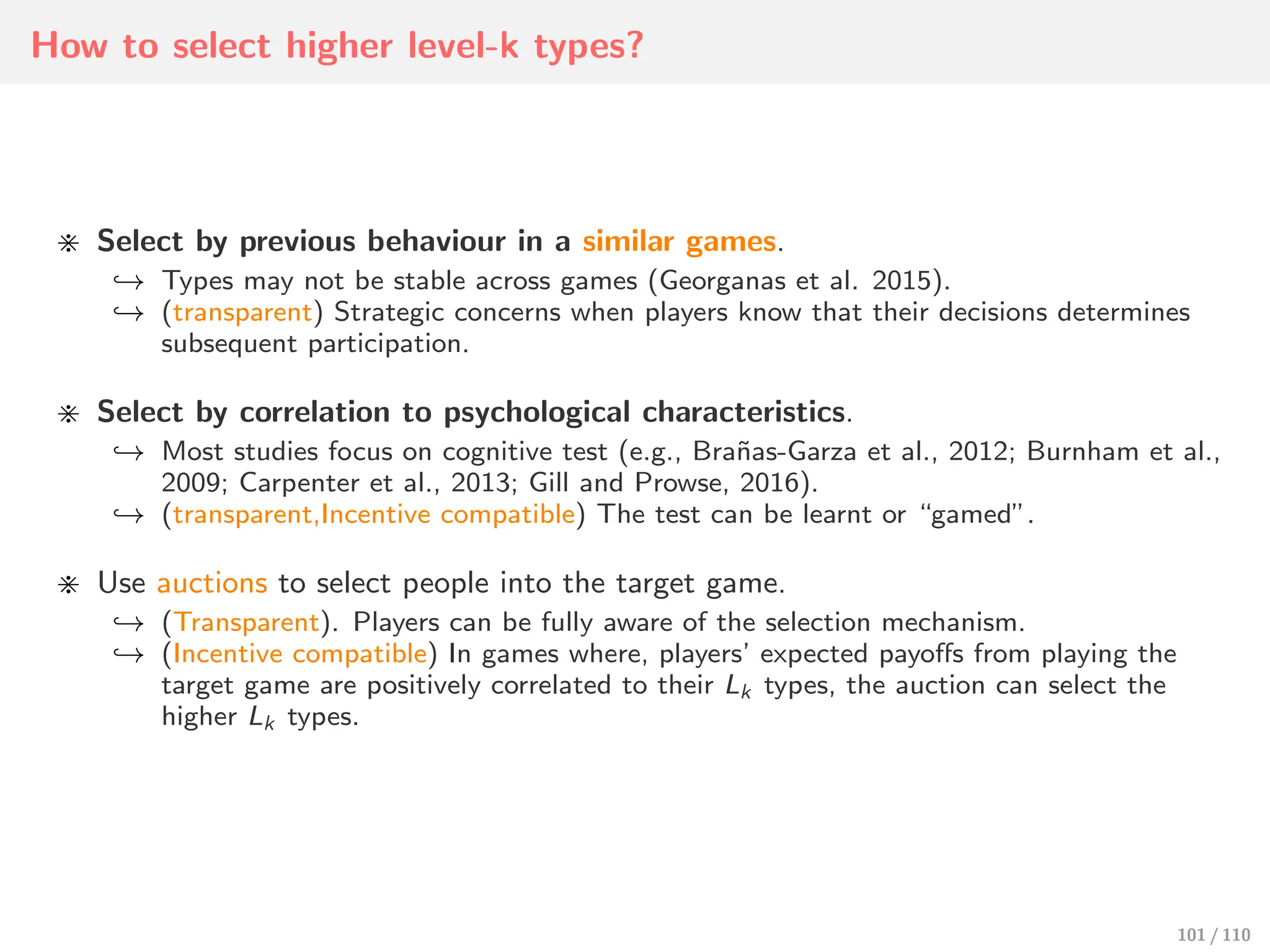
How to selecthigher level-k types?
⋇ Select by previous behaviour in a similar games.
↩→ Types may not be stable across games (Georganas et al. 2015).
↩→ (transparent) Strategic concerns when players know that their decisions determines
subsequent participation.
⋇ Select by correlation to psychological characteristics.
↩→ Most studies focus on cognitive test (e.g., Brañas-Garza et al., 2012; Burnham et al.,
2009; Carpenter et al., 2013; Gill and Prowse, 2016).
↩→ (transparent,Incentive compatible) The test can be learnt or “gamed”.
⋇ Use auctions to select people into the target game.
↩→ (Transparent). Players can be fully aware of the selection mechanism.
↩→ (Incentive compatible) In games where, players’ expected payoffs from playing the
target game are positively correlated to their Lk types, the auction can select the
higher Lk types.
101 / 110
102.
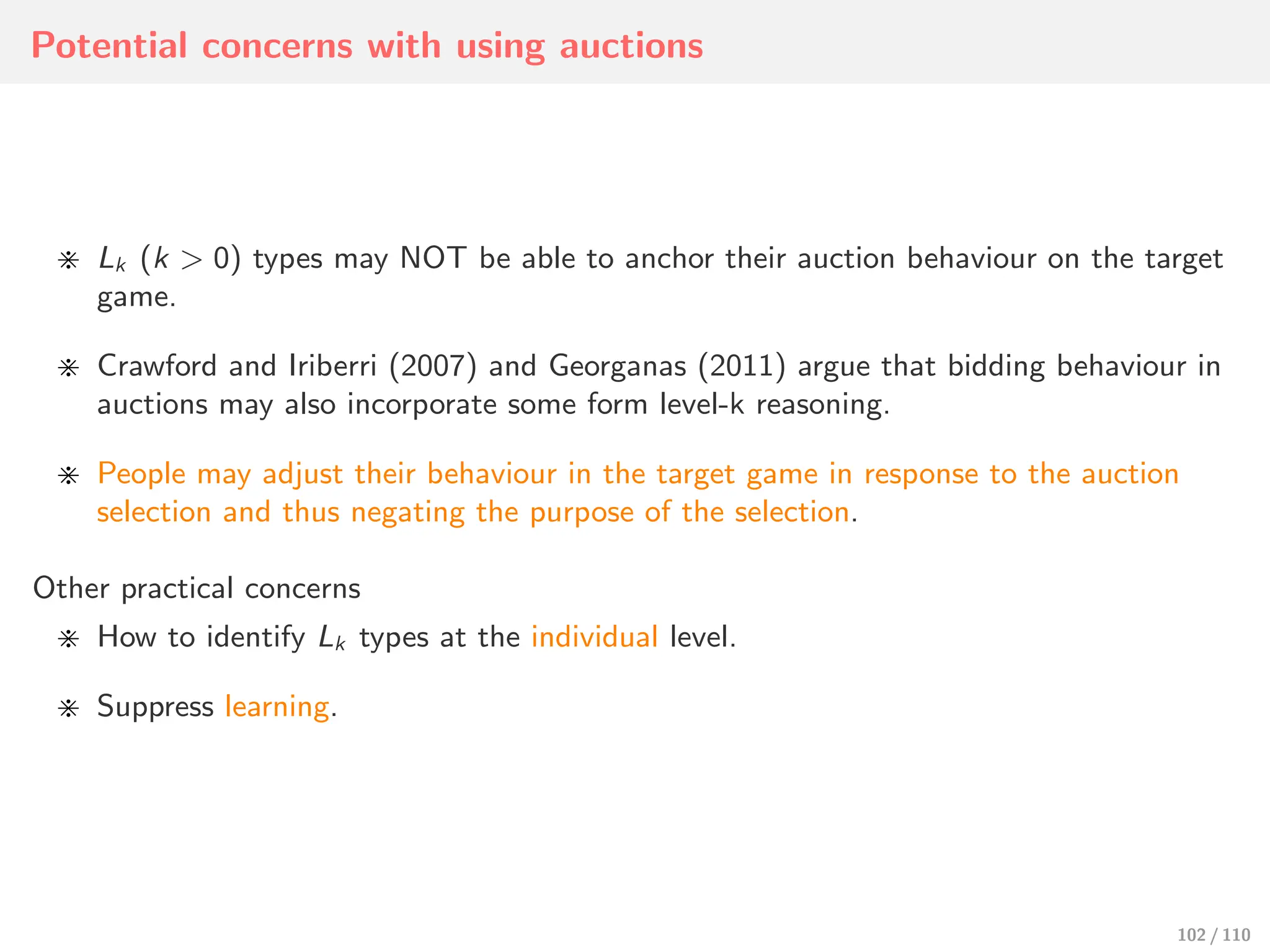
Potential concerns withusing auctions
⋇ Lk (k > 0) types may NOT be able to anchor their auction behaviour on the target
game.
⋇ Crawford and Iriberri (2007) and Georganas (2011) argue that bidding behaviour in
auctions may also incorporate some form level-k reasoning.
⋇ People may adjust their behaviour in the target game in response to the auction
selection and thus negating the purpose of the selection.
Other practical concerns
⋇ How to identify Lk types at the individual level.
⋇ Suppress learning.
102 / 110
103.
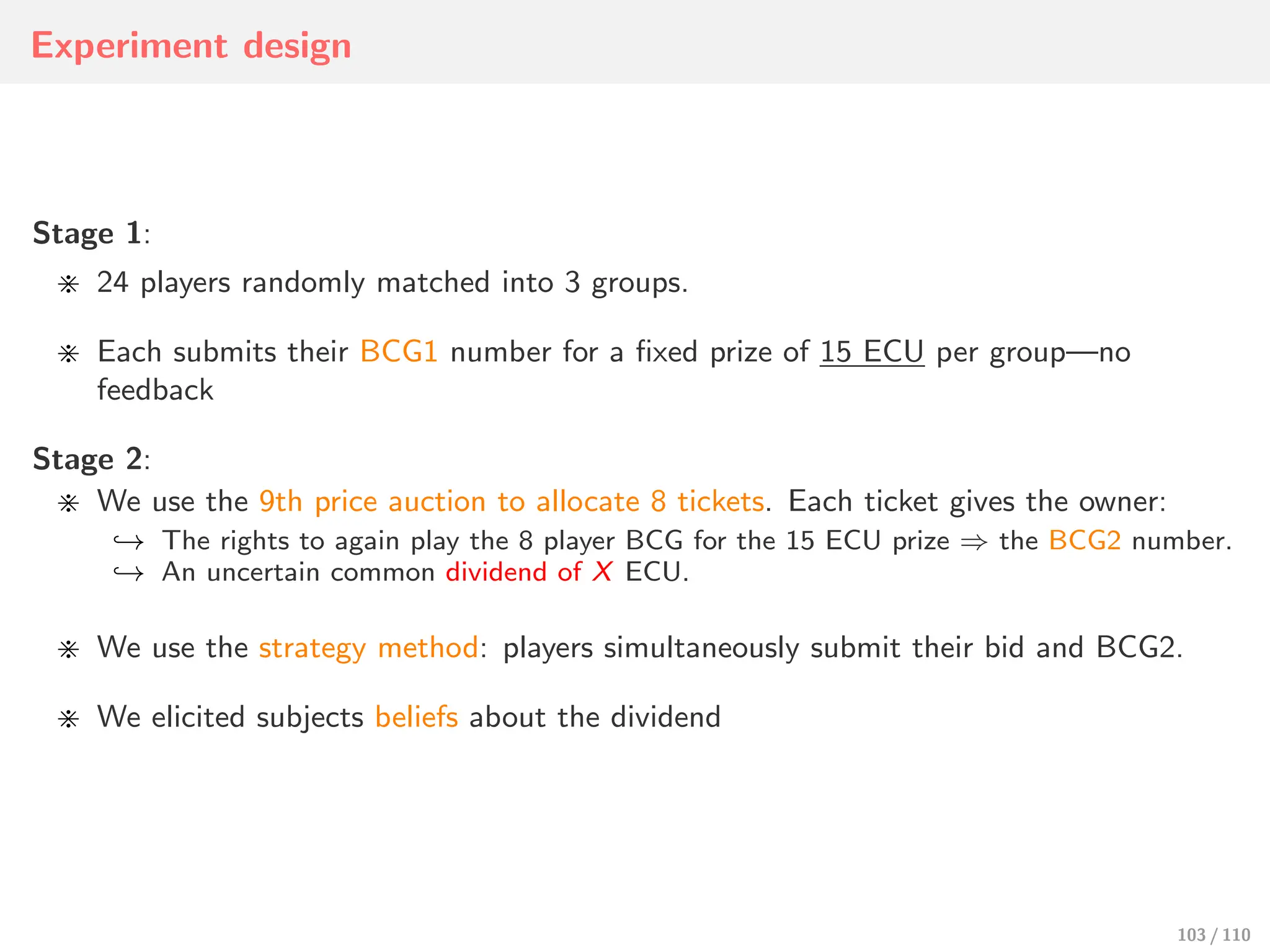
Experiment design
Stage 1:
⋇24 players randomly matched into 3 groups.
⋇ Each submits their BCG1 number for a fixed prize of 15 ECU per group—no
feedback
Stage 2:
⋇ We use the 9th price auction to allocate 8 tickets. Each ticket gives the owner:
↩→ The rights to again play the 8 player BCG for the 15 ECU prize ⇒ the BCG2 number.
↩→ An uncertain common dividend of X ECU.
⋇ We use the strategy method: players simultaneously submit their bid and BCG2.
⋇ We elicited subjects beliefs about the dividend
103 / 110
104.
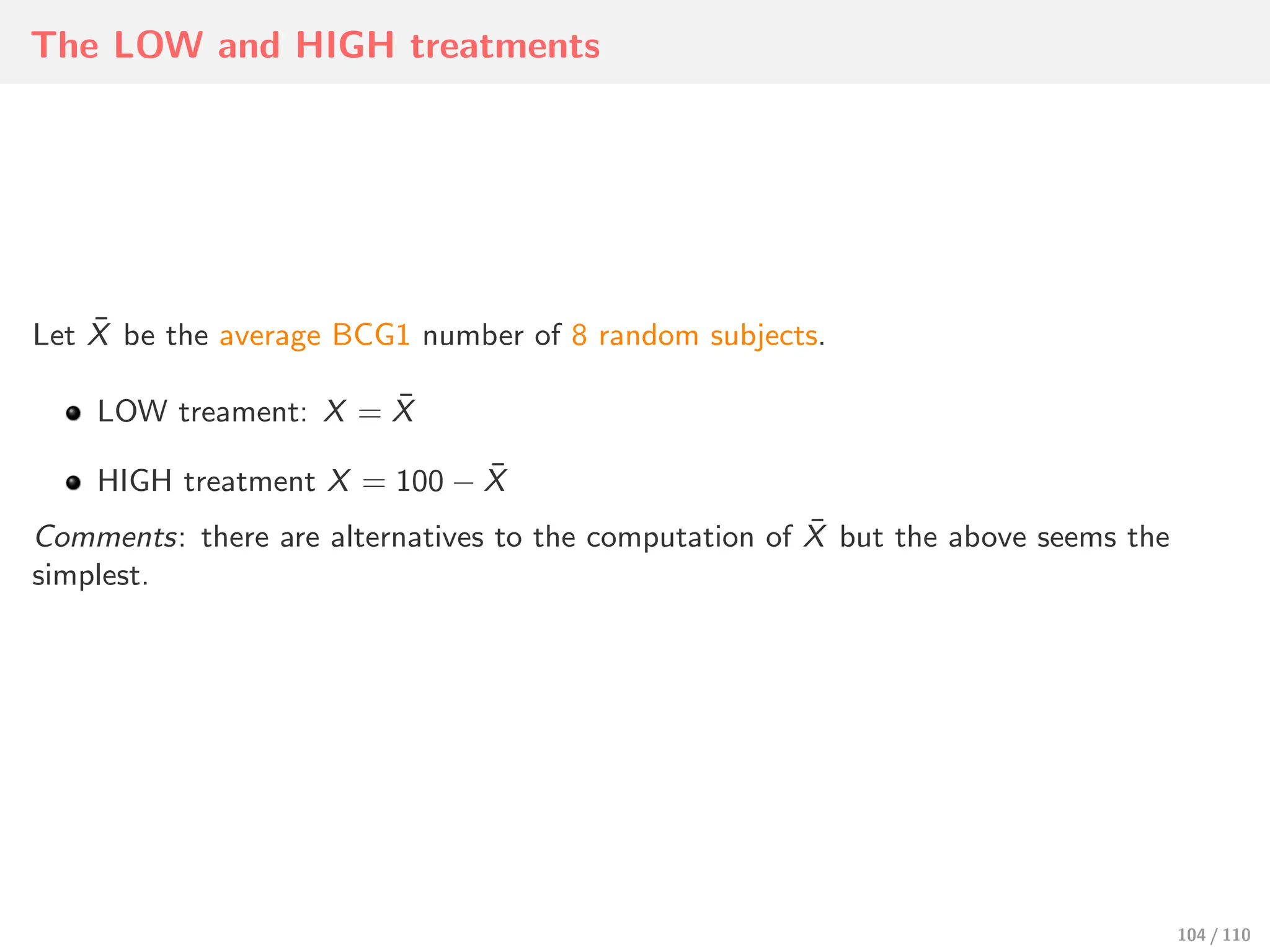
The LOW andHIGH treatments
Let X̄ be the average BCG1 number of 8 random subjects.
LOW treament: X = X̄
HIGH treatment X = 100 − X̄
Comments: there are alternatives to the computation of X̄ but the above seems the
simplest.
104 / 110
105.
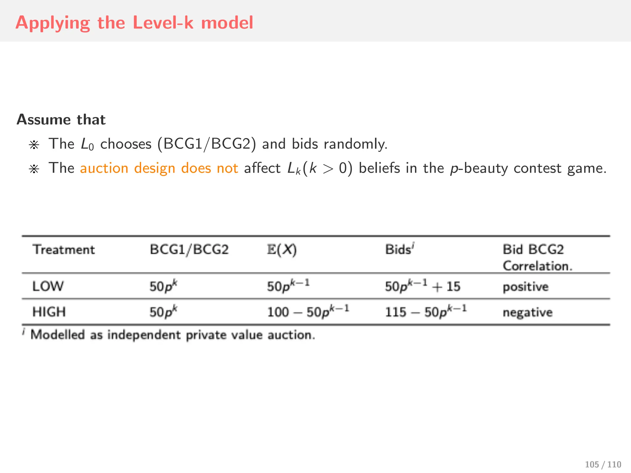
Applying the Level-kmodel
Assume that
⋇ The L0 chooses (BCG1/BCG2) and bids randomly.
⋇ The auction design does not affect Lk (k > 0) beliefs in the p-beauty contest game.
105 / 110
106.
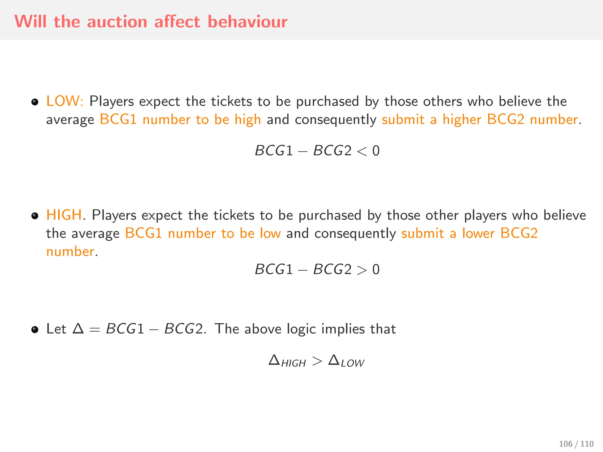
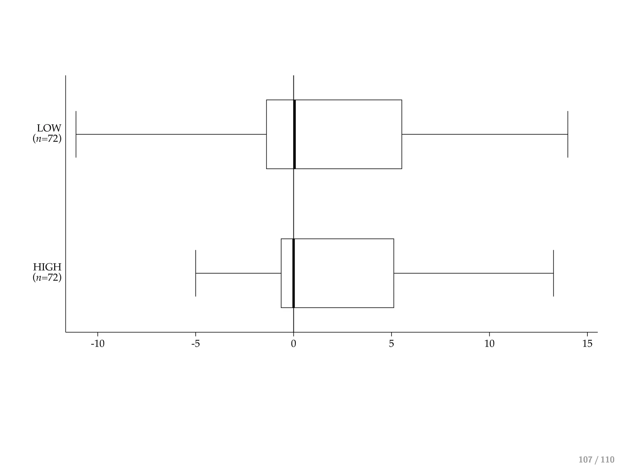
Will the auctionaffect behaviour
LOW: Players expect the tickets to be purchased by those others who believe the
average BCG1 number to be high and consequently submit a higher BCG2 number.
BCG1 − BCG2 < 0
HIGH. Players expect the tickets to be purchased by those other players who believe
the average BCG1 number to be low and consequently submit a lower BCG2
number.
BCG1 − BCG2 > 0
Let ∆ = BCG1 − BCG2. The above logic implies that
∆HIGH > ∆LOW
106 / 110
![Keynes Beauty contest
⊲ Consider a fictional newspaper contest, in which entrants are asked to choose the six
most attractive faces from a hundred photographs. Those who picked the most
popular faces are then eligible for a prize.
“It is not a case of choosing those [faces] that, to the best of one’s judgment,
are really the prettiest, nor even those that average opinion genuinely thinks the
prettiest.
We have reached the third degree where we devote our intelligences to anticipat-
ing what average opinion expects the average opinion to be.
And there are some, I believe, who practice the fourth, fifth and higher
degrees.”—(Keynes, General Theory of Employment, Interest and Money, 1936).
Exercise:
Can you think of economic situations that closely mirrors the beauty contest de-
scribed above?
20 / 110](https://image.slidesharecdn.com/slides3boundedrationalityandstrategicinteraction-250822000751-59107db0/75/Slides_3_Bounded_Rationality_and_Strategic_Interaction-pdf-20-2048.jpg)

![Strategic thinking
The canonical model of strategic thinking is the game-theoretic notion of Nash
equilibrium. Equilibrium is defined as a combination of strategies, one for each
player, such that each player’s strategy maximises his expected payoff, given the
others’ strategies.[...]
equilibrium is better justified in some applications than others. If players have
enough experience with analogous games, both theory and experimental results
suggest that learning has a strong tendency to converge to equilibrium.
If equilibrium is justified in such applications, it must be via strategic thinking
rather than learning.” — Crawford, Costa-Gomes and Iriberri (2013)
36 / 110](https://image.slidesharecdn.com/slides3boundedrationalityandstrategicinteraction-250822000751-59107db0/75/Slides_3_Bounded_Rationality_and_Strategic_Interaction-pdf-36-2048.jpg)
![Individual subject types without econometric
(Choo, Kaplan and Zhou, 2019)
⊲ Suppose that each subject plays the n = 8 BCG twice without feedback—let BCG1
and BCG2 be their choices in the first and second BCG, respectively.
⊲ By assumption, BCG1 and BCG2 will be random for the L0 type.
⊲ Whilst each Lk (k > 0) type might pick slightly different BCG1 and BCG2 numbers,
both numbers will be close to the same predicted Lk type number (i.e., 50pk
).
⊲ We construct a tolerance bandwidth for each Lk (k = 1, 2, ..., K̄) type—the
bandwidth around the predicted choice of each type.
↩→ L1 type bandwidth: [50p − e, 50p + e]
↩→ L2 type bandwidth: [50p2 − e, 50p2 + e]
↩→ ...
↩→ LK̄ type bandwidth: [0, 50pK̄ + e]
⊲ A subject is classified as type ˆ
Lk (k > 0) if both his BCG1 and BCG2 are within the
tolerance bandwidth of the Lk type—or otherwise a ˆ
L0 type.
Exercise:
How would you interpret the ˆ
L0 type?
47 / 110](https://image.slidesharecdn.com/slides3boundedrationalityandstrategicinteraction-250822000751-59107db0/75/Slides_3_Bounded_Rationality_and_Strategic_Interaction-pdf-47-2048.jpg)


![Game theory intro_and_questions_2009[1]](https://cdn.slidesharecdn.com/ss_thumbnails/gametheoryintroandquestions20091-140204051533-phpapp02-thumbnail.jpg?width=640&height=640&fit=bounds)