Downloaded 24 times


![General Form of the Far Field Solution
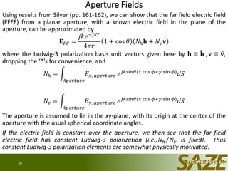
• In the far field of a finite radiating system in a homogeneous and isotropic
medium, we have the general solution
• The 𝐗 𝑙𝑚(𝜃, 𝜙) are the Vector Spherical Harmonics (VSHs) of degree 𝑙 and order
𝑚, where 𝑙 = 1, 2, 3, … and 𝑚 = −𝑙, −𝑙 + 1, … , −1, 0, +1, … , +𝑙. There are 2𝑙 +
1 orders 𝑚 for each degree 𝑙. Note that the VSHs 𝐗 𝑙𝑚 are transverse, i.e., 𝐫 ⋅
𝐗 𝑙𝑚 = 0. Mnemonic: degree𝑙 and 𝑚order.
• There is not a lot of literature on the VSHs, had to derive many results.
• (𝜃, 𝜙) are the ordinary angles from spherical coordinates (see Jackson)
• 𝚱 𝑙𝑚 and 𝚲𝑙𝑚 are arbitrary complex coefficients
• The 𝑃𝑙
𝑚
are the Associated Legendre Polynomials
Jackson, http://en.wikipedia.org/wiki/Associated_Legendre_polynomials
• The time-averaged Poynting vector is found from the electromagnetic phasors by
𝐒 =
1
2
Re 𝐄 × 𝐇∗ =
𝐄 2
2𝑍
𝐫 =
1
𝑟2
𝐕 2
2𝑍
𝐫, i.e., the power flows radially outward
5
ˆ)(coscot)(cosˆ)(coscsc
)!()1(4
)!)(12(
),(
ˆ
1
,]ˆ[
1
1
m
l
m
l
m
l
mj
lm
l
l
lm
lmlmlmlm
jkr
PmPjPme
mlll
mll
Zr
e
θΧ
ErHXrXE
FFR](https://image.slidesharecdn.com/10e522ed-4d24-4a0c-88ce-957574b8c880-160725222258/85/Fully-Polarimetric_Phased_Array_Far_Field_Modeling_2015SECONWorkshop_JHucks-5-320.jpg)
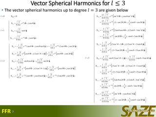
![Vector Spherical Harmonics (VSHs)
6
ˆ)(coscot)(cosˆ)(coscsc
)!()1(4
)!)(12(
),( 1
m
l
m
l
m
l
mj
lm PmPjPme
mlll
mll
θΧ
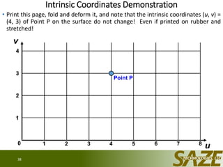
The following relationships between the vector spherical harmonics for m hold:
ml
m
lmlm
m
ml ,
11
, )1(,)1( ΧΧΧΧ
The vector spherical harmonics vanish for 0l or lm || :
lmorlforlm ||00),( Χ
The vector spherical harmonics lmX and their cross products with the unit radial vector lmXrˆ obey the sum
rule [Jackson]
4
12
),(),(),(ˆ),(
2222
l
XX
l
lm
lmlm
l
lm
lm
l
lm
lm XrX
and have the following orthogonality properties [Jackson]:
0sin)ˆ(,sin
2
0 0
2
0 0
dddd lmmlmmlllmml XrXXX
FFR](https://image.slidesharecdn.com/10e522ed-4d24-4a0c-88ce-957574b8c880-160725222258/85/Fully-Polarimetric_Phased_Array_Far_Field_Modeling_2015SECONWorkshop_JHucks-6-320.jpg)
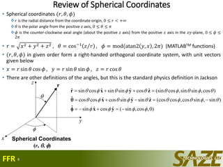
![Review of Spherical Harmonics (& Relation to VSHs)
9
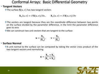
The spherical harmonics are given by [Jackson]
jmm
llm eP
ml
mll
Y )(cos
)!(4
)!)(12(
),(
The spherical harmonics for positive and negative m-values are related simply [Jackson]:
),()1(),(,
lm
m
ml YY
The spherical harmonics are normalized and orthogonal, in the following way [Jackson]:
mmlllmml YYdd
2
0 0
),(),(sin
The completeness relation is given by [Jackson]
)()cos(cos),(),(
0
l
l
lm
lmlm YY
The Xlm are the vector spherical harmonics, defined in Jackson as
)0(0
...),,3,2,1(),(
)1(
1
),(
l
lY
ll
lmlm LX
L denotes the angular momentum operator, familiar from quantum mechanics:
rL j
FFR
http://en.wikipedia.org/wiki/Spherical_harmonics
Kronecker delta
𝛿𝑖𝑗 = 1 if 𝑖 = 𝑗, 0 otherwise
(It is basically the identity matrix)](https://image.slidesharecdn.com/10e522ed-4d24-4a0c-88ce-957574b8c880-160725222258/85/Fully-Polarimetric_Phased_Array_Far_Field_Modeling_2015SECONWorkshop_JHucks-9-320.jpg)
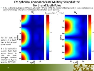
![Review of the Associated Legendre Polynomials
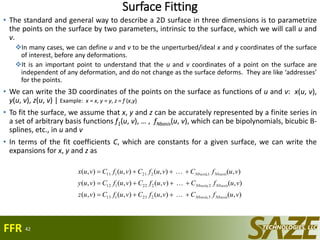
• Associated Legendre Polynomials of Degree 𝑙 and Order 𝑚
10
For ...,3,2,1,0l and llllm ,1,...,0,...,1, , the associated Legendre polynomials are given by the
following finite power series, derived from Rodrigues’ formula:
mkl
mlfloor
k
k
l
m
mm
l x
mklklk
klx
xP
2
]2/)([
0
2/2
)!2()!(!
)!22()1(
2
)1(
)1()(
The series above is valid for positive and negative integer values of m. The function floor(x) rounds the real
argument x down to the nearest integer less than or equal to x, and is a standard MATLABTM
function. The upper
sum limit prevents summation over terms that were differentiated away when the derivatives in Rodgrigues’ formula
were taken.
The associated Legendre polynomials vanish for lm || :
lmforxPm
l ||0)(
The following relationships between the associated Legendre polynomials for integer m hold:
)(
)!(
)!(
)1()(,)(
)!(
)!(
)1()( xP
ml
ml
xPxP
ml
ml
xP m
l
mm
l
m
l
mm
l
FFR
http://en.wikipedia.org/wiki/Legendre_polynomials
http://en.wikipedia.org/wiki/Associated_Legendre_polynomials](https://image.slidesharecdn.com/10e522ed-4d24-4a0c-88ce-957574b8c880-160725222258/85/Fully-Polarimetric_Phased_Array_Far_Field_Modeling_2015SECONWorkshop_JHucks-10-320.jpg)


![Spherical and Rectangular Bases
18
The spherical angle unit vectors are given by
yx
zyx
ˆcosˆsin)0,cos,sin(ˆ
ˆsinˆsincosˆcoscos)sin,sincos,cos(cosˆ
In the far field, the electric field E has only angular components, and their relationship to rectangular components is given by
zyx
zyxE
ˆ]0sin[ˆ]cossincos[ˆ]sincoscos[
ˆˆˆˆˆ),,(
EEEEEE
EEEEEEEE zyxzyx
This relationship may be summarized in matrix form (with the spherical components converted to Ludwig-3 components in the last step):
v
h
z
y
x
E
E
E
E
E
E
E
cossin
sincos
0sin
cossincos
sincoscos
0sin
cossincos
sincoscos
The spherical coordinate system becomes degenerate at the north and south poles ( = 0º and 180º, respectively). At the poles of the sphere, the
relationship above becomes (note that for a far field electric field, Ez = 0 at the poles, since the z component is longitudinal there)
18018000
cossin
sincos
,
cossin
sincos
E
E
E
E
E
E
E
E
y
x
y
x
The inverse relationships are given by
18018000
cossin
sincos
,
cossin
sincos
y
x
y
x
E
E
E
E
E
E
E
E
which shows that E and E are multivalued at the poles as varies from 0 to 180º, since physically the rectangular components must be well-
behaved everywhere.](https://image.slidesharecdn.com/10e522ed-4d24-4a0c-88ce-957574b8c880-160725222258/85/Fully-Polarimetric_Phased_Array_Far_Field_Modeling_2015SECONWorkshop_JHucks-18-320.jpg)
![Ludwig-3 Polarization Formulas
19
Ludwig-3 polarization components are given by defining the horizontal and vertical components to be given everywhere on the sphere by the same
expression as the rectangular components Ex and Ey are given in terms of E and E at the north pole:
E
E
E
E
v
h
cossin
sincos
At the north pole, Eh = Ex and Ev = Ey. The Ludwig-3 polarization components are well behaved at the north pole and the rest of the sphere except
the south pole, where they break down.
The spherical components may be given in terms of the Ludwig-3 components by using the inverse 2D rotation matrix to that above:
v
h
E
E
E
E
cossin
sincos
Since the Ludwig-3 components hE and vE are well-behaved and constant at the north pole, we see that the spherical components E and E will
have a sinusoidal dependence on there.
The Ludwig-3 unit polarization vectors can be shown to be given by
)ˆˆ(
ˆˆ1
ˆˆ
ˆ)ˆˆ(ˆ
cos1
)]ˆˆ(ˆ[ˆ
ˆ]sinsin[ˆ]sin)1(cos1[ˆ]sincos)1(cos[ˆ
)ˆˆ(
ˆˆ1
ˆˆ
ˆ)ˆˆ(ˆ
cos1
)]ˆˆ(ˆ[ˆ
ˆ]cossin[ˆ]sincos)1(cos[ˆ]cos)1(cos1[ˆ
2
2
zr
zr
yr
yzry
zryr
zyxv
zr
zr
xr
xzrx
zrxr
zyxh
zr
y
zr
x
At the north pole ( = 0°), the factor )1(cos vanishes and we see that xh ˆˆ and yv ˆˆ . At the south pole ( = 180°), the factor 2)1(cos ,
and we see that hˆ and vˆ are multiply valued vector functions of . Thus the Ludwig-3 polarization basis is good everywhere on the sphere except
the south pole. It should be noted that the Ludwig-3 basis is not a coordinate (holonomic) basis, but is a non-coordinate (anholonomic) basis.
](https://image.slidesharecdn.com/10e522ed-4d24-4a0c-88ce-957574b8c880-160725222258/85/Fully-Polarimetric_Phased_Array_Far_Field_Modeling_2015SECONWorkshop_JHucks-19-320.jpg)


,(
)exp(
),(
)exp(
),,( rrrkj
r
rkj
r
rkj
r EVVE
Thus we need to merely approximate rr in the far field where arr , . We have
ar
ar
ar
arar
ar
ar
ˆ
ˆ
ˆ
2
2
1
1
ˆ
21
ˆ
21
21)2(
2/12/1
2
2
2/1
2
2
2
2/122
rr
r
rr
r
rr
r
a
r
rr
r
a
r
rrarrrr
so that
),,()exp(
),,()ˆexp(
),,()](exp[),,(
rj
rkj
rrrkjr
Eak
Ear
EE
which completes the proof. The ‘Array Factor’ )exp( ak j is an angular and frequency dependent phase term that multiplies the pattern of an element
or subarray at the origin to account for the translation of the radiating system’s phase center by a vector distance a .
FFR](https://image.slidesharecdn.com/10e522ed-4d24-4a0c-88ce-957574b8c880-160725222258/85/Fully-Polarimetric_Phased_Array_Far_Field_Modeling_2015SECONWorkshop_JHucks-26-320.jpg)


![MATLABTM Function to Compute Active Rotation Matrix% % % J. Hucks, SAZE Technologies, LLC
%
% R=Rfromaxisangle(axis,alphadeg)
%
% This function computes the 3x3 real active rotation matrix given the axis
% of rotation and the rotation angle.
%
% axis is a 3x1 unit column vector with the x, y and z components of the
% axis of rotation. If it is not a unit vector, it is normalized, so it
% does not have to be a unit vector, but must be parallel to the axis of
% rotation.
%
% alphadeg is the real angle of the rotation in degrees, using the RH rule
% convention, where the right thumb points in the direction of the axis of
% rotation, and the fingers curl in the direction of the rotation (if the
% rotation angle is positive).
function R=Rfromaxisangle(axis,alphadeg)
% 1 degree in radians
deg=pi/180;
% Convert alphadeg to radians
alpha=alphadeg*deg;
% Make sure axis is a unit vector
e=axis/norm(axis);
% Separate out the components of e for computation to follow
e1=e(1); e2=e(2); e3=e(3);
% Define needed trig functions of alpha
ca=cos(alpha); sa=sin(alpha); omca=1-ca;
% Compute the 3x3 active rotation matrix R
R=[ ca+e1^2*omca e1*e2*omca-e3*sa e1*e3*omca+e2*sa;
e1*e2*omca+e3*sa ca+e2^2*omca e2*e3*omca-e1*sa;
e1*e3*omca-e2*sa e2*e3*omca+e1*sa ca+e3^2*omca ];
31
• Implements the formula from the previous slide for
computing an active rotation matrix by computing its
components
• Inputs are a unit vector giving the axis of rotation and an
angle in degrees giving the angle of rotation, with the
RH rule applying
• This function computes 1 active rotation matrix from a
single axis and angle of rotation
• To get a passive rotation matrix for the same axis and
angle, simply input the opposite axis or angle. Putting in
the opposite axis and opposite angle will give you the
same active rotation matrix.
• Can also use the alternative result for an active rotation
matrix
𝐑 = exp 𝛼
0 −𝑒3 𝑒2
𝑒3 0 −𝑒1
−𝑒2 𝑒1 0
• In the above, the MATLABTM matrix exponential function
expm function should be used, and not the element-by-
element exponential function exp; however, this
formulation is computationally more intensive and will
be less accurate due to slower convergence.
• Can use MATLABTM function logm, inverse of expm, to
solve for axis and angle of rotation of a rotation matrix.
• Rfromaxisangle is free to use and distribute with
attribution
FFR
• Note that if we form a 3 × 𝑁 matrix with 3D vectors in
its 𝑁 columns and multiply on the left by a 3 × 3
rotation matrix 𝐑, the resultant 3 × 𝑁 matrix is the
previous matrix with each column multiplied by 𝐑
This can be useful in vectorizing code when we
are rotating many vectors simultaneously, all with
the same rotation matrix](https://image.slidesharecdn.com/10e522ed-4d24-4a0c-88ce-957574b8c880-160725222258/85/Fully-Polarimetric_Phased_Array_Far_Field_Modeling_2015SECONWorkshop_JHucks-31-320.jpg)


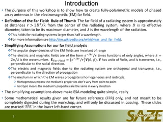
This document provides an introduction to modeling fully-polarimetric phased array antennas in the electromagnetic far field. It defines the far field region and outlines simplifying assumptions used in the analysis. Maxwell's equations and their time-harmonic form are reviewed. The general form of the far field solution is presented using vector spherical harmonics. Examples of vector spherical harmonics for degrees l=0 to 3 are also provided.


