Download to read offline

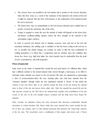
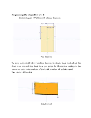
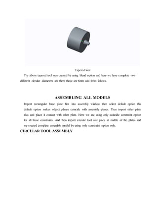
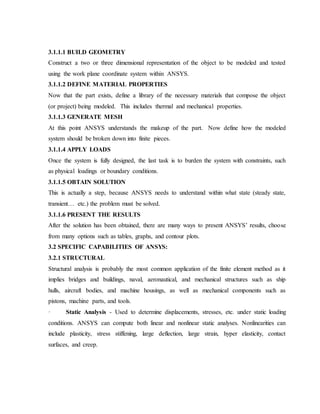
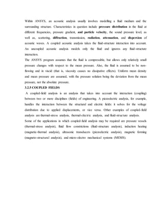
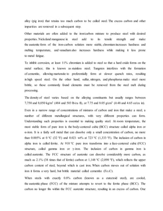
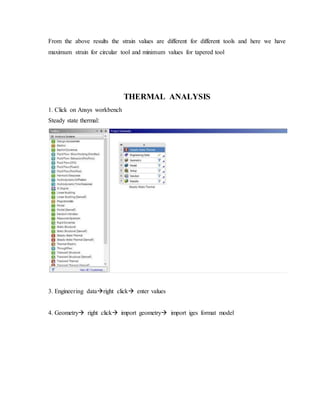
![Friction stir welding schematic diagram
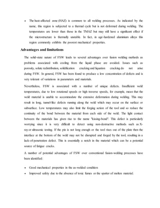
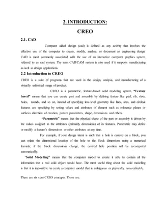
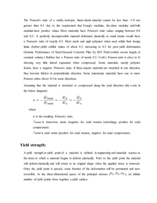
Micro structural features
The solid-state nature of the FSW process, combined with its unusual tool and asymmetric
nature, results in a highly characteristic microstructure. The microstructure can be broken up into
the following zones:
The stir zone (also nugget, dynamically recrystallised zone) is a region of heavily
deformed material that roughly corresponds to the location of the pin during welding.
The grains within the stir zone are roughly equiaxed and often an order of magnitude
smaller than the grains in the parent material. A unique feature of the stir zone is the
common occurrence of several concentric rings which has been referred to as an "onion-
ring" structure. The precise origin of these rings has not been firmly established, although
variations in particle number density, grain size and texture have all been suggested.
The flow arm zone is on the upper surface of the weld and consists of material that is
dragged by the shoulder from the retreating side of the weld, around the rear of the tool,
and deposited on the advancing side.
The thermo-mechanically affected zone (TMAZ) occurs on either side of the stir zone. In
this region the strain and temperature are lower and the effect of welding on the
microstructure is correspondingly smaller. Unlike the stir zone the microstructure is
recognizably that of the parent material, albeit significantly deformed and rotated.
Although the term TMAZ technically refers to the entire deformed region it is often used
to describe any region not already covered by the terms stir zone and flow arm.[citation needed]](https://image.slidesharecdn.com/frictionstirwelding-220121065424/85/Friction-stir-welding-3-320.jpg)
![landing platforms at Marine Aluminium Aanensen. Marine Aluminium Aanensen subsequently
merged with Hydro Aluminium Maritime to become Hydro Marine Aluminium. Some of these
freezer panels are now produced by Riftec and Bayards. In 1997 two-dimensional friction stir
welds in the hydro dynamically flared bow section of the hull of the ocean viewer vessel The
Boss were produced at Research Foundation Institute with the first portable FSW machine.
The Super Liner Ogasawara at Mitsui Engineering and Shipbuilding is the largest friction stir
welded ship so far. The Sea Fighter of Nichols Bros and the Freedom Littoral Combat
Ships contain prefabricated panels by the FSW fabricators Advanced Technology and Friction
Stir Link, Inc. respectively. The Houbei class missile boat has friction stir welded rocket launch
containers of China Friction Stir Centre. HMNZSRotoiti in New Zealand has FSW panels made
by Donovans in a converted milling machine. Various companies apply FSW to armor
plating for amphibious assault ships
Aerospace
United Launch Alliance applies FSW to the Delta II, Delta IV, and Atlas V expendable launch
vehicles, and the first of these with a friction stir welded Interstage module was launched in
1999. The process is also used for the Space Shuttle external tank, for Ares I and for the
Orion test article at NASA as well as Falcon 1 and Falcon 9 rockets at SpaceX. The toe nails for
ramp of Boeing C-17 Globemaster III cargo aircraft by Advanced Joining Technologies[39] and
the cargo barrier beams for the Boeing 747 Large Cargo Freighter[39] were the first commercially
produced aircraft parts. FAA approved wings and fuselage panels of the Eclipse 500 aircraft
were made at Eclipse Aviation, and this company delivered 259 friction stir welded business jets,
before they were forced into Chapter 7 liquidation. Floor panels for Airbus A400M military
aircraft are now made by Pfalz Flugzeugwerke and Embraer used FSW for the Legacy 450 and
500 Jets Friction stir welding also is employed for fuselage panels on the Airbus
A380. BRÖTJE-Automation GmbH uses friction stir welding – through the DeltaN FS system –
for gantry production machines developed for the aerospace sector as well as other industrial
applications
Automotive
Aluminium engine cradles and suspension struts for stretched Lincoln Town Car were the first
automotive parts that were friction stir at Tower, who use the process also for the engine tunnel](https://image.slidesharecdn.com/frictionstirwelding-220121065424/85/Friction-stir-welding-11-320.jpg)
![of the Ford GT. A spin-off of this company is called Friction Stir Link, Inc. and successfully
exploits the FSW process, e.g. for the flatbed trailer "Revolution" of Fontaine Trailers.[43] In
Japan FSW is applied to suspension struts at Showa Denko and for joining of aluminium sheets
to galvanized steel brackets for the boot (trunk) lid of the Mazda MX-5. Friction stir spot
welding is successfully used for the bonnet (hood) and rear doors of the Mazda RX-8 and the
boot lid of the Toyota Prius. Wheels are friction stir welded at Simmons Wheels, UT Alloy
Works and Fundo. Rear seats for the Volvo V70 are friction stir welded at Sapa, HVAC pistons
at Halla Climate Control and exhaust gas recirculation coolers at Pierburg. Tailor welded
blanks are friction stir welded for the Audi R8 at Riftec. The B-column of the Audi R8 Spider is
friction stir welded from two extrusions at Hammerer Aluminium Industries in Austria.
Railways
Since 1997 roof panels were made from aluminium extrusions at Hydro Marine
Aluminium with a bespoke 25m long FSW machine, e.g. for DSB class SA-SD trains of Alstom
LHB Curved side and roof panels for the Victoria line trains of London Underground, side
panels for Bombardier's Electrostar trains at Sapa Group and side panels for Alstom's British
Rail Class 390 Pendolino trains are made at Sapa Group Japanese commuter and express A-
trains, and British Rail Class 395 trains are friction stir welded
byHitachi, while Kawasaki applies friction stir spot welding to roof panels and Sumitomo Light
Metal produces Shinkansen floor panels. Innovative FSW floor panels are made by Hammerer
Aluminium Industries in Austria for the Stadler KISS double decker rail cars, to obtain an
internal height of 2 m on both floors and for the new car bodies of the Wuppertal Suspension
Railway. Heat sinks for cooling high-power electronics of locomotives are made at Sykatek,
EBG, Austerlitz Electronics, Euro Composite, Sapa and Rapid Technic, and are the most
common application of FSW due to the excellent heat transfer
Fabrication
Façade panels and athode sheets are friction stir welded at AMAG and Hammerer Aluminium
Industries including friction stir lap welds of copper to aluminium. Bizerba meat slicers,
Ökolüfter HVAC units and Siemens X-ray vacuum vessels are friction stir welded at Riftec.
Vacuum valves and vessels are made by FSW at Japanese and Swiss companies. FSW is also
used for the encapsulation of nuclear waste at SKB in 50-mm-thick copper canisters. Pressure](https://image.slidesharecdn.com/frictionstirwelding-220121065424/85/Friction-stir-welding-12-320.jpg)
![way for carbon to leave the austenite is for it to precipitate out of solution as cementite,
leaving behind a surrounding phase of BCC iron called ferrite that is able to hold the carbon
in solution. The two, ferrite and cementite, precipitate simultaneously producing a layered
structure called pearlite, named for its resemblance to mother of pearl. In a hypereutectoid
composition (greater than 0.8% carbon), the carbon will first precipitate out as large
inclusions of cementite at the austenite grain boundaries and then when the composition left
behind is eutectoid, the pearlite structure forms. For steels that have less than 0.8% carbon
(hypoeutectoid), ferrite will first form until the remaining composition is 0.8% at which point
the pearlite structure will form. No large inclusions of cementite will form at the
boundaries.[8] The above assumes that the cooling process is very slow, allowing enough time
for the carbon to migrate.
As the rate of cooling is increased the carbon will have less time to migrate to form carbide at
the grain boundaries but will have increasingly large amounts of pearlite of a finer and finer
structure within the grains; hence the carbide is more widely dispersed and acts to prevent slip
of defects within those grains, resulting in hardening of the steel. At the very high cooling
rates produced by quenching, the carbon has no time to migrate but is locked within the face
center austenite and forms martensite. Martensite is highly strained and stressed
supersaturated form of carbon and iron and is exceedingly hard but brittle. Depending on the
carbon content, the martensitic phase takes different forms. Below 0.2% carbon, it takes on a
ferrite BCC crystal form, but at higher carbon content it takes a body-centered
tetragonal (BCT) structure. There is no thermal activation energyfor the transformation from
austenite to martensite. Moreover, there is no compositional change so the atoms generally
retain their same neighbors.
Martensite has a lower density (it expands) than does austenite, so that the transformation
between them results in a change of volume. In this case, expansion occurs. Internal stresses
from this expansion generally take the form of compression on the crystals of martensite
and tension on the remaining ferrite, with a fair amount of shear on both constituents. If
quenching is done improperly, the internal stresses can cause a part to shatter as it cools. At
the very least, they cause internal work hardening and other microscopic imperfections. It is
common for quench cracks to form when steel is water quenched, although they may not
always be visible.](https://image.slidesharecdn.com/frictionstirwelding-220121065424/85/Friction-stir-welding-39-320.jpg)
![ Transportation (automobiles, aircraft, trucks, railway cars, marine vessels, bicycles,
spacecraft, etc.) as sheet, tube, and castings.
Packaging (cans, foil, frame of etc.).
Food and beverage containers, because of its resistance to corrosion.
Construction (windows, doors, siding, building wire, sheathing, roofing, etc.).[54]
A wide range of household items, from cooking utensils to baseball bats and watches.[55]
Street lighting poles, sailing ship masts, walking poles.
Outer shells and cases for consumer electronics and photographic equipment.
Electrical transmission lines for power distribution ("creep" and oxidation are not issues
in this application as the terminations are usually multi-sided "crimps" which enclose all
sides of the conductor with a gas-tight seal).
MKM steel and Alnico magnets.
Super purity aluminium (SPA, 99.980% to 99.999% Al), used in electronics and CDs, and
also in wires/cabling.
Heat sinks for transistors, CPUs, and other components in electronic appliances.
Substrate material of metal-core copper clad laminates used in high brightness LED
lighting.
Light reflective surfaces and paint.
Pyrotechnics, solid rocket fuels, and thermite.
Production of hydrogen gas by reaction with hydrochloric acid or sodium hydroxide.
In alloy with magnesium to make aircraft bodies and other transportation components.
Cooking utensils, because of its resistant to corrosion and light-weight.](https://image.slidesharecdn.com/frictionstirwelding-220121065424/85/Friction-stir-welding-41-320.jpg)

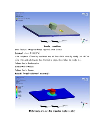


This document summarizes key aspects of friction stir welding (FSW), including: 1) FSW is a solid-state welding process that uses a rotating tool to soften and join two facing workpieces without melting. 2) The document describes tool designs, important welding parameters like rotation speed and travel speed, and the effects on weld quality. 3) It also discusses FSW advantages over fusion welding, including improved mechanical properties and lack of defects like porosity.