FluidDynamics.ppt

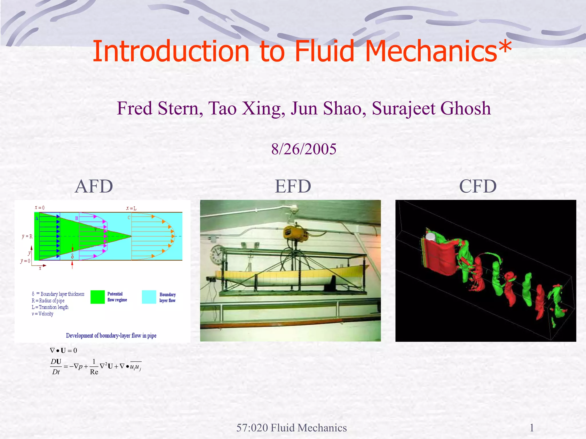
57:020 Fluid Mechanics 1
Introduction to Fluid Mechanics*
CFD
EFD
AFD
2
0
1
Re
i j
D
p u u
Dt
 
    
U
U
U
Fred Stern, Tao Xing, Jun Shao, Surajeet Ghosh
8/26/2005

Fluid Mechanics
• Fluids essential to life
• Human body 65% water
• Earth’s surface is 2/3 water
• Atmosphere extends 17km above the earth’s surface
• History shaped by fluid mechanics
• Geomorphology
• Human migration and civilization
• Modern scientific and mathematical theories and methods
• Warfare
• Affects every part of our lives

History
Faces of Fluid Mechanics
Archimedes
(C. 287-212 BC)
Newton
(1642-1727)
Leibniz
(1646-1716)
Euler
(1707-1783)
Navier
(1785-1836)
Stokes
(1819-1903)
Reynolds
(1842-1912)
Prandtl
(1875-1953)
Bernoulli
(1667-1748)
Taylor
(1886-1975)

Significance
• Fluids omnipresent
• Weather & climate
• Vehicles: automobiles, trains, ships, and
planes, etc.
• Environment
• Physiology and medicine
• Sports & recreation
• Many other examples!

Weather & Climate
Tornadoes
Hurricanes
Global Climate
Thunderstorm

Vehicles
Aircraft
Submarines
High-speed rail
Surface ships

Environment
Air pollution River hydraulics

Physiology and Medicine
Blood pump Ventricular assist device

Sports & Recreation
Water sports
Auto racing
Offshore racing
Cycling
Surfing

Fluids Engineering
2
2
P
B
UD 

2 2
s SM SN
U U U
 
Reality
Fluids Engineering System Components Idealized
EFD, Mathematical Physics Problem Formulation
AFD, CFD,
m
U

Analytical Fluid Dynamics
• The theory of mathematical physics
problem formulation
• Control volume & differential analysis
• Exact solutions only exist for simple
geometry and conditions
• Approximate solutions for practical
applications
• Linear
• Empirical relations using EFD data

• Lecture Part of Fluid Class
• Definition and fluids properties
• Fluid statics
• Fluids in motion
• Continuity, momentum, and energy principles
• Dimensional analysis and similitude
• Surface resistance
• Flow in conduits
• Drag and lift

Schematic
• Example: laminar pipe flow
Exact solution :
2 2
1
( ) ( )( )
4
p
u r R r
x


  

Friction factor:
8
8 64
Re
2 2
w
du
dy
w
f
V V


 
  
Assumptions: Fully developed, Low
Approach: Simplify momentum equation,
integrate, apply boundary conditions to
determine integration constants and use
energy equation to calculate head loss
x
g
y
u
x
u
x
p
Dt
Du
















 2
2
2
2

Head loss:
1 2
1 2 f
p p
z z h
 
   
2
2
32
2
f
L V LV
h f
D g D


 
UD
2000
Re 



0
0
0

• Example: turbulent flow in smooth pipe( )
0 5
y
 
1
ln
u y B

 
  5
20 10
y
 
*
0
1
U u r
f
u r
 

 
 
 
5
10
y

u y
 

    *
0
*
1
ln
u r r r u
B
u  

 
Re 3000

*
y yu 


*
u u u


*
w
u  

Three layer concept (using dimensional analysis)
1. Laminar sub-layer (viscous shear dominates)
2. Overlap layer (viscous and turbulent shear important)
3. Outer layer (turbulent shear dominates)
Assume log-law is valid across entire pipe:
Integration for average velocity and using EFD data to adjust constants:
 
1 2
1
2log Re .8
f
f
 
(k=0.41, B=5.5)

• Example: turbulent flow in rough pipe
 
u u y k
 

1
ln
y
u
k


 
1
2log
3.7
k D
f
 
 
1
ln 8.5 Re
y
u f
k


  
Three regimes of flow depending on k+
1. K+<5, hydraulically smooth (no effect of roughness)
2. 5 < K+< 70, transitional roughness (Re dependent)
3. K+> 70, fully rough (independent Re)
Both laminar sublayer and overlap layer
are affected by roughness
Inner layer:
Outer layer: unaffected
Overlap layer:
Friction factor:
For 3, using EFD data to adjust constants:
constant

• Example: Moody diagram for turbulent pipe flow
1 1 2
2
1 2.51
2log
3.7 Re
k D
f
f
 
  
 
 
Composite Log-Law for smooth and rough pipes is given by the Moody diagram:

Experimental Fluid Dynamics (EFD)
Definition:
Use of experimental methodology and procedures for solving fluids
engineering systems, including full and model scales, large and table
top facilities, measurement systems (instrumentation, data acquisition
and data reduction), uncertainty analysis, and dimensional analysis and
similarity.
EFD philosophy:
• Decisions on conducting experiments are governed by the ability of the
expected test outcome, to achieve the test objectives within allowable
uncertainties.
• Integration of UA into all test phases should be a key part of entire
experimental program
• test design
• determination of error sources
• estimation of uncertainty
• documentation of the results

Purpose
• Science & Technology: understand and investigate a
phenomenon/process, substantiate and validate a theory
(hypothesis)
• Research & Development: document a process/system,
provide benchmark data (standard procedures,
validations), calibrate instruments, equipment, and
facilities
• Industry: design optimization and analysis, provide data
for direct use, product liability, and acceptance
• Teaching: instruction/demonstration

Applications of EFD
Application in research & development
Tropic Wind Tunnel has the ability to create
temperatures ranging from 0 to 165 degrees
Fahrenheit and simulate rain
Application in science & technology
Picture of Karman vortex shedding

Applications of EFD (cont’d)
Example of industrial application
NASA's cryogenic wind tunnel simulates flight
conditions for scale models--a critical tool in
designing airplanes.
Application in teaching
Fluid dynamics laboratory

Full and model scale
• Scales: model, and full-scale
• Selection of the model scale: governed by dimensional analysis and similarity

Measurement systems
• Instrumentation
• Load cell to measure forces and moments
• Pressure transducers
• Pitot tubes
• Hotwire anemometry
• PIV, LDV
• Data acquisition
• Serial port devices
• Desktop PC’s
• Plug-in data acquisition boards
• Data Acquisition software - Labview
• Data analysis and data reduction
• Data reduction equations
• Spectral analysis

Instrumentation
Load cell
Pitot tube
Hotwire 3D - PIV

Data acquisition system
Hardware
Software - Labview

Data reduction methods
EXPERIMEN
RESULT
INDIVIDU
MEASUREM
SYSTEM
MEASUREM
OF INDIVID
VARIABL
DATA REDUC
EQUATIO
TEMPERATURE
WATER
TEMPERATURE
AIR
f
B , P
VENTURI
PRESSURE
PIPE
PRESSURE
f = F( , , z , Q =
  )
a
a
w
g D

8LQ


Q = F( z )

w
w
T
T
B T
, P
z
z
B , P
f f
SM
SM
w
w
DM
SM
2
2
5
a
T
T
B T
, P
a
a
zSM
z
z
B , P
DM
DM zDM
= F(T )


( )
w
= F(T )
a
z
SM i
- z
SM j
w
a
Example of data reduction equations
• Data reduction equations
• Spectral analysis
 
 








 Stat
SM
Stag
SM
a
w
z
r
z
g
r
u


2
)
(

Spectral analysis
FFT: Converts a function from amplitude as function
of time to amplitude as function of frequency
Aim: To analyze the natural
unsteadiness of the separated flow,
around a surface piercing
strut, using FFT.
Fast Fourier Transform
Surface piercing strut Power spectral density
of wave elevation
Free-surface wave
elevation contours
FFT of wave elevation
Time history of wave
elevation

Uncertainty analysis
r = r (X , X ,......, X )
1 2 J
1 2 J
MEASUREMENT
OF INDIVIDUAL
VARIABLES
INDIVIDUAL
MEASUREMENT
SYSTEMS
ELEMENTAL
ERROR SOURCES
DATA REDUCTION
EQUATION
EXPERIMENTAL
RESULT
X
B , P
1
1 1
X
B , P
2
2 2
X
B , P
J
J J
r
B , P
r r
Rigorous methodology for uncertainty assessment
using statistical and engineering concepts

Dimensional analysis
• Definition : Dimensional analysis is a process of formulating fluid mechanics problems in
in terms of non-dimensional variables and parameters.
• Why is it used :
• Reduction in variables ( If F(A1, A2, … , An) = 0, then f(P1, P2, … Pr < n) = 0,
where, F = functional form, Ai = dimensional variables, Pj = non-dimensional
parameters, m = number of important dimensions, n = number of dimensional variables, r
= n – m ). Thereby the number of experiments required to determine f vs. F is reduced.
• Helps in understanding physics
• Useful in data analysis and modeling
• Enables scaling of different physical dimensions and fluid properties
Example
Vortex shedding behind cylinder
Drag = f(V, L, r, m, c, t, e, T, etc.)
From dimensional analysis,
Examples of dimensionless quantities : Reynolds number, Froude
Number, Strouhal number, Euler number, etc.

Similarity and model testing
• Definition : Flow conditions for a model test are completely similar if all relevant
dimensionless parameters have the same corresponding values for model and prototype.
• Pi model = Pi prototype i = 1
• Enables extrapolation from model to full scale
• However, complete similarity usually not possible. Therefore, often it is necessary to
use Re, or Fr, or Ma scaling, i.e., select most important Pand accommodate others
as best possible.
• Types of similarity:
• Geometric Similarity : all body dimensions in all three coordinates have the same
linear-scale ratios.
• Kinematic Similarity : homologous (same relative position) particles lie at homologous
points at homologous times.
• Dynamic Similarity : in addition to the requirements for kinematic similarity the model
and prototype forces must be in a constant ratio.

EFD process
• “EFD process” is the steps to set up an experiment and
take data
Test
Set-up
Facility &
conditions
Install model
Prepare
measurement
systems
Data
Acquisition
Data
Reduction
Uncertainty
Analysis
Data
Analysis
Initialize data
acquisition
software
Run tests &
acquire data
Store data
Statistical
analysis
Estimate bias
limits
Compare results
with benchmark
data, CFD, and
/or AFD
Evaluate fluid
physics
Calibration
Prepare
experimental
procedures
Data reduction
equations
Estimate
precision limits
Estimate total
uncertainty
Prepare report

EFD – “hands on” experience
Lab1: Measurement of density and
kinematic viscosity of a fluid Lab2: Measurement of
flow rate, friction factor and
velocity profiles in smooth and
rough pipes.
Lab3: Measurement of surface pressure
Distribution, lift and drag coefficient for an airfoil
To
Scanivalve
Chord-wise
Pressure
Taps
Tygon
Tubing
Load Cell
Load Cell
L
D

Computational Fluid Dynamics
• CFD is use of computational methods for
solving fluid engineering systems, including
modeling (mathematical & Physics) and
numerical methods (solvers, finite differences,
and grid generations, etc.).
• Rapid growth in CFD technology since advent
of computer
ENIAC 1, 1946 IBM WorkStation

Purpose
• The objective of CFD is to model the continuous fluids
with Partial Differential Equations (PDEs) and
discretize PDEs into an algebra problem, solve it,
validate it and achieve simulation based design
instead of “build & test”
• Simulation of physical fluid phenomena that are
difficult to be measured by experiments: scale
simulations (full-scale ships, airplanes), hazards
(explosions,radiations,pollution), physics (weather
prediction, planetary boundary layer, stellar evolution).

Modeling
• Mathematical physics problem formulation of fluid
engineering system
• Governing equations: Navier-Stokes equations (momentum),
continuity equation, pressure Poisson equation, energy
equation, ideal gas law, combustions (chemical reaction
equation), multi-phase flows(e.g. Rayleigh equation), and
turbulent models (RANS, LES, DES).
• Coordinates: Cartesian, cylindrical and spherical coordinates
result in different form of governing equations
• Initial conditions(initial guess of the solution) and Boundary
Conditions (no-slip wall, free-surface, zero-gradient,
symmetry, velocity/pressure inlet/outlet)
• Flow conditions: Geometry approximation, domain, Reynolds
Number, and Mach Number, etc.

Modeling (examples)
Free surface animation for ship in
regular waves
Developing flame surface (Bell et al., 2001)
Evolution of a 2D mixing layer laden with particles of Stokes
Number 0.3 with respect to the vortex time scale (C.Narayanan)

Modeling (examples, cont’d)
3D vortex shedding behind a circular cylinder
(Re=100,DNS,J.Dijkstra)
DES,
Re=105, Iso-
surface of Q
criterion (0.4)
for turbulent
flow around
NACA12 with
angle of attack
60 degrees
LES of a turbulent jet. Back wall shows a slice of the dissipation rate and the
bottom wall shows a carpet plot of the mixture fraction in a slice through the jet
centerline, Re=21,000 (D. Glaze).

Numerical methods
• Finite difference methods:
using numerical scheme to
approximate the exact derivatives
in the PDEs
• Finite volume methods
• Grid generation: conformal
mapping, algebraic methods and
differential equation methods
• Grid types: structured,
unstructured
• Solvers: direct methods (Cramer’s
rule, Gauss elimination, LU
decomposition) and iterative
methods (Jacobi, Gauss-Seidel,
SOR)
Slice of 3D mesh of a fighter aircraft
o x
y
i i+1
i-1
j+1
j
j-1
imax
jmax
x

y

2
1 1
2 2
2
i i i
P P P
P
x x
 
 


 
2
1 1
2 2
2
j j j
P P P
P
y y
 
 


 

CFD process
Viscous Model
Boundary
Conditions
Initial
Conditions
Convergent
Limit
Contours
Precisions
(single/
double)
Numerical
Scheme
Vectors
Streamlines
Verification
Geometry
Select
Geometry
Geometry
Parameters
Physics Mesh Solve Post-
Processing
Compressible
ON/OFF
Flow
properties
Unstructured
(automatic/
manual)
Steady/
Unsteady
Forces Report
(lift/drag, shear
stress, etc)
XY Plot
Domain Shape
and Size
Heat Transfer
ON/OFF
Structured
(automatic/
manual)
Iterations/
Steps
Validation
Reports

Commercial software
• CFD software
1. FLUENT: http://www.fluent.com
2. FLOWLAB: http://www.flowlab.fluent.com
3. CFDRC: http://www.cfdrc.com
4. STAR-CD: http://www.cd-adapco.com
5. CFX/AEA: http://www.software.aeat.com/cfx
• Grid Generation software
1. Gridgen: http://www.pointwise.com
2. GridPro: http://www.gridpro.com
• Visualization software
1. Tecplot: http://www.amtec.com
2. Fieldview: http://www.ilight.com

“Hands-on” experience using CFD
Educational Interface (pipe template)

“Hands-on” experience using CFD
Educational Interface (airfoil template)

57:020 Fluid Mechanics
• Lectures cover basic concepts in fluid statics,
kinematics, and dynamics, control-volume, and
differential-equation analysis methods. Homework
assignments, tests, and complementary EFD/CFD
labs
• This class provides an introduction to all three tools:
AFD through lecture and CFD and EFD through labs
• ISTUE Teaching Modules
(http://www.iihr.uiowa.edu/~istue) (next two slides)

TM Descriptions
http://css.engineering.uiowa.edu/~fluids
Table 1: ISTUE Teaching Modules for Introductory Level Fluid Mechanics at Iowa
Teaching Modules TM for Fluid
Property
TM for Pipe Flow TM for Airfoil Flow
Overall Purpose Hands-on student
experience with table-top
facility and simple MS for
fluid property
measurement, including
comparison manufacturer
values and rigorous
implementation standard
EFD UA
Hands-on student experience
with complementary EFD, CFD,
and UA for Introductory Pipe
Flow, including friction factor
and mean velocity measurements
and comparisons benchmark
data, laminar and turbulent flow
CFD simulations, modeling and
verification studies, and
validation using AFD and EFD.
Hands-on student experience with
complementary EFD, CFD, and UA
for Introductory Airfoil Flow,
including lift and drag, surface
pressure, and mean and turbulent
wake velocity profile measurements
and comparisons benchmark data,
inviscid and turbulent flow
simulations, modeling and verification
studies, and validation using AFD and
EFD.
Educational Materials FM and EFD lecture; lab
report instructions; pre lab
questions, and EFD
exercise notes.
FM, EFD and CFD lectures; lab
report instructions; pre lab
questions, and EFD and CFD
exercise notes.
FM, EFD and CFD lectures; lab
report instructions; pre lab questions,
and EFD and CFD exercise notes.
ISTUE ASEE papers Paper 1 Paper2
FM Lecture Introduction to Fluid Mechanics
Lab Report Instructions EFD lab report Instructions CFD lab report Instructions
Continued in next slide…

TM Descriptions, cont’d
Teaching Modules TM for Fluid
Property
TM for Pipe Flow TM for Airfoil Flow
CFD CFD Lecture Introduction to CFD
Exercise Notes None CFD Prelab1
PreLab1 Questions
CFD Lab 1
Lab Concepts
EFD Data
CFD Prelab2
PreLab 2 Questions
CFD Lab2
Lab Concepts
EFD Data
EFD EFD
Lecture
EFD and UA
Exercise Notes PreLab1 Questions
Lab1 Lecture
Lab 1 exercise notes
Lab 1 data
reduction sheet
Lab concepts
PreLab2 Questions
Lab2 Lecture
Lab2 Data reduction
sheet (smooth & rough)
Lab concepts
PreLab3 Questions
Lab3 Lecture
Data Reduction Sheet
Lab concepts
UA(EFD) Lecture EFD UA Report
Exercise Notes Instructions UA
UA(CFD) Lecture
Exercise Notes None

FluidDynamics.ppt

More Related Content

What's hot

Similar to FluidDynamics.ppt

Recently uploaded

FluidDynamics.ppt