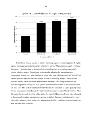
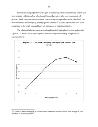
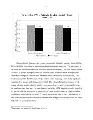
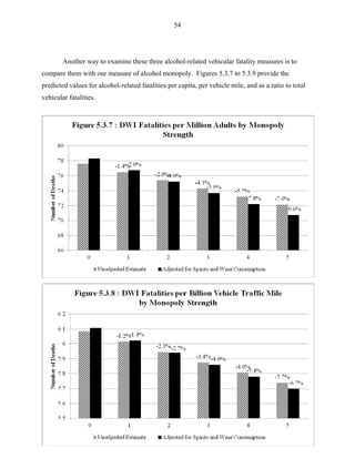
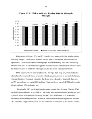
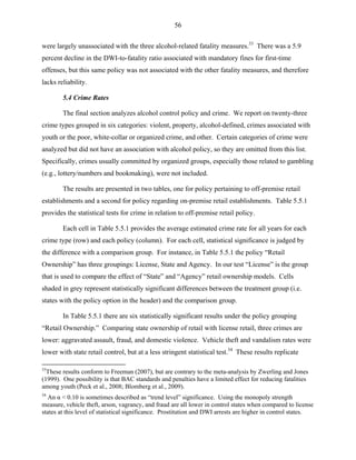
Download to read offline

![7
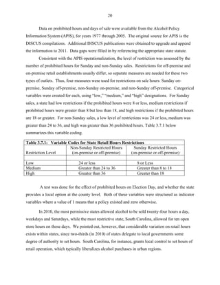
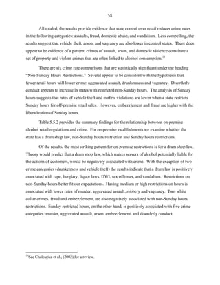
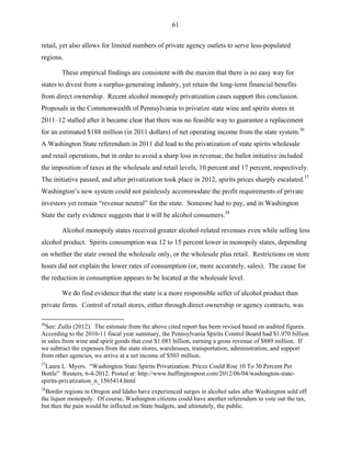
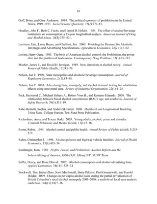
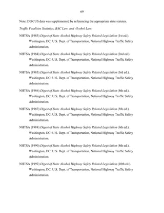
Agency,9
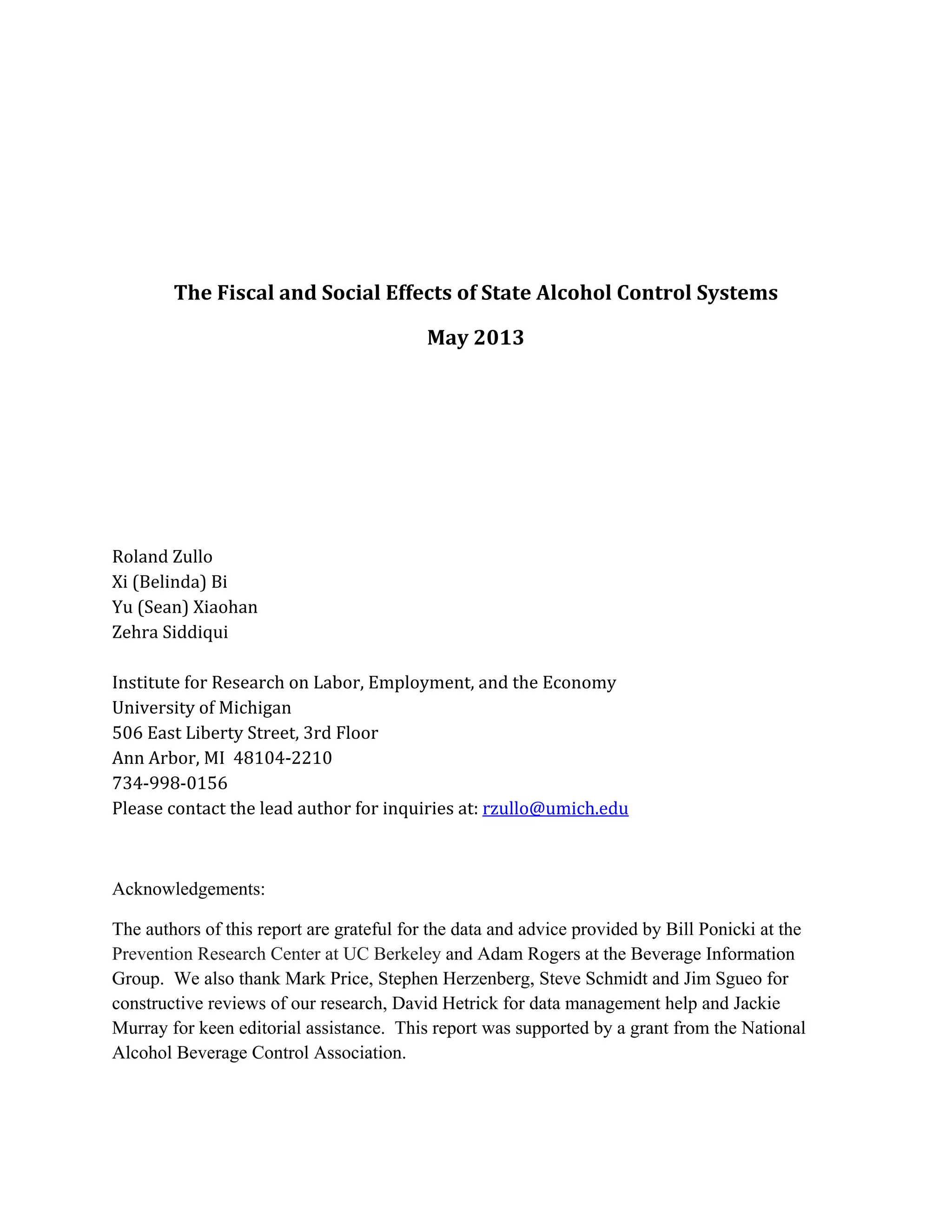
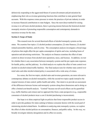
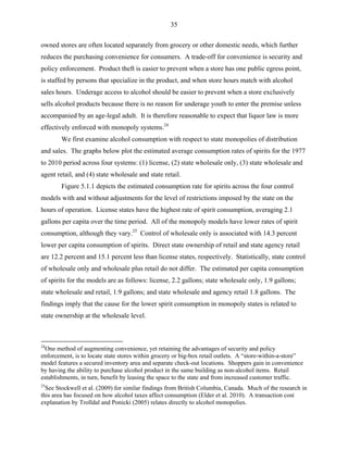
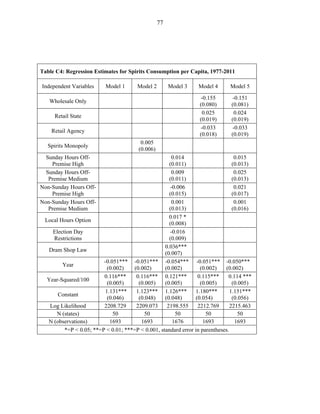
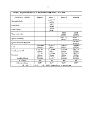
Agency Only, and License. The composite measures, Spirits Monopoly and Wine
Monopoly, each have six possible values, from 0 to 5, where 0 is a license state and 5 represents
state-owned wholesale and retail. Values for these variables were assigned based on the matrix
in Table 3.3.1. Evident from the counts in the table is the variation in retail arrangements, which
in recent history has been the main area of state divestment.
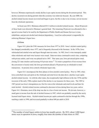
Table 3.1.1: Monopoly Strength Measure
Wholesale Ownership and Control
State Only Private Agent Private License
RetailOwnershipandControl
State Only
5
(303)
[50]
4
(N/O)
[N/O]
3
(N/O)
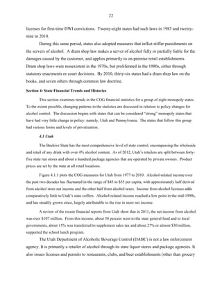
[8]
State and Private Agent
4
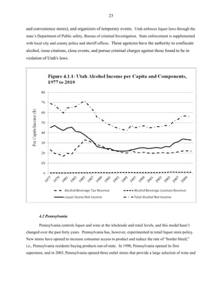
(116)
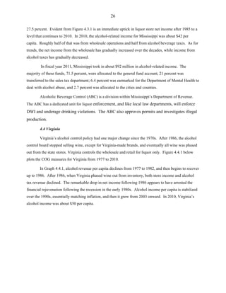
[35]
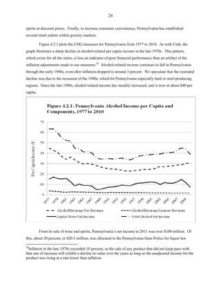
3
(N/O)
[N/O]
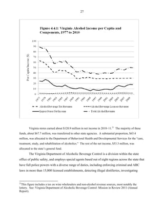
2
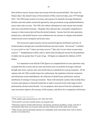
(N/O)
[N/O]
Private Agent Only
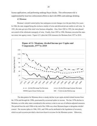
3
(63)1
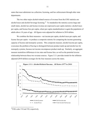
[N/O]
2
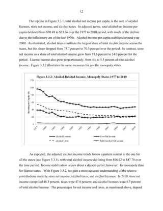
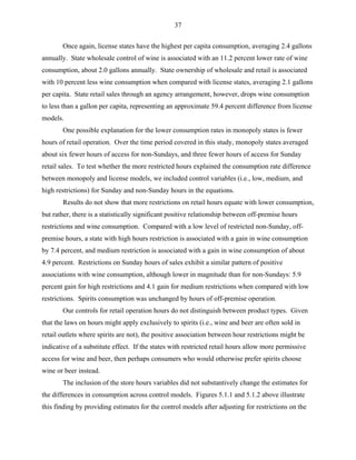
(7)
[N/O]
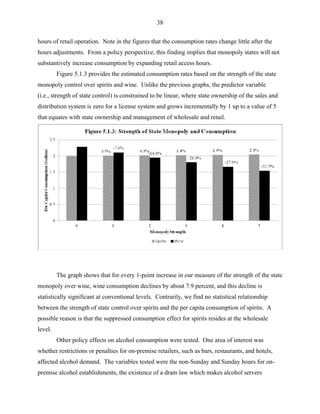
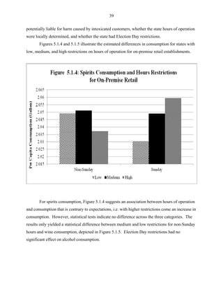
1
(N/O)
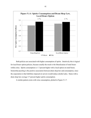
[37]3
Private License
2
(142)
[120]2
1
(N/O)
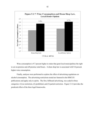
[N/O]
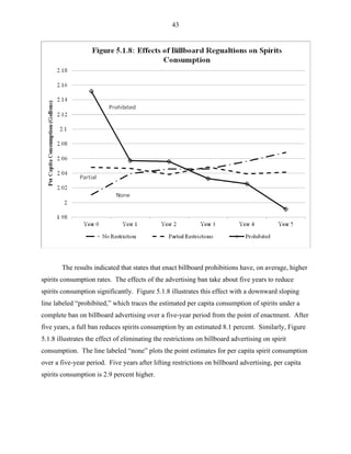
0
(1,120)
[1,501]
For each cell: the top number is the assigned variable score for monopoly strength,
the second number (in parentheses) is the number of observations for spirits, and the
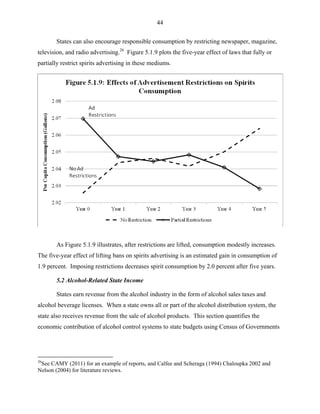
third number [in brackets] is the number of observations for wine. N/O indicates no
observations.
1
Includes 5 observations where a state was transitioning from public to private license, and
therefore had both types of retail stores.
2
Includes 45 observations where the state stores carried a limited number of wine products
as they phased out wine inventory.
3
All 37 observations are where the state retail stores held wine inventory during a transition
to private license.
9
States with both types of stores usually place state-owned stores in high traffic areas and agency stores
in less populated regions.](https://image.slidesharecdn.com/4c3a2046-1bd4-4f72-ba13-2376441782e9-150602012944-lva1-app6891/85/FiscalAndSocialEffectsOfStateAlcoholControlSystems-12-320.jpg)
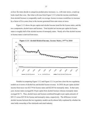
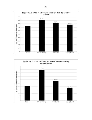
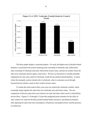
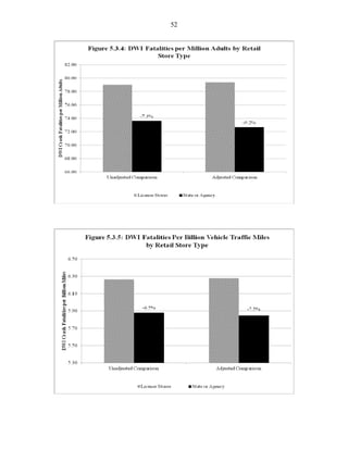


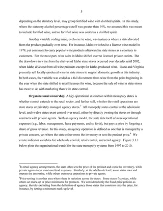
This document summarizes a study examining the fiscal and social effects of state alcohol control systems in the United States. It analyzes data from the late 1970s to 2010 comparing states with alcohol monopolies to those with private license systems. Key findings include: 1) States with alcohol monopolies had lower spirits and wine consumption on average. Restricting alcohol advertising was also associated with lower consumption. 2) Alcohol monopolies generated substantially higher alcohol-related tax revenues for states than private systems. Wholesale monopolies provided the largest financial gain. 3) Alcohol monopolies were associated with lower alcohol-related traffic fatality and crime rates for some offenses like assaults and vandalism compared to license states.


