Download the fullversion and explore a variety of test banks
or solution manuals at https://testbankdeal.com
Financial Statement Analysis 11th Edition
Subramanyam Solutions Manual
_____ Tap the link below to start your download _____
https://testbankdeal.com/product/financial-statement-
analysis-11th-edition-subramanyam-solutions-manual/
Find test banks or solution manuals at testbankdeal.com today!
2.
We believe theseproducts will be a great fit for you. Click
the link to download now, or visit testbankdeal.com
to discover even more!
Financial Statement Analysis 11th Edition Subramanyam Test
Bank
https://testbankdeal.com/product/financial-statement-analysis-11th-
edition-subramanyam-test-bank/
Financial Statement Analysis 10th Edition Subramanyam Test
Bank
https://testbankdeal.com/product/financial-statement-analysis-10th-
edition-subramanyam-test-bank/
Financial Statement Analysis International Edition 13th
Edition Gibson Solutions Manual
https://testbankdeal.com/product/financial-statement-analysis-
international-edition-13th-edition-gibson-solutions-manual/
Andersons Business Law and the Legal Environment Standard
Volume 22nd Edition Twomey Test Bank
https://testbankdeal.com/product/andersons-business-law-and-the-legal-
environment-standard-volume-22nd-edition-twomey-test-bank/
3.
Principles of EnvironmentalScience Inquiry and
Applications 7th Edition Cunningham Test Bank
https://testbankdeal.com/product/principles-of-environmental-science-
inquiry-and-applications-7th-edition-cunningham-test-bank/
Understanding American Government 14th Edition Welch Test
Bank
https://testbankdeal.com/product/understanding-american-
government-14th-edition-welch-test-bank/
Physics for Scientists and Engineers 9th Edition Serway
Solutions Manual
https://testbankdeal.com/product/physics-for-scientists-and-
engineers-9th-edition-serway-solutions-manual/
Business Communication Building Critical Skills 6th
Edition Locker Test Bank
https://testbankdeal.com/product/business-communication-building-
critical-skills-6th-edition-locker-test-bank/
Sexuality Now Embracing Diversity 5th Edition Carroll Test
Bank
https://testbankdeal.com/product/sexuality-now-embracing-
diversity-5th-edition-carroll-test-bank/
4.
Organizational Behavior KeyConcepts Skills and Best
Practices 5th Edition Kinicki Solutions Manual
https://testbankdeal.com/product/organizational-behavior-key-concepts-
skills-and-best-practices-5th-edition-kinicki-solutions-manual/
112
[that both thelight and dark markings are of planetary scale]
suggests that they must be related.”
Ed Stone speculated about the other two Galilean satellites.
Ganymede and Callisto are essentially identical in size, mass, and
probably composition. By examining them, we can perhaps learn
what happens when bodies with very similar chemistry have different
“life histories” and different surface properties (there are indications
that Ganymede’s crust may not have been as rigid as Callisto’s).
Going further, he added that Callisto and Mercury, the least dense
and the most dense, respectively, of the terrestrial-style planets,
although totally different in composition and density, seem to have
similar surfaces and similar histories. What would have happened to
Mercury if it had been made of ice, water, and rock as Callisto is?
Would it have evolved as Callisto did?
One of the most spectacular of the Voyager 2 images was obtained from
inside the shadow of Jupiter. Looking back toward the planet and the
rings with its wide-angle camera, the spacecraft took these photos on
July 10 from a distance of 1.5 million kilometers. The ribbon-like nature
of the rings is clearly shown. The planet is outlined by sunlight scattered
37.
from a hazelayer high in the atmosphere. On each side, the arms of the
ring curving back toward the spacecraft are cut off by the planet’s
shadow as they approach the brightly outlined disk. [P-21774B/W]
The rings of Jupiter proved to be unexpectedly bright when seen with the
Sun nearly behind them. Strong forward scattering of sunlight is
characteristic of small particles. These two views were obtained by
Voyager 2 on July 10 from a perspective inside the shadow of Jupiter.
The distance of the spacecraft from the rings was about 1.5 million
kilometers. Although the resolution has been degraded by camera motion
during the time exposures, these images reveal that the rings have some
radial structure. [260-610B/W and 260-674]
38.
HIGHLIGHTS OF THEVOYAGER 2 SCIENTIFIC FINDINGS
[3]
Atmosphere
The main atmospheric jet streams were present during both
Voyager encounters, with some changes in velocity.
39.
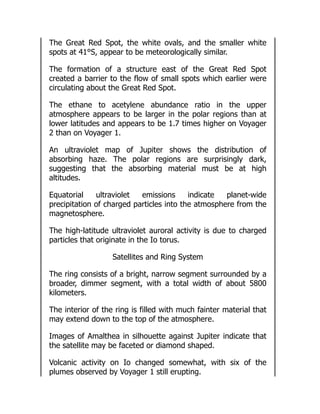
The Great RedSpot, the white ovals, and the smaller white
spots at 41°S, appear to be meteorologically similar.
The formation of a structure east of the Great Red Spot
created a barrier to the flow of small spots which earlier were
circulating about the Great Red Spot.
The ethane to acetylene abundance ratio in the upper
atmosphere appears to be larger in the polar regions than at
lower latitudes and appears to be 1.7 times higher on Voyager
2 than on Voyager 1.
An ultraviolet map of Jupiter shows the distribution of
absorbing haze. The polar regions are surprisingly dark,
suggesting that the absorbing material must be at high
altitudes.
Equatorial ultraviolet emissions indicate planet-wide
precipitation of charged particles into the atmosphere from the
magnetosphere.
The high-latitude ultraviolet auroral activity is due to charged
particles that originate in the Io torus.
Satellites and Ring System
The ring consists of a bright, narrow segment surrounded by a
broader, dimmer segment, with a total width of about 5800
kilometers.
The interior of the ring is filled with much fainter material that
may extend down to the top of the atmosphere.
Images of Amalthea in silhouette against Jupiter indicate that
the satellite may be faceted or diamond shaped.
Volcanic activity on Io changed somewhat, with six of the
plumes observed by Voyager 1 still erupting.
40.
The largest Voyager1 plume (Pele) had ceased, while the
dimensions of another plume (Loki) had increased by 50
percent.
Several large-scale changes in Io’s appearance had occurred,
consistent with surface deposition rates calculated for the large
eruptions.
Europa is remarkably smooth with very few craters. The
surface consists primarily of uniformly bright terrain crossed by
linear markings and very low ridges.
There are four basic terrain types on Ganymede, including
younger, smooth terrain and a rugged impact basin first
observed by Voyager 2.
Callisto’s entire surface is densely cratered and is likely to be
several billion years old.
Equatorial surface temperatures on the Galilean satellites range
from 80 K (night) to 155 K (the subsolar point on Callisto).
Magnetosphere
The outer region of the magnetosphere contains a hot plasma
consisting primarily of hydrogen, oxygen, and sulfur ions.
The hot plasma generally flows in the corotation direction out
to the boundary of the magnetosphere.
Beyond about 160 RJ, the hot plasma streams nearly
antisunward.
Outbound the spacecraft experienced multiple magnetopause
crossings between 204 RJ and 215 RJ.
41.
114
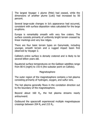
The abundance ofoxygen and sulfur relative to helium at high
energy increases with decreasing distance from Jupiter.
Measurements of high energy oxygen suggest that these nuclei
are diffusing inward toward Jupiter.
The ultraviolet emission from the Io plasma torus was twice as
bright as four months earlier and the temperature had
decreased by 30 percent to 60 000 K.
The low-frequency (kilometric) radio emissions from Jupiter
have a strong latitude dependence and often contain
narrowband emissions that drift to lower or higher frequencies
with time.
A complex magnetospheric interaction with Ganymede was
observed in the magnetic field, plasma, and energetic particles
up to about 200 000 kilometers from the satellite.
[3]
Adapted from a summary prepared by E. C. Stone and A. L.
Lane for the Voyager 2 Thirty-Day Report.
A new inner satellite of Jupiter, provisionally designated 1979J1, was
discovered by David Jewitt and Ed Danielson of Caltech in these Voyager
2 ring photographs.
42.
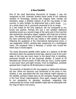
In a 15-secondexposure with the wide-angle camera, the edge-on ring
shows as a faint line, and the satellite is the dot indicated by the arrow.
[260-807]
In a narrow angle 96-second exposure, the motion of the satellite can be
seen. Again, the faint band is the ring, blurred by camera motion, and the
arrow indicates the streak due to the satellite. A star streak is located
above and to the left of the satellite; note that the length and angle of
the two trails are different, owing to satellite motion. [P-22172]
43.
115
A New Satellite
Oneof the most fascinating discoveries of Voyager 2 was not
recognized at first. Graduate student David Jewitt of the California
Institute of Technology, working with Imaging Team member Ed
Danielson, began a detailed analysis of all the ring photos in late
summer. In early October he determined that a short streak
on a photo taken July 8, previously presumed to be an image
of a star trailed by the time exposure, did not correspond to any
known star position. Perhaps this was a new satellite! Additional
sleuthing turned up a second image of the same part of the ring that
also showed the anomalous object, together with trails due to known
stars. The differing angles and lengths of the trails of the object and
the stars confirmed that this was indeed a 14th satellite of Jupiter.
Following the guidelines of the International Astronomical Union, it
was designated 1979J1, pending later assignment of a mythological
name. The proposed name is Adrastea, a nymph who nursed the
infant Zeus in Greek legend.
The newly discovered satellite orbits Jupiter at a distance of 58 000
kilometers above the equatorial cloud tops, placing it just at the outer
edge of the ring and much closer to the planet than is Amalthea,
previously thought to be the innermost satellite. It travels at 30
kilometers per second (nearly 70 000 miles per hour), circling Jupiter
in just seven hours and eight minutes. From its brightness, scientists
guessed that it might be 30-40 kilometers in diameter.
The proximity of Adrastea to the ring suggests a relationship between
the two. When the discovery was announced to the press in mid-
October, it was speculated that the ring material might originate on
the satellite, perhaps eroded away by the energetic charged particles
in the inner Jovian magnetosphere. Once again, Voyager had added
to our perspective on planetary processes, suggesting that
undiscovered but similar small satellites might also be associated with
the rings of Saturn and Uranus.
44.
Voyager 2 hadcertainly added a few years’ of data of its own to
Voyager 1’s “ten years’ worth of data.” It had given a different view of
the Jovian system, helping to solve some of the mystery surrounding
Jupiter and its satellites, and creating new mysteries. As Voyager 2
sped out away from Jupiter, riding along the giant planet’s huge
magnetotail, attention turned to Saturn: What would Pioneer 11, the
Pathfinder, discover in September 1979? What would the Voyagers
learn in November 1980 and August 1981? Would all go well? Would
Voyager 2 fly on to Uranus?
There was also a yearning to examine more closely, with the Galileo
Project, what had been unknown for so long, yet had become so
familiar in only a few months’ time—the little dark, red “potato”
Amalthea, the volcano-covered world Io, the mysterious “cracked
billiard ball” Europa, cratered and groovy Ganymede, ancient Callisto,
and the king of the planets itself, a colorful, banded world of stable
climate and ever-changing weather patterns.
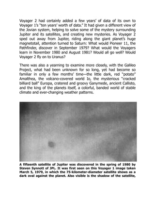
A fifteenth satellite of Jupiter was discovered in the spring of 1980 by
Steven Synnott of JPL. It was first seen on this Voyager 1 image taken
March 5, 1979, in which the 75-kilometer-diameter satellite shows as a
dark oval against the planet. Also visible is the shadow of the satellite,
45.
116
designated 1979J2. Thissatellite orbits between Io and Amalthea with a
period of 16 hours and 11 minutes. [P-22580B/W]
46.
117
The Jupiter seenby the Voyager cameras is a cloud-belted world of rapid
jet streams and complex cloud forms. Prominent in this Voyager 1 image,
taken February 5 at a range of 28.4 million kilometers, is the alternating
structure of light zones and dark belts, and the Great Red Spot and
numerous smaller spots. Also easily visible are the two inner Galilean
satellites, Io and Europa. The resolution in this picture is 500 kilometers,
about five times better than can be obtained from Earth-based
telescopes. Callisto can be faintly seen at the lower left. [P-21083C]
47.
CHAPTER 8
JUPITER—KING OFTHE PLANETS
A Star That Failed
More massive than all the other planets combined, Jupiter dominates
the planetary system. The giant revealed by Voyager is a gas planet
of great complexity; its atmosphere is in constant motion, driven by
heat escaping from a glowing interior as well as by sunlight absorbed
from above. Energetic atomic particles stream around it, caught in a
magnetic field that reaches out nearly 10 million kilometers into the
surrounding space, embracing the seven inner satellites. From its
deep interior through its seething clouds out to its pulsating
magnetosphere, Jupiter is a place where forces of incredible energy
contend.
At its birth, Jupiter shone like a star. The energy released by infalling
material from the solar nebula heated its interior, and the larger it
grew the hotter it became. Theorists calculate that when the nebular
material was finally exhausted, Jupiter had a diameter more than ten
times its present one, a central temperature of about 50 000 K, and a
luminosity about one percent as great as that of the Sun today.
At this early stage, Jupiter rivaled the Sun. Had it been perhaps 70
times more massive than it was, it would have continued to contract
and increase in temperature, until self-sustaining nuclear reactions
could ignite in its interior. If this had happened, the Sun would have
been a double star, and the Earth and the other planets might not
have formed. However, Jupiter did not make it as a star; after a brief
flash of glory, it began to cool.
48.
118
At first Jupitercontinued to collapse. Within the first ten million years
of its life, the planet was reduced to nearly its present size, with only
a few percent additional shrinkage during the past 4.5 billion years.
The luminosity also dropped as internal heat was carried to the
surface by convection and radiated away to space. After a million
years Jupiter emitted only one-hundred thousandth as much radiation
as the Sun, and today its luminosity is only one-ten billionth of the
Sun’s.
Jupiter’s internal energy, although small by stellar standards, has
important effects on the planet. About 10¹⁷ watts of power,
comparable to that received by Jupiter from the Sun, reach the
surface from the still-luminous interior. The central temperature is still
thought to be about 30 000 K, sufficient to maintain the interior in a
molten state. Scientists generally agree that Jupiter is an entirely fluid
planet, with no solid core whatever.
Composition and Atmospheric Structure
Because of its great mass, Jupiter has been undiscriminating in its
composition. All gases and solids available in the early solar nebula
were attracted and held by its powerful gravity. Thus it is expected
that Jupiter has the same basic composition as the Sun, with both
bodies preserving a sample of the original cosmic material from which
the solar system formed.
49.
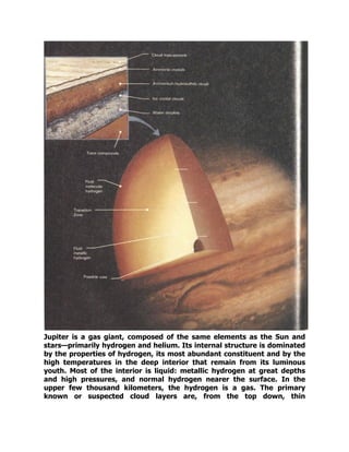
Jupiter is agas giant, composed of the same elements as the Sun and
stars—primarily hydrogen and helium. Its internal structure is dominated
by the properties of hydrogen, its most abundant constituent and by the
high temperatures in the deep interior that remain from its luminous
youth. Most of the interior is liquid: metallic hydrogen at great depths
and high pressures, and normal hydrogen nearer the surface. In the
upper few thousand kilometers, the hydrogen is a gas. The primary
known or suspected cloud layers are, from the top down, thin
50.
119
hydrocarbon “smog”; ammonia;ammonium hydrosulfide; water-ice, and
liquid water. [260-828]
Cloud top-aerosols
Ammonia crystals
Ammonium hydrosulfide clouds
Ice crystal clouds
Water droplets
Trace compounds
Fluid molecular hydrogen
Transition Zone
Fluid metallic hydrogen
Possible core
The primary constituents of Jupiter have long been suspected
to be hydrogen and helium, the two simplest and lightest
atoms. However, it has proved impossible to derive accurate
measurements of the abundance of these two elements from
astronomical observations. On the basis of a rather simple infrared
measurement, Pioneer investigators found He/H₂ = 0.14 ± 0.08. On
Voyager, IRIS was able to obtain much improved infrared spectra,
yielding an initial value of He/H₂ = 0.11 ± 0.3. Voyager scientists
expect that further analysis will reduce the uncertainty to about ±
0.01. The ratio of 0.11 is in excellent agreement with the solar value
of about 0.12, supporting the idea that Jupiter and the Sun have
similar elemental compositions.
Astronomers have known for a long time that, in addition to
hydrogen and helium, the compounds methane (CH₄) and ammonia
(NH₃) are present in the visible atmosphere of Jupiter. In the 1970s,
additional spectra in the infrared resulted in the discovery of water
(H₂O), ethane (C₂H₆), germane (GeH₄), acetylene (C₂H₂), phosphine
(PH₃), carbon monoxide (CO), hydrogen cyanide (HCN), and carbon
dioxide (CO₂). All these are trace constituents, with two of them,
ethane and acetylene, apparently formed at high altitudes by the
action of sunlight on methane.
51.
A total ofapproximately 100 000 infrared spectra, many of small
regions on the disk, were obtained by IRIS. These spectra generally
show hydrogen, helium, methane, ammonia, phosphine, ethane, and
acetylene. In addition, excellent spectra were obtained in “hot spots,”
regions in which breaks in the upper clouds permit radiation from
deeper layers to escape. (The hot spots generally correspond to dark
brown regions on photographs of the planet.) IRIS measured
temperatures in the hot spots up to -13° C but no higher; apparently
this temperature corresponds to the top of a deeper cloud deck.
Spectral features indicative of the presence of water vapor and
germane were clearly seen in the hot spots.
Further analysis of the IRIS spectra will be required to derive the
abundances of the gases detected. However, even the preliminary
data showed how variable Jupiter can be, especially in its upper
atmosphere. The two hydrocarbons, ethane and acetylene, vary in
relative abundance with latitude; there is less acetylene near the
poles. In addition to this planetwide trend, smaller variations were
seen from place to place and between the observations in March and
July. All the variations will eventually provide information on the
processes of formation, transportation, and destruction of
hydrocarbons in the upper atmosphere.
ELEMENTS DETECTED IN THE JOVIAN MAGNETOSPHERE
Element Atomic Number Instruments
Hydrogen (H) 1 UVS, Plasma, LECP, CRS
Helium (He) 2 Plasma, LECP
Carbon (C) 6 LECP
Nitrogen (N) 7 CRS
Oxygen (O) 8 UVS, Plasma, LECP, CRS
Neon (Ne) 10 CRS
Sodium (Na) 11 LECP, CRS
Magnesium (Mg) 12 CRS
Silicon (Si) 14 CRS
52.
120
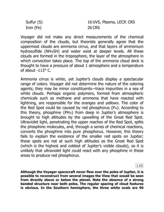
Sulfur (S) 16UVS, Plasma, LECP, CRS
Iron (Fe) 26 CRS
Voyager did not make any direct measurements of the chemical
composition of the clouds, but theorists generally agree that the
uppermost clouds are ammonia cirrus, and that layers of ammonium
hydrosulfide (NH₄SH) and water exist at deeper levels. All these
clouds are formed in the troposphere, the layer of the atmosphere in
which convection takes place. The top of the ammonia cloud deck is
thought to have a pressure of about 1 atmosphere and a temperature
of about -113° C.
Ammonia cirrus is white, yet Jupiter’s clouds display a spectacular
range of colors. Voyager did not determine the nature of the coloring
agents; they may be minor constituents—trace impurities in a sea of
white clouds. Perhaps organic polymers, formed from atmospheric
chemicals such as methane and ammonia that have reacted with
lightning, are responsible for the oranges and yellows. The color of
the Red Spot could be caused by red phosphorus (P₄). According to
this theory, phosphine (PH₃) from deep in Jupiter’s atmosphere is
brought to high altitudes by the upwelling of the Great Red Spot.
Ultraviolet light, penetrating the upper reaches of the Red Spot, splits
the phosphine molecules, and, through a series of chemical reactions,
converts the phosphine into pure phosphorus. However, this theory
fails to explain the existence of the smaller red spots on Jupiter;
these spots are not at such high altitudes as the Great Red Spot
(which is the highest and coldest of Jupiter’s visible clouds), so it is
unlikely that ultraviolet light could react with any phosphine in these
areas to produce red phosphorus.
Although the Voyager spacecraft never flew over the poles of Jupiter, it is
possible to reconstruct from several images the View that would be seen
from directly above or below the planet. Note the absence of a strong
banded structure near both poles. The regular spacing of cloud features
is obvious. In the Southern hemisphere, the three white ovals are 90
53.
degrees apart inlongitude, but a fourth oval at the other quadrant is
missing. The irregular black areas at each pole are places for which no
Voyager data exist. The resolution of the original pictures from which
these polar projections were made was about 600 kilometers.
North pole. [P-21638C]
54.
121
122
South pole. [P-21639C]
Variousforms of elemental sulfur might be responsible for the
riot of color we see on Jupiter. Sulfur forms polymers (S₃, S₄,
S₅, S₈,) that are yellow, red, and brown, but no sulfur in any form
has been detected on Jupiter. “We never promised you we were
55.
going to identifythe colors on Jupiter with this mission,” one of the
atmospheric scientists remarked, “but we will have a probe that is
going into the atmosphere in the mid-1980s—Galileo.” Perhaps the
mystery of the Jovian clouds will have to wait till then.
Temperature maps of Jupiter were obtained by IRIS in radiation
arising at different levels above the clouds. Maps show temperatures
at pressures of 0.8 atmosphere near the clouds, and 0.2 atmosphere
near the top of the troposphere. In addition to the low temperatures
over the bright zones and the higher temperatures over dark belts,
there is a great deal of smaller scale structure. It is interesting that a
cold area corresponding to the Great Red Spot is clearly visible even
near the top of the troposphere, indicating that this feature disturbs
the atmosphere to very high altitudes.
The structure of the atmosphere of Jupiter above the troposphere
was investigated through the radio occultation experiment as well as
by IRIS. The level in which the minimum temperature of about -173°
C occurs has a pressure of 0.1 atmosphere. Above this point lies the
stratosphere, in which temperatures increase with altitude as a result
of sunlight absorbed by the gas or by aerosol particles resembling
smog. At 70 kilometers above the ammonia clouds, the temperature
is about -113° C. Above this level, the temperature stays
approximately constant, although at extreme altitudes the
temperature again rises in the ionosphere.
If one could “unwrap” Jupiter like a map, views such as these would be
obtained. The comparison between the pictures shows the relative
motions of features in Jupiter’s atmosphere. It can be seen, for example,
that the Great Red Spot moved westward and the white ovals eastward
during the time between the acquisition of these pictures. Regular plume
patterns are equidistant around the northern edge of the equator, while a
train of small spots moved eastward at approximately latitude 80° S. In
addition to these relative motions, significant changes are evident in the
recirculating flow east of the Great Red Spot, in the disturbed region
west of the Great Red Spot, and as seen in the brightening of material
spreading into the equatorial region from the more southerly latitudes.
[P-21771C]
56.
123
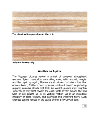
The planet asit appeared about March 1.
As it was in early July.
Weather on Jupiter
The Voyager pictures reveal a planet of complex atmospheric
motions. Spots chase after each other, meet, whirl around, mingle,
and then split up again; filamentary structures curl into spirals that
open outward; feathery cloud systems reach out toward neighboring
regions; cumulus clouds that look like ostrich plumes may brighten
suddenly as they float toward the east; spots stream around the Red
Spot or get caught up in its vortical motion—all in an incredible
interplay of color, texture, and eastward and westward flows. Such
changes can be noticed in the space of only a few Jovian days.
57.
Differing characteristics ofJupiter’s meteorology are apparent in high-
resolution images, such as this one taken by Voyager 1 on March 2 at a
range of 4 million kilometers. The well-defined pale orange line running
from southwest to northeast (north is at the top) marks the high-speed
north temperate current with wind speeds of about 120 meters per
second. Toward the top of the picture, a weaker jet of approximately 30
meters per second is characterized by wave patterns and cloud features
which have been observed to rotate in a clockwise manner at these
latitudes of about 35°N. These clouds have been observed to have
lifetimes of one to two years. [P-21193C]
On a broader time scale, greater changes on the face of Jupiter can
be seen. Features drift around the planet; even the large white ovals
and the Great Red Spot slide along in their respective latitudes. Belts
58.
124
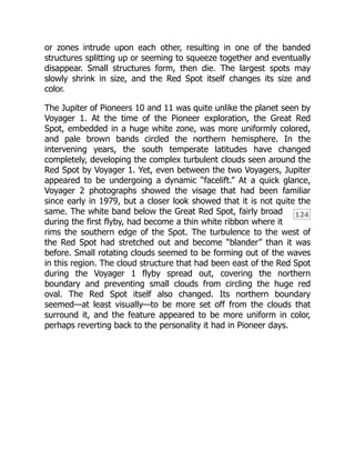
or zones intrudeupon each other, resulting in one of the banded
structures splitting up or seeming to squeeze together and eventually
disappear. Small structures form, then die. The largest spots may
slowly shrink in size, and the Red Spot itself changes its size and
color.
The Jupiter of Pioneers 10 and 11 was quite unlike the planet seen by
Voyager 1. At the time of the Pioneer exploration, the Great Red
Spot, embedded in a huge white zone, was more uniformly colored,
and pale brown bands circled the northern hemisphere. In the
intervening years, the south temperate latitudes have changed
completely, developing the complex turbulent clouds seen around the
Red Spot by Voyager 1. Yet, even between the two Voyagers, Jupiter
appeared to be undergoing a dynamic “facelift.” At a quick glance,
Voyager 2 photographs showed the visage that had been familiar
since early in 1979, but a closer look showed that it is not quite the
same. The white band below the Great Red Spot, fairly broad
during the first flyby, had become a thin white ribbon where it
rims the southern edge of the Spot. The turbulence to the west of
the Red Spot had stretched out and become “blander” than it was
before. Small rotating clouds seemed to be forming out of the waves
in this region. The cloud structure that had been east of the Red Spot
during the Voyager 1 flyby spread out, covering the northern
boundary and preventing small clouds from circling the huge red
oval. The Red Spot itself also changed. Its northern boundary
seemed—at least visually—to be more set off from the clouds that
surround it, and the feature appeared to be more uniform in color,
perhaps reverting back to the personality it had in Pioneer days.
59.
Jupiter’s cloud patternschanged significantly in the few months between
the two Voyager flybys. Most of the changes are the result of differential
rotation, in which the prevailing winds at different latitudes shift long-
lived features with respect to those north or south. Thus, for example,
the three large white ovals shifted nearly 90 degrees in longitude,
relative to the Great Red Spot, between March and July. [P-21599]
60.
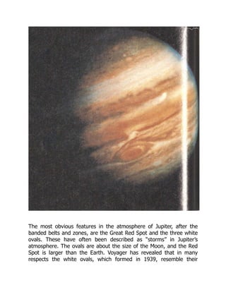
The most obviousfeatures in the atmosphere of Jupiter, after the
banded belts and zones, are the Great Red Spot and the three white
ovals. These have often been described as “storms” in Jupiter’s
atmosphere. The ovals are about the size of the Moon, and the Red
Spot is larger than the Earth. Voyager has revealed that in many
respects the white ovals, which formed in 1939, resemble their
61.
125
ancient red relative.All four spots are southern hemispheric
anticyclonic features that exhibit counterclockwise motion; hence
they are meteorologically similar. Other smaller bright elliptical and
circular spots also exhibit anticyclonic motion, rotating clockwise in
the northern hemisphere and counterclockwise in the southern
hemisphere. In general, these features are circled by filamentary
rings that are darker than the spots they surround. Hints of interior
spiral structure can be seen in some of these spots. All the elliptical
features in the southern hemisphere lie to the south of the strong
westward-blowing jet streams. The spots tend to become rounder the
closer they are to the poles.
Along the northern edge of the equator are a number of cloud
plumes, which appear to be regularly spaced all around the planet.
Some of the plumes have been observed to brighten rapidly, which
may be an indication of convective activity; indeed, some of the
plume structures seem to resemble the convective storms that form
in the Earth’s tropics. The plumes travel eastward at speeds ranging
from about 100 to 150 meters per second, but they do not move as a
unit.
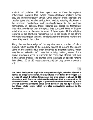
The Great Red Spot of Jupiter is a magnificent sight, whether viewed in
normal or exaggerated color. These pictures were taken by Voyager 1 at
a range of about 1 million kilometers; the area shown is about 25 000
kilometers, with features visible on the originals that are as small as 30
kilometers across. The Red Spot is partly obscured on the north by a thin
layer of overlying ammonia cirrus cloud. South of the Red Spot is one of
the three white ovals, which are also anticyclonic vortices in the
atmosphere.
126
The red andblue have been greatly exaggerated in this frame to bring
out fine detail in the cloud structure. [P-21431C]
The most visible cloud interactions take place in the region of
the Great Red Spot. Material within the Red Spot rotates
about once every six days. Infrared measurements show that the Red
Spot is a region of atmospheric upwelling, which extends to very high
altitudes; however, the divergent flow suggested by this upwelling
seems to be very small—one bright feature was observed to circle the
Red Spot for sixty days without appreciably changing its distance
from the spot’s center. During the Voyager 1 flyby, spots were seen to
move toward the Red Spot from the east, flow along its northern
border, then either flow on to the west past the Red Spot or into the
outer regions of its vortex. A spot caught on the outer edge of the
Red Spot flow might break in two as it reached the eastern edge of
the spot, with one piece remaining in the vortex and the other
moving off to the east. Alternatively, a spot floating toward the Red
64.
Welcome to ourwebsite – the perfect destination for book lovers and
knowledge seekers. We believe that every book holds a new world,
offering opportunities for learning, discovery, and personal growth.
That’s why we are dedicated to bringing you a diverse collection of
books, ranging from classic literature and specialized publications to
self-development guides and children's books.
More than just a book-buying platform, we strive to be a bridge
connecting you with timeless cultural and intellectual values. With an
elegant, user-friendly interface and a smart search system, you can
quickly find the books that best suit your interests. Additionally,
our special promotions and home delivery services help you save time
and fully enjoy the joy of reading.
Join us on a journey of knowledge exploration, passion nurturing, and
personal growth every day!
testbankdeal.com


![Chapter 07 - Cash Flow Analysis
7-15
Copyright © 2014 McGraw-Hill Education. All rights reserved. No reproduction or distribution without the prior written consent of McGraw-Hill
Education.
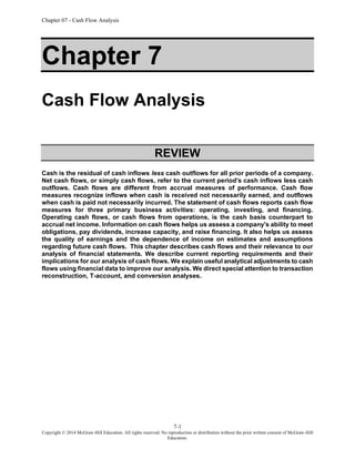
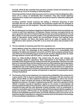
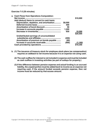
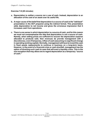
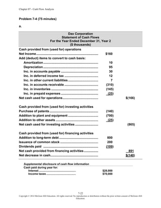
Exercise 7-9 (60 minutes)
a. Cash Collections Computation:
Accounts Receivable (Net)
Beg [a] 564.1
Sales [13] 6205.8 6145.4 Cash collections [b]
End [33] 624.5
Notes:
[a] Balance at 7/29/Year 10............................................ $624.5 [33]
Less: increase in Year 10......................................... (60.4) [61]
$564.1
[b]This amount is overstated by the provision for doubtful accounts expense that is included in
another expense category.
b. Cash Dividends Paid Computation:
Dividends Payable
Dividend paid [77] 137.5 32.3 Beg [43]
142.2 Dividend declared [a] [89]
37.0 End [43]
Note [a]: Item [89] represents dividends declared, not dividends paid (see also Item [77]).
c. Cost of Goods and Services Produced Computation:
Inventories
Beg [34] 819.8
Amount to balance 3982.4
4095.5 Cost of products sold [14]
End [34] 706.7
d. The entry for the income tax provision for Year 11 is:
Income tax expense [27] ...................................... 265.9
Deferred income tax (current) plug.................. 12.1
Income tax payable............................................. 230.4
Deferred income tax (noncurrent) [a] ............... 23.4
Notes:
(1) The entry increases current liabilities by $12.1 since deferred income tax (current) is credited
by this amount. It also increases current liabilities by $230.4 [124A], the amount of income taxes
payable.
(2) The [a] is the difference in the balance of the noncurrent deferred income tax item [176] =
$258.5 - $235.1 = $23.4.
(3) Also, $23.4 + $12.1 = $35.5, which is total deferred tax [59] or [127A]](https://image.slidesharecdn.com/14601-250317025050-6c94ae1f/85/Financial-Statement-Analysis-11th-Edition-Subramanyam-Solutions-Manual-19-320.jpg)
![Chapter 07 - Cash Flow Analysis
7-16
Copyright © 2014 McGraw-Hill Education. All rights reserved. No reproduction or distribution without the prior written consent of McGraw-Hill
Education.
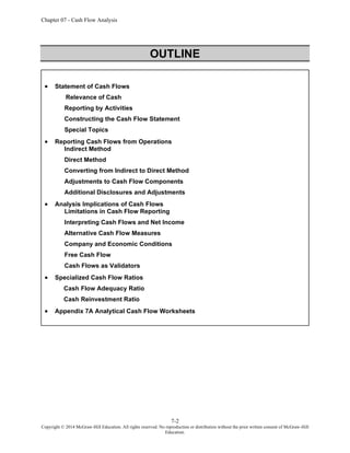
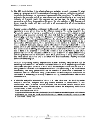
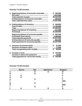
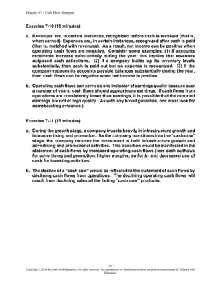
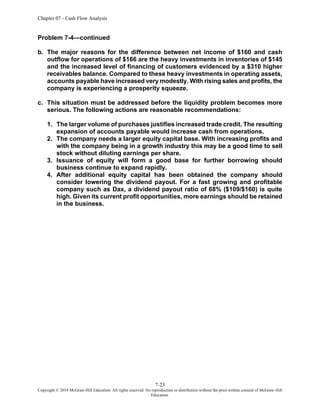
Exercise 7-9—continued
e. Depreciation expense has no effect on cash from operations. The credit, when
recording the depreciation expense, goes to accumulated depreciation, a
noncash account.
f. These provisions are added back because they affect only noncash accounts, the
charge to earnings must be removed in converting it to the cash basis.
g. The “Effect of exchange rate changes on cash” represents translation
adjustments (differences) arising from the translation of cash from foreign
currencies to the U.S. dollar.
h. Any gain or loss is reported under "other, net"—Item [60].
i. Free cash flows =
Cash flow from operations – Cash used for capital additions – Dividends paid
Year 11: $805.2 – $361.1 – $137.5 = $306.6
Year 10: $448.4 – $387.6 – $124.3 = $(63.5)
Year 9: $357.3 – $284.1 – $86.7 = $(13.5)
j. Start-up companies usually have greater capital addition requirements and lower
cash inflows from operations. Also, start-ups rarely pay cash dividends. Free
cash flow earned by start-up companies is usually used to fund the growth of the
company, especially if successful.
k. During the launch of a new product line, the statement of cash flows can be
affected in several ways. First, cash flow from operations is lower because
substantial advertising and promotion is required and sales growth has not yet
been maximized. Second, substantial capital additions are usually necessary to
provide the infrastructure for the new product line. Third, cash flow from
financing can be affected if financing is obtained to launch this new product line.](https://image.slidesharecdn.com/14601-250317025050-6c94ae1f/85/Financial-Statement-Analysis-11th-Edition-Subramanyam-Solutions-Manual-20-320.jpg)
![Chapter 07 - Cash Flow Analysis
7-18
Copyright © 2014 McGraw-Hill Education. All rights reserved. No reproduction or distribution without the prior written consent of McGraw-Hill
Education.
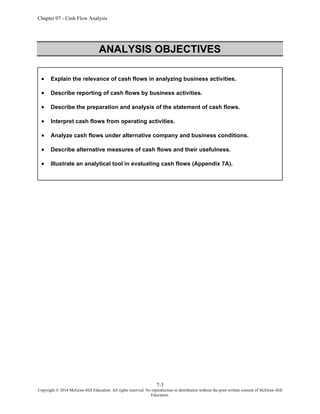
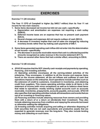
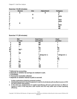
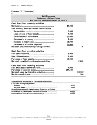
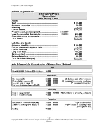
PROBLEMS
Problem 7-1 (60 minutes)
WORKSHEET TO COMPUTE CASH FLOW FROM OPERATIONS (IN MILLIONS)
DIRECT (INFLOW-OUTFLOW) PRESENTATION
CAMPBELL SOUP — YEAR ENDED JULY 28, YEAR 11
Ref. Reported Adjust. Revised
Cash Receipts from Operations
Net Sales ........................................................... 13 $6,204.1 $7.5 $6,211.6
Other revenue and income ............................. 19 26.0 C 26.0
(I) D in current receivables ............................. 61 17.1 C 17.1
(I) D in noncurrent receivables.......................
= CASH COLLECTIONS................................. $6,247.2 $7.5 $6,254.7
Cash Disbursements for Operations
Total expenses (include min. int. & taxes) a
$5,831.0 $7.5 $5,838.5
Less: Expenses & losses not using cash:
- Depreciation and amortization..................... 57 (208.6) (208.6)
- Noncurrent deferred income taxes.............. 59 (35.5) (35.5)
- Other, net........................................................ 60 (63.2) (63.2)
Change in Current Assets and Liabilities
related to Operations
I (D) in inventories ......................................... 62 $ (48.7) $ (48.7)
I (D) in prepaid expenses .............................. 35 (25.3) (25.3)
(I) D in accounts payable .............................. 41 42.8 42.8
(I) D in taxes payable ..................................... 44 (21.3) (21.3)
(I) D in accruals, payrolls, etc. b
................... 175 (26.8) (26.8)
I or D in noncurrent accounts c
.................... 5.8 0.0 5.8
= CASH DISBURSEMENTS ............................. $5,450.2 $7.5 $5,457.7
Dividends Received
Equity in income of
unconsolidated affiliates............................... 24 2.4 2.4
Distributions beyond equity
in income of affiliates c
.................................. 5.8 0.0 5.8
= Dividends from unconsol. affiliates ........... 169A $ 8.2 $0.0 $ 8.2
CASH FLOW FROM OPERATIONS ............... $ 805.2 $0.0 $ 805.2
a
Total costs and expenses [22A] + Taxes on earnings [27] + Minority interests [25] +
Interest income [19] = $5,531.9 + $265.9 + $7.2 + $26.0 = $5,831
b
It is assumed that accruals, payrolls, etc., are part of item [175].
c
A reconciling amount to tie in with the $8.2 dividends from affiliates (item 169A) versus
equity in earnings of affiliates (item 24).](https://image.slidesharecdn.com/14601-250317025050-6c94ae1f/85/Financial-Statement-Analysis-11th-Edition-Subramanyam-Solutions-Manual-22-320.jpg)
![Chapter 07 - Cash Flow Analysis
7-19
Copyright © 2014 McGraw-Hill Education. All rights reserved. No reproduction or distribution without the prior written consent of McGraw-Hill
Education.
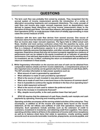
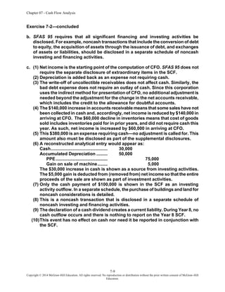
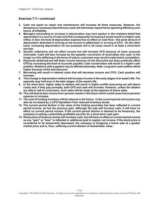
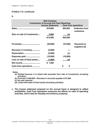
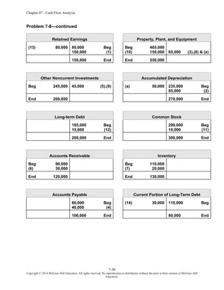
Problem 7-2 (75 minutes)
a.
WORKSHEET TO COMPUTE CASH FLOW FROM OPERATIONS (IN MILLIONS)
DIRECT (INFLOW-OUTFLOW) PRESENTATION
CAMPBELL SOUP YEAR ENDED JULY 29, YEAR 10
Ref. Reported Adjust. Revised
Cash Receipts from Operations
Net Sales ........................................................... 13 $6,205.8 $7.5 $6,213.3
Other revenue and income:
(I) D in current receivables ............................. 61 (60.4) (60.4)
(I) D in noncurrent receivables
Effect of translation adjustments ............... 0.0 0.0 0.0
= Cash Collections........................................... $6,145.4 $7.5 $6,152.9
Cash Disbursements for Operations
Total expenses (include interest &
taxes) [22A] + [27] + [25] ............................... $6,214.9 $7.5 $6,222.4
Less: Expenses & Losses not using cash
- Depreciation & amortization......................... 57 (200.9) (200.9)
- Noncurrent deferred income taxes.............. 59 (3.9) (3.9)
- Other provision for restructuring
and writedowns.............................................. 58 (339.1) (339.1)
- Other * ............................................................. 60 (24.7) (24.7)
- Other
Changes in Current Assets and Liabilities
related to operations
I (D) in inventories ......................................... 62 (10.7) (10.7)
I (D) in prepaid expense ................................
(I) D in accounts payable ..............................
(I) D in taxes payable .....................................
(I) D in accruals, payrolls, etc.......................
(I) D in dividends payable .............................
I or D other ** .................................................. 63 68.8 68.8
I or D in noncurrent amounts ....................... 0.0 0.0 0.0
= Cash Disbursements............................. $5,704.4 $7.5 $5,711.9
Dividends Received
Equity in income of unconsolidated
affiliates........................................................... 24 13.5 13.5
- Undistributed equity in income of
affiliates........................................................... 169A (6.1) 0.0 (6.1)
= Dividends from unconsol. affils.................. 7.4 7.4
Cash Flow From Operations........................... $ 448.4 $ 448.4
*
Other, net [60] $18.6 + [169A] $6.1 = $24.7
**
Campbell shows a combined figure instead of details of operating assets and liabilities.](https://image.slidesharecdn.com/14601-250317025050-6c94ae1f/85/Financial-Statement-Analysis-11th-Edition-Subramanyam-Solutions-Manual-23-320.jpg)
![Chapter 07 - Cash Flow Analysis
7-24
Copyright © 2014 McGraw-Hill Education. All rights reserved. No reproduction or distribution without the prior written consent of McGraw-Hill
Education.
Problem 7-5 (40 minutes)
Niagara Company
Statement of Cash Flows
For Year Ended December 31, Year 9
Cash flows from operating activities
Cash receipts from operations
Sales [a]................................................................... $980
Cash payments for operations
Purchases of inventory [b]..................................... (645)
Selling and general expenses ............................... (100)
Interest expense [c] ................................................ (40)
Income tax expense [d] .......................................... (30)
Cash flows from operations ........................................ $165
Cash flows from investing activities
Purchase of fixed assets........................................ (150)
Cash flows from financing activities
Repayment of notes payable ................................. (25)
Issuance of long-term debt .................................... 50
Cash dividends paid............................................... (30)
Cash flows used in financing...................................... (5)
Net increase in cash..................................................... $ 10
Beginning cash balance .............................................. 50
Ending cash balance.................................................... $ 60
Notes:
[a] Sales ................................................................................ $1,000
Less increase in receivables......................................... (20)
Cash collections ............................................................. $980
[b] Cost of goods sold ......................................................... $ (650)
Add increase in inventories........................................... (20)
Less increase in payables ............................................. 25
(645)
[c] Interest expense ............................................................. $ (50)
Less increase in interest payable ................................. 10
(40)
[d] Income tax expense ....................................................... $ (40)
Less increase in deferred income tax .......................... 10
(30)
Note: Purchase of fixed assets is computed from depreciation expense plus change in fixed
assets ($100+$50). Dividends paid is computed from net income and change in retained earnings
($60-$30).
Supporting schedule for CFO:
Net income ..................................................................................................... $ 60
Add depreciation ........................................................................................... 100
Increase in deferred tax ................................................................................ 10
Increase in receivables ................................................................................. (20)
Increase in inventory..................................................................................... (20)
Increase in accounts payable....................................................................... 25
Increase in interest payable ......................................................................... 10
Cash flows from operations ......................................................................... $165](https://image.slidesharecdn.com/14601-250317025050-6c94ae1f/85/Financial-Statement-Analysis-11th-Edition-Subramanyam-Solutions-Manual-28-320.jpg)
![Chapter 07 - Cash Flow Analysis
7-25
Copyright © 2014 McGraw-Hill Education. All rights reserved. No reproduction or distribution without the prior written consent of McGraw-Hill
Education.
Problem 7-6 (35 minutes)
Effects Analytical Entries (Optional)
a. [-Y, 11,000] Bad Debt Expense ........................ 11,000
[CC, 11,000] Allowance for Bad Debt ......... 11,000
b. [-Y, 16,000] Depreciation .................................. 16,000
[YA, 16,000] Accumulated Depreciation .... 16,000
c. [NAA, 100,000] Building ......................................... 100,000
[NDE, 100,000] Long-Term Note Payable ....... 100,000
d. None
e. None
f. [+C, 10,000] Cash............................................... 10,000
[-Y, 2,000] Loss ............................................... 2,000
[CC, 12,000] Inventory ................................. 12,000
g. [+C, 35,000] Cash............................................... 35,000
[DC, 5,000] Accounts Receivable.................... 5,000
[CC, 25,000] Inventory ................................. 25,000
[+Y, 15,000] Gain.......................................... 15,000
h. [CC, 3,000] Allowance...................................... 5,000
[-Y, 3,000] Bad Debt Expense ........................ 3,000
Accounts Receivable.............. 8,000
i. [AA, 100,000] Assets............................................ 100,000
[-C, 100,000] Cash......................................... 100,000
[-Y, 20,000] Depreciation expense................... 20,000
[YA, 20,000] Accumulated Depreciation .... 20,000
j. [+C, 8,000] Cash............................................... 8,000
[AD, 8,000] Loss on Sale.................................. 1,000
[YA, 1,000] Machinery (net) ....................... 9,000
[-Y, 1,000]](https://image.slidesharecdn.com/14601-250317025050-6c94ae1f/85/Financial-Statement-Analysis-11th-Edition-Subramanyam-Solutions-Manual-29-320.jpg)
![Chapter 07 - Cash Flow Analysis
7-26
Copyright © 2014 McGraw-Hill Education. All rights reserved. No reproduction or distribution without the prior written consent of McGraw-Hill
Education.
Problem 7-7 (60 minutes)
Part I.
Effects Analytical Entries (Optional)
a. [DL, 100,000] Current Portion of L-T Debt.......... 100,000
[-C, 100,000] Cash......................................... 100,000
b. [+C, 4,000] Cash............................................... 4,000
[AD, 4,000] Loss ............................................... 1,000
[YA, 1,000] Equipment ............................... 5,000
[-Y, 1,000]
c. [-Y, 75,000] Loss ............................................... 75,000
[CC, 75,000] Inventory ................................. 75,000
d. [+C, 28,000] Cash............................................... 28,000
[DE, 28,000] Paid-In Capital............................... 2,000
Treasury stock ........................ 30,000
e. [NAA, 300,000] Plant Assets .................................. 300,000
[NDE, 300,000] Mortgage Payable................... 250,000
Mortgage Payable—Current... 50,000
f. [+C, 6,000] Investment..................................... 30,000
[+Y, 30,000] Equity in NI of Subsidiary ...... 30,000
[YS, 24,000] Cash............................................... 6,000
Investment 6,000
g. [+C, 10,000] Cash............................................... 10,000
[+Y, 40,000] Accounts Receivable, current...... 10,000
[DC, 10,000] Accounts Receivable, noncurrent 20,000
[NC, 20,000] Sales ........................................ 40,000
h. [DC, 9,000] Inventory........................................ 9,000
[+Y, 9,000] Cost of Goods Sold ................ 9,000
i. [DC, 260,000] Current Assets .............................. 260,000
[CC, 160,000] Plant and Equipment .................... 670,000
[DE, 410,000] Current Liabilities. .................. 160,000
[-C, 360,000] Long-Term Debt...................... 410,000
Cash ($400-$40) ...................... 360,000
j. [-Y, 60,000] Expense......................................... 60,000
[CC, 60,000] Allowance for doubtful accounts 60,000](https://image.slidesharecdn.com/14601-250317025050-6c94ae1f/85/Financial-Statement-Analysis-11th-Edition-Subramanyam-Solutions-Manual-30-320.jpg)
![Chapter 07 - Cash Flow Analysis
7-27
Copyright © 2014 McGraw-Hill Education. All rights reserved. No reproduction or distribution without the prior written consent of McGraw-Hill
Education.
Problem 7-7—continued
Part II.
Effects Analytical Entries (Optional)
a. [AA, 120,000] Investment..................................... 120,000
[-C, 120,000] Cash......................................... 120,000
b. [YS, 7,500] Investment..................................... 7,500
[+Y, 7,500] Equity in Earnings .................. 7,500
c. [+C, 3,000] Investment..................................... 9,000
[+Y, 9,000] Equity in Earnings…………….. 9,000
[YS, 6,000] Cash............................................... 3,000
Investment............................... 3,000
d. [+C, 4,000] Cash............................................... 4,000
[AD, 4,000] Equipment (net) ...................... 3,000
[YS, 1,000] Gain on Sale ........................... 1,000
[+Y, 1,000]
e. [+C, 60,000] Cash............................................... 60,000
[IL, 60,000] Note Payable (current) ........... 60,000
f. [NDR, 9,000] Bonds Payable .............................. 9,000
[NDE, 9,000] Common stock........................ 2,000
Paid-In Capital......................... 7,000
g. [+C, 6,000] Cash............................................... 6,000
[DE, 6,000] Treasury stock ........................ 4,000
Paid-In Capital......................... 2,000
h1.[AA, 200,000] Investment..................................... 200,000
[DE, 100,000] Common stock........................ 100,000
[-C, 100,000] Cash......................................... 100,000
h2.[DC, 80,000] Current Assets ($120-$40)............ 80,000
[AA, 180,000] Plant and Equipment .................... 180,000
[DE, 140,000] Current Liabilities ................... 60,000
[-C, 60,000] Long-Term Debt...................... 40,000
Common stock........................ 100,000
Cash ($100-$40) ...................... 60,000
i. [-Y, 4,000] Minority Interest Expense ............ 4,000
[YA, 4,000] Minority Interest...................... 4,000](https://image.slidesharecdn.com/14601-250317025050-6c94ae1f/85/Financial-Statement-Analysis-11th-Edition-Subramanyam-Solutions-Manual-31-320.jpg)
![Chapter 07 - Cash Flow Analysis
7-28
Copyright © 2014 McGraw-Hill Education. All rights reserved. No reproduction or distribution without the prior written consent of McGraw-Hill
Education.
Problem 7-7—continued
Part II.
Effects Analytical Entries (Optional)
j. [-Y, 50,000] Inventory Loss .............................. 50,000
[CC, 50,000] Inventory ................................. 50,000
k. None Allow. for doubtful accounts........ 1,200
Accounts receivable 1,200
l. [NAA, 120,000] Leased Equipment........................ 120,000
[NDE, 120,000] Long-Term debt ...................... 120,000
m. None Retained Earnings ........................ 180,000
Common stock ....................... 120,000
Paid-in Capital......................... 60,000
n. [-Y, 27,000] Bad Debts Expense ...................... 27,000
[CC, 27,000] Allow for Doubtful Accounts . 27,000](https://image.slidesharecdn.com/14601-250317025050-6c94ae1f/85/Financial-Statement-Analysis-11th-Edition-Subramanyam-Solutions-Manual-32-320.jpg)

![112
[that both the light and dark markings are of planetary scale]
suggests that they must be related.”
Ed Stone speculated about the other two Galilean satellites.
Ganymede and Callisto are essentially identical in size, mass, and
probably composition. By examining them, we can perhaps learn
what happens when bodies with very similar chemistry have different
“life histories” and different surface properties (there are indications
that Ganymede’s crust may not have been as rigid as Callisto’s).
Going further, he added that Callisto and Mercury, the least dense
and the most dense, respectively, of the terrestrial-style planets,
although totally different in composition and density, seem to have
similar surfaces and similar histories. What would have happened to
Mercury if it had been made of ice, water, and rock as Callisto is?
Would it have evolved as Callisto did?
One of the most spectacular of the Voyager 2 images was obtained from
inside the shadow of Jupiter. Looking back toward the planet and the
rings with its wide-angle camera, the spacecraft took these photos on
July 10 from a distance of 1.5 million kilometers. The ribbon-like nature
of the rings is clearly shown. The planet is outlined by sunlight scattered](https://image.slidesharecdn.com/14601-250317025050-6c94ae1f/85/Financial-Statement-Analysis-11th-Edition-Subramanyam-Solutions-Manual-36-320.jpg)
![from a haze layer high in the atmosphere. On each side, the arms of the
ring curving back toward the spacecraft are cut off by the planet’s
shadow as they approach the brightly outlined disk. [P-21774B/W]
The rings of Jupiter proved to be unexpectedly bright when seen with the
Sun nearly behind them. Strong forward scattering of sunlight is
characteristic of small particles. These two views were obtained by
Voyager 2 on July 10 from a perspective inside the shadow of Jupiter.
The distance of the spacecraft from the rings was about 1.5 million
kilometers. Although the resolution has been degraded by camera motion
during the time exposures, these images reveal that the rings have some
radial structure. [260-610B/W and 260-674]](https://image.slidesharecdn.com/14601-250317025050-6c94ae1f/85/Financial-Statement-Analysis-11th-Edition-Subramanyam-Solutions-Manual-37-320.jpg)
![HIGHLIGHTS OF THE VOYAGER 2 SCIENTIFIC FINDINGS
[3]
Atmosphere
The main atmospheric jet streams were present during both
Voyager encounters, with some changes in velocity.](https://image.slidesharecdn.com/14601-250317025050-6c94ae1f/85/Financial-Statement-Analysis-11th-Edition-Subramanyam-Solutions-Manual-38-320.jpg)
![114
The abundance of oxygen and sulfur relative to helium at high
energy increases with decreasing distance from Jupiter.
Measurements of high energy oxygen suggest that these nuclei
are diffusing inward toward Jupiter.
The ultraviolet emission from the Io plasma torus was twice as
bright as four months earlier and the temperature had
decreased by 30 percent to 60 000 K.
The low-frequency (kilometric) radio emissions from Jupiter
have a strong latitude dependence and often contain
narrowband emissions that drift to lower or higher frequencies
with time.
A complex magnetospheric interaction with Ganymede was
observed in the magnetic field, plasma, and energetic particles
up to about 200 000 kilometers from the satellite.
[3]
Adapted from a summary prepared by E. C. Stone and A. L.
Lane for the Voyager 2 Thirty-Day Report.
A new inner satellite of Jupiter, provisionally designated 1979J1, was
discovered by David Jewitt and Ed Danielson of Caltech in these Voyager
2 ring photographs.](https://image.slidesharecdn.com/14601-250317025050-6c94ae1f/85/Financial-Statement-Analysis-11th-Edition-Subramanyam-Solutions-Manual-41-320.jpg)
![In a 15-second exposure with the wide-angle camera, the edge-on ring
shows as a faint line, and the satellite is the dot indicated by the arrow.
[260-807]
In a narrow angle 96-second exposure, the motion of the satellite can be
seen. Again, the faint band is the ring, blurred by camera motion, and the
arrow indicates the streak due to the satellite. A star streak is located
above and to the left of the satellite; note that the length and angle of
the two trails are different, owing to satellite motion. [P-22172]](https://image.slidesharecdn.com/14601-250317025050-6c94ae1f/85/Financial-Statement-Analysis-11th-Edition-Subramanyam-Solutions-Manual-42-320.jpg)
![116
designated 1979J2. This satellite orbits between Io and Amalthea with a
period of 16 hours and 11 minutes. [P-22580B/W]](https://image.slidesharecdn.com/14601-250317025050-6c94ae1f/85/Financial-Statement-Analysis-11th-Edition-Subramanyam-Solutions-Manual-45-320.jpg)
![117
The Jupiter seen by the Voyager cameras is a cloud-belted world of rapid
jet streams and complex cloud forms. Prominent in this Voyager 1 image,
taken February 5 at a range of 28.4 million kilometers, is the alternating
structure of light zones and dark belts, and the Great Red Spot and
numerous smaller spots. Also easily visible are the two inner Galilean
satellites, Io and Europa. The resolution in this picture is 500 kilometers,
about five times better than can be obtained from Earth-based
telescopes. Callisto can be faintly seen at the lower left. [P-21083C]](https://image.slidesharecdn.com/14601-250317025050-6c94ae1f/85/Financial-Statement-Analysis-11th-Edition-Subramanyam-Solutions-Manual-46-320.jpg)
![119
hydrocarbon “smog”; ammonia; ammonium hydrosulfide; water-ice, and
liquid water. [260-828]
Cloud top-aerosols
Ammonia crystals
Ammonium hydrosulfide clouds
Ice crystal clouds
Water droplets
Trace compounds
Fluid molecular hydrogen
Transition Zone
Fluid metallic hydrogen
Possible core
The primary constituents of Jupiter have long been suspected
to be hydrogen and helium, the two simplest and lightest
atoms. However, it has proved impossible to derive accurate
measurements of the abundance of these two elements from
astronomical observations. On the basis of a rather simple infrared
measurement, Pioneer investigators found He/H₂ = 0.14 ± 0.08. On
Voyager, IRIS was able to obtain much improved infrared spectra,
yielding an initial value of He/H₂ = 0.11 ± 0.3. Voyager scientists
expect that further analysis will reduce the uncertainty to about ±
0.01. The ratio of 0.11 is in excellent agreement with the solar value
of about 0.12, supporting the idea that Jupiter and the Sun have
similar elemental compositions.
Astronomers have known for a long time that, in addition to
hydrogen and helium, the compounds methane (CH₄) and ammonia
(NH₃) are present in the visible atmosphere of Jupiter. In the 1970s,
additional spectra in the infrared resulted in the discovery of water
(H₂O), ethane (C₂H₆), germane (GeH₄), acetylene (C₂H₂), phosphine
(PH₃), carbon monoxide (CO), hydrogen cyanide (HCN), and carbon
dioxide (CO₂). All these are trace constituents, with two of them,
ethane and acetylene, apparently formed at high altitudes by the
action of sunlight on methane.](https://image.slidesharecdn.com/14601-250317025050-6c94ae1f/85/Financial-Statement-Analysis-11th-Edition-Subramanyam-Solutions-Manual-50-320.jpg)
![degrees apart in longitude, but a fourth oval at the other quadrant is
missing. The irregular black areas at each pole are places for which no
Voyager data exist. The resolution of the original pictures from which
these polar projections were made was about 600 kilometers.
North pole. [P-21638C]](https://image.slidesharecdn.com/14601-250317025050-6c94ae1f/85/Financial-Statement-Analysis-11th-Edition-Subramanyam-Solutions-Manual-53-320.jpg)
![121
122
South pole. [P-21639C]
Various forms of elemental sulfur might be responsible for the
riot of color we see on Jupiter. Sulfur forms polymers (S₃, S₄,
S₅, S₈,) that are yellow, red, and brown, but no sulfur in any form
has been detected on Jupiter. “We never promised you we were](https://image.slidesharecdn.com/14601-250317025050-6c94ae1f/85/Financial-Statement-Analysis-11th-Edition-Subramanyam-Solutions-Manual-54-320.jpg)
![going to identify the colors on Jupiter with this mission,” one of the
atmospheric scientists remarked, “but we will have a probe that is
going into the atmosphere in the mid-1980s—Galileo.” Perhaps the
mystery of the Jovian clouds will have to wait till then.
Temperature maps of Jupiter were obtained by IRIS in radiation
arising at different levels above the clouds. Maps show temperatures
at pressures of 0.8 atmosphere near the clouds, and 0.2 atmosphere
near the top of the troposphere. In addition to the low temperatures
over the bright zones and the higher temperatures over dark belts,
there is a great deal of smaller scale structure. It is interesting that a
cold area corresponding to the Great Red Spot is clearly visible even
near the top of the troposphere, indicating that this feature disturbs
the atmosphere to very high altitudes.
The structure of the atmosphere of Jupiter above the troposphere
was investigated through the radio occultation experiment as well as
by IRIS. The level in which the minimum temperature of about -173°
C occurs has a pressure of 0.1 atmosphere. Above this point lies the
stratosphere, in which temperatures increase with altitude as a result
of sunlight absorbed by the gas or by aerosol particles resembling
smog. At 70 kilometers above the ammonia clouds, the temperature
is about -113° C. Above this level, the temperature stays
approximately constant, although at extreme altitudes the
temperature again rises in the ionosphere.
If one could “unwrap” Jupiter like a map, views such as these would be
obtained. The comparison between the pictures shows the relative
motions of features in Jupiter’s atmosphere. It can be seen, for example,
that the Great Red Spot moved westward and the white ovals eastward
during the time between the acquisition of these pictures. Regular plume
patterns are equidistant around the northern edge of the equator, while a
train of small spots moved eastward at approximately latitude 80° S. In
addition to these relative motions, significant changes are evident in the
recirculating flow east of the Great Red Spot, in the disturbed region
west of the Great Red Spot, and as seen in the brightening of material
spreading into the equatorial region from the more southerly latitudes.
[P-21771C]](https://image.slidesharecdn.com/14601-250317025050-6c94ae1f/85/Financial-Statement-Analysis-11th-Edition-Subramanyam-Solutions-Manual-55-320.jpg)
![Differing characteristics of Jupiter’s meteorology are apparent in high-
resolution images, such as this one taken by Voyager 1 on March 2 at a
range of 4 million kilometers. The well-defined pale orange line running
from southwest to northeast (north is at the top) marks the high-speed
north temperate current with wind speeds of about 120 meters per
second. Toward the top of the picture, a weaker jet of approximately 30
meters per second is characterized by wave patterns and cloud features
which have been observed to rotate in a clockwise manner at these
latitudes of about 35°N. These clouds have been observed to have
lifetimes of one to two years. [P-21193C]
On a broader time scale, greater changes on the face of Jupiter can
be seen. Features drift around the planet; even the large white ovals
and the Great Red Spot slide along in their respective latitudes. Belts](https://image.slidesharecdn.com/14601-250317025050-6c94ae1f/85/Financial-Statement-Analysis-11th-Edition-Subramanyam-Solutions-Manual-57-320.jpg)
![Jupiter’s cloud patterns changed significantly in the few months between
the two Voyager flybys. Most of the changes are the result of differential
rotation, in which the prevailing winds at different latitudes shift long-
lived features with respect to those north or south. Thus, for example,
the three large white ovals shifted nearly 90 degrees in longitude,
relative to the Great Red Spot, between March and July. [P-21599]](https://image.slidesharecdn.com/14601-250317025050-6c94ae1f/85/Financial-Statement-Analysis-11th-Edition-Subramanyam-Solutions-Manual-59-320.jpg)
![This frame is in natural color. [P-21430C]](https://image.slidesharecdn.com/14601-250317025050-6c94ae1f/85/Financial-Statement-Analysis-11th-Edition-Subramanyam-Solutions-Manual-62-320.jpg)
![126
The red and blue have been greatly exaggerated in this frame to bring
out fine detail in the cloud structure. [P-21431C]
The most visible cloud interactions take place in the region of
the Great Red Spot. Material within the Red Spot rotates
about once every six days. Infrared measurements show that the Red
Spot is a region of atmospheric upwelling, which extends to very high
altitudes; however, the divergent flow suggested by this upwelling
seems to be very small—one bright feature was observed to circle the
Red Spot for sixty days without appreciably changing its distance
from the spot’s center. During the Voyager 1 flyby, spots were seen to
move toward the Red Spot from the east, flow along its northern
border, then either flow on to the west past the Red Spot or into the
outer regions of its vortex. A spot caught on the outer edge of the
Red Spot flow might break in two as it reached the eastern edge of
the spot, with one piece remaining in the vortex and the other
moving off to the east. Alternatively, a spot floating toward the Red](https://image.slidesharecdn.com/14601-250317025050-6c94ae1f/85/Financial-Statement-Analysis-11th-Edition-Subramanyam-Solutions-Manual-63-320.jpg)