Downloaded 30 times

![PPCM formulation for 2D transient flow equation for
confined aquifer
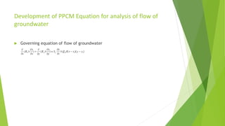
The transient of groundwater in homogeneous isotropic media in 2D can be written as
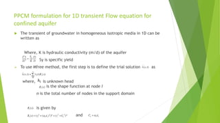
Again to use Mfree method, the first step is to define the trial solution as
where,
Single and double derivatives of shape function w.r.t x and y can be written as
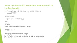
Putting these equation in first equation and arranging the terms, we get
where, [K1] is global matrix of shape function
[K2] is global matrix of double derivative of shape function w.r.t. x
[K3] is global matrix of double derivative of shape function w.r.t y](https://image.slidesharecdn.com/finalbtppresentation-141113051845-conversion-gate01/85/Meshless-Point-collocation-Method-For-1D-and-2D-Groundwater-Flow-Simulation-8-320.jpg)
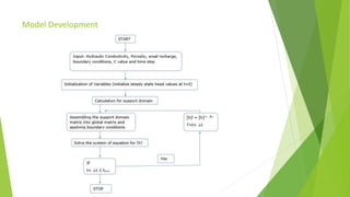
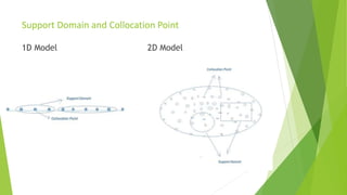

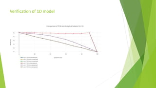
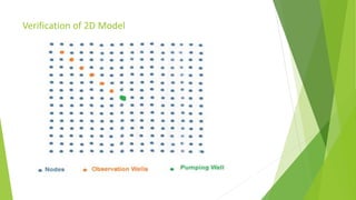
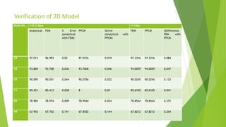
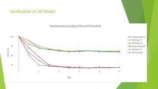
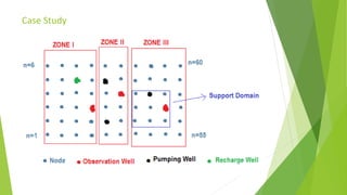


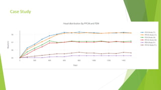


This document describes the development of a meshless point collocation method (PPCM) for simulating 1D and 2D groundwater flow. PPCM is a numerical technique that can establish algebraic equations over a problem domain without a predefined mesh, using scattered nodes. The document outlines the governing equations for 1D and 2D transient groundwater flow. It then describes how PPCM formulates these equations by defining a trial solution using shape functions and radial basis functions. The document verifies the 1D and 2D PPCM models against analytical and finite element method solutions. It also presents a case study application of the 2D PPCM model to a hypothetical confined aquifer with varying properties.