Fast Distributed Online Classification
Ram Sriharsha (Product Manager, Apache Spark, Databricks)
Prasad Chalasani (SVP Data Science, MediaMath)
13 April, 2016
Summary
We leveraged recent machine-learning research to develop a
I fast, practical,
I scalable (up to 100s of Millions of sparse features)
I online,
I distributed (built on Apache Spark),
I single-pass,
ML classifier that has significant advantages
over most similar ML packages.
Key Conceptual Take-aways
I Supervised Machine Learning
I Online vs Batch Learning, and importance of Online
I Challenges in online-learning
I Distributed implementation in Spark.
Supervised Machine Learning: Overview
Given:
I labeled training data,
Goal:
I fit a model to predict labels on (unseen) test data.
Supervised Machine Learning: Overview
Given:
I training data D: n labeled examples
{(x1, y1), (x2, y2), . . . , (xn, yn)} where
I xi is a k-dimensional feature-vector
I yi is the label (0 or 1) that we want to predict.
I an error (or loss) metric L(p, y) from predicting p when true
label is y.
Supervised Machine Learning: Overview
Given:
I training data D: n labeled examples
{(x1, y1), (x2, y2), . . . , (xn, yn)} where
I xi is a k-dimensional feature-vector
I yi is the label (0 or 1) that we want to predict.
I an error (or loss) metric L(p, y) from predicting p when true
label is y.
Fix a family of functions fw (x) œ F that are parametrised by a
weight-vector w.
Goal: find w that minimizes average loss over D:
L(w) =
1
n
nÿ
i=1
Li (w) =
1
n
nÿ
i=1
L(fw (xi ), yi ).
Logistic Regression
Logistic model fw (x) = 1
1+e≠w·x
Probability interpretation
Logistic Regression
Logistic model fw (x) = 1
1+e≠w·x
Probability interpretation
Loss Function Li (w) = ≠yi ln(fw (xi )) ≠ (1 ≠ yi ) ln(1 ≠ fw (xi ))
Logistic Regression
Logistic model fw (x) = 1
1+e≠w·x
Probability interpretation
Loss Function Li (w) = ≠yi ln(fw (xi )) ≠ (1 ≠ yi ) ln(1 ≠ fw (xi ))
Overall Loss L(w) =
qn
i=1 Li (w)
Logistic Regression
Logistic model fw (x) = 1
1+e≠w·x
Probability interpretation
Loss Function Li (w) = ≠yi ln(fw (xi )) ≠ (1 ≠ yi ) ln(1 ≠ fw (xi ))
Overall Loss L(w) =
qn
i=1 Li (w)
L(w) is convex:
I no local minima
I di erentiate and follow gradients
Logistic Regression: gradient descent
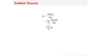
Gradient Descent
Basic idea:
I start with an initial guess of weight-vector w
I at iteration t, update w to a new weight-vector wÕ:
wÕ
= w ≠ ⁄gt
where
I gt is the (vector) gradient of L(w) w.r.t. w at time t,
I ⁄ is the learning rate.
Gradient Descent
Gradient gt =∆ step direction
Learning rate ⁄ =∆ step size
Gradient Descent
gt =
ˆL(w)
ˆw
=
ÿ
i
ˆLi (w)
ˆw
=
ÿ
i
gti
Gradient Descent
gt =
ˆL(w)
ˆw
=
ÿ
i
ˆLi (w)
ˆw
=
ÿ
i
gti
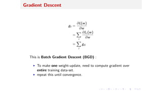
This is Batch Gradient Descent (BGD) :
I To make one weight-update, need to compute gradient over
entire training data-set.
I repeat this until convergence.
Gradient Descent
gt =
ˆL(w)
ˆw
=
ÿ
i
ˆLi (w)
ˆw
=
ÿ
i
gti
This is Batch Gradient Descent (BGD) :
I To make one weight-update, need to compute gradient over
entire training data-set.
I repeat this until convergence.
BGD is not scalable to large data-sets.
Online (Stochastic) Gradient Descent (SGD)
A drastic simplification:
Instead of computing gradient based on entire training data-set
gt =
ÿ
i
ˆLi (w)
ˆw
,
and doing an update wÕ = w ≠ ⁄gt.
Online (Stochastic) Gradient Descent (SGD)
A drastic simplification: Shu e data-set (if not naturally shu ed),
Compute gradient based on a one example
gti =
ˆLi (w)
ˆw
,
and do an update wÕ = w ≠ ⁄gti .
Batch vs Online Gradient Descent
Batch:
I to make one step, compute gradient w.r.t. entire data-set
I extremely slow updates
I correct gradient
Batch vs Online Gradient Descent
Batch:
I to make one step, compute gradient w.r.t. entire data-set
I extremely slow updates
I correct gradient
Online:
I to make one step, compute gradient w.r.t. one example:
I extremely fast updates
I not necessarily correct gradient
Visualize Batch vs Stochastic Gradient Descent
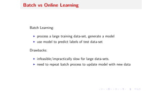
Batch vs Online Learning
Batch Learning:
I process a large training data-set, generate a model
I use model to predict labels of test data-set
Batch vs Online Learning
Batch Learning:
I process a large training data-set, generate a model
I use model to predict labels of test data-set
Drawbacks:
I infeasible/impractically slow for large data-sets.
I need to repeat batch process to update model with new data
Batch vs Online Learning
Online Learning:
I for each “training” example:
Batch vs Online Learning
Online Learning:
I for each “training” example:
I generate prediction (score),
Batch vs Online Learning
Online Learning:
I for each “training” example:
I generate prediction (score),
I compare with true label,
Batch vs Online Learning
Online Learning:
I for each “training” example:
I generate prediction (score),
I compare with true label,
I update model (weights w)
Batch vs Online Learning
Online Learning:
I for each “training” example:
I generate prediction (score),
I compare with true label,
I update model (weights w)
I for each “test” example:
Batch vs Online Learning
Online Learning:
I for each “training” example:
I generate prediction (score),
I compare with true label,
I update model (weights w)
I for each “test” example:
I predict with latest learned model (weights w)
Batch vs Online Learning
Online Learning benefits:
I does not pre-process enire training data-set
Batch vs Online Learning
Online Learning benefits:
I does not pre-process enire training data-set
I does not explicitly retain previously-seen examples
Batch vs Online Learning
Online Learning benefits:
I does not pre-process enire training data-set
I does not explicitly retain previously-seen examples
I extremely light-weight: space and time-e cient
Batch vs Online Learning
Online Learning benefits:
I does not pre-process enire training data-set
I does not explicitly retain previously-seen examples
I extremely light-weight: space and time-e cient
I no distinct “training” and “testing” phases:
Batch vs Online Learning
Online Learning benefits:
I does not pre-process enire training data-set
I does not explicitly retain previously-seen examples
I extremely light-weight: space and time-e cient
I no distinct “training” and “testing” phases:
I incremental, continual learning
Batch vs Online Learning
Online Learning benefits:
I does not pre-process enire training data-set
I does not explicitly retain previously-seen examples
I extremely light-weight: space and time-e cient
I no distinct “training” and “testing” phases:
I incremental, continual learning
I adapts to changing patterns
I easily update existing model with new data
I better generalization to unseen observations.
The Online Learning Paradigm
As each labeled example (xi , yi ) is seen,
I make prediction given only current weight-vector w
I update weight-vector w
Online Learning: Use Scenarios
I extremely large data-sets where
Online Learning: Use Scenarios
I extremely large data-sets where
I batch learning is computationally infeasible/impractical, and
Online Learning: Use Scenarios
I extremely large data-sets where
I batch learning is computationally infeasible/impractical, and
I it’s possible to only do a single pass over the data.
Online Learning: Use Scenarios
I extremely large data-sets where
I batch learning is computationally infeasible/impractical, and
I it’s possible to only do a single pass over the data.
I data arrives in real-time, and
Online Learning: Use Scenarios
I extremely large data-sets where
I batch learning is computationally infeasible/impractical, and
I it’s possible to only do a single pass over the data.
I data arrives in real-time, and
I decisions/predictions must be made quickly
Online Learning: Use Scenarios
I extremely large data-sets where
I batch learning is computationally infeasible/impractical, and
I it’s possible to only do a single pass over the data.
I data arrives in real-time, and
I decisions/predictions must be made quickly
I learned model needs to adapt quickly to recent observations.
Online Learning Examples
Online Learning Example: Advertising (MediaMath)
Listen to 100 billion ad-opportunities daily from Ad Exchanges.
Online Learning Example: Advertising (MediaMath)
Listen to 100 billion ad-opportunities daily from Ad Exchanges.
For each opportunity, need to predict whether exposed user will buy,
as function of several features:
I hour_of_day, browser_type, geo_region, age, . . .
Online Learning Example: Advertising (MediaMath)
Listen to 100 billion ad-opportunities daily from Ad Exchanges.
For each opportunity, need to predict whether exposed user will buy,
as function of several features:
I hour_of_day, browser_type, geo_region, age, . . .
Online learning benefits:
I fast update of learned model to reflect latest observations
I light-weight models extremely quick to compute
Online Learning: IOT
Vast amounts of data; need to adapt, respond quickly.
Online Learning: IOT
Vast amounts of data; need to adapt, respond quickly.
Nest Thermostats: behavior data =∆ predict preferred room temp.
Online Learning: IOT
Vast amounts of data; need to adapt, respond quickly.
Nest Thermostats: behavior data =∆ predict preferred room temp.
Self-driving Cars: (sensor data, other cars) =∆ predict collision
Online Learning: IOT
Vast amounts of data; need to adapt, respond quickly.
Nest Thermostats: behavior data =∆ predict preferred room temp.
Self-driving Cars: (sensor data, other cars) =∆ predict collision
Clinical: Sensors (activity, vitals, . . . ) =∆ predict cardiac event
Online Learning: IOT
Vast amounts of data; need to adapt, respond quickly.
Nest Thermostats: behavior data =∆ predict preferred room temp.
Self-driving Cars: (sensor data, other cars) =∆ predict collision
Clinical: Sensors (activity, vitals, . . . ) =∆ predict cardiac event
Smart cities: tra c sensors =∆ predict congestion
Online Learning: Challenge #1
Feature scale di erences
Online Learning: Feature Scaling
Example from wearable devices domain:
I feature 1 = heart-rate, range 40 to 200
I feature 2 = step-count, range 0 to 500,000
Online Learning: Feature Scaling
Example from wearable devices domain:
I feature 1 = heart-rate, range 40 to 200
I feature 2 = step-count, range 0 to 500,000
Extreme scale di erences =∆ convergence problems.
Convergence much faster when features are of same scale:
I normalize each feature by dividing by its max possible value.
Online Learning: Feature Scaling
But often:
I range of features not known in advance, and
I we cannot make a separate pass over the data to find ranges.
Online Learning: Feature Scaling
But often:
I range of features not known in advance, and
I we cannot make a separate pass over the data to find ranges.
=∆ Need single-pass algorithms that
adaptively normalize features with each new observation.
[Ross,Mineiro,Langford 2013] proposed such an algorithm,
which we implemented in our online ML system.
Online Learning Challenge #2:
(Sparse) Feature frequency di erences
Online Learning: Feature Frequency Di erences
Some sparse features occur much more frequently than others, e.g.:
I categorical feature country with 200 values,
Online Learning: Feature Frequency Di erences
Some sparse features occur much more frequently than others, e.g.:
I categorical feature country with 200 values,
I encoded as a vector of length 200 with exactly one entry = 1,
and the rest 0
Online Learning: Feature Frequency Di erences
Some sparse features occur much more frequently than others, e.g.:
I categorical feature country with 200 values,
I encoded as a vector of length 200 with exactly one entry = 1,
and the rest 0
I country=USA may occur much more often than
country=Belgium
Online Learning: Feature Frequency Di erences
Some sparse features occur much more frequently than others, e.g.:
I categorical feature country with 200 values,
I encoded as a vector of length 200 with exactly one entry = 1,
and the rest 0
I country=USA may occur much more often than
country=Belgium
I indicator feature visited_site = 1 much more often than
purchased=1.
Online Learning: Feature Frequency Di erences
Often, rare features much more predictive than frequent features.
Same learning rate for all features =∆ slow convergence.
Online Learning: Feature Frequency Di erences
Often, rare features much more predictive than frequent features.
Same learning rate for all features =∆ slow convergence.
=∆ rare features should have larger learning rates:
I bigger steps whenever a rare feature is seen
I much faster convergence
Online Learning: Feature Frequency Di erences
Often, rare features much more predictive than frequent features.
Same learning rate for all features =∆ slow convergence.
=∆ rare features should have larger learning rates:
I bigger steps whenever a rare feature is seen
I much faster convergence
E ectively, the algo pays more attention to rare features
Enables finding rare but predictive features.
Online Learning: Feature Frequency Di erences
Often, rare features much more predictive than frequent features.
Same learning rate for all features =∆ slow convergence.
=∆ rare features should have larger learning rates:
I bigger steps whenever a rare feature is seen
I much faster convergence
E ectively, the algo pays more attention to rare features
Enables finding rare but predictive features.
ADAGRAD is an algorithm for this [Duchi,Hazan,Singer 2010], and
we implemented this in our learning system.
Online Learning Challenge #3:
Encoding sparse features
Online Learning: Sparse Features
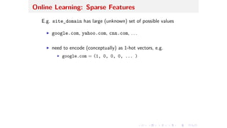
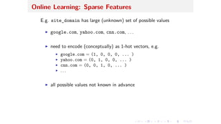
E.g. site_domain has large (unknown) set of possible values
I google.com, yahoo.com, cnn.com, . . .
Online Learning: Sparse Features
E.g. site_domain has large (unknown) set of possible values
I google.com, yahoo.com, cnn.com, . . .
I need to encode (conceptually) as 1-hot vectors, e.g.
Online Learning: Sparse Features
E.g. site_domain has large (unknown) set of possible values
I google.com, yahoo.com, cnn.com, . . .
I need to encode (conceptually) as 1-hot vectors, e.g.
I google.com = (1, 0, 0, 0, ... )
Online Learning: Sparse Features
E.g. site_domain has large (unknown) set of possible values
I google.com, yahoo.com, cnn.com, . . .
I need to encode (conceptually) as 1-hot vectors, e.g.
I google.com = (1, 0, 0, 0, ... )
I yahoo.com = (0, 1, 0, 0, ... )
Online Learning: Sparse Features
E.g. site_domain has large (unknown) set of possible values
I google.com, yahoo.com, cnn.com, . . .
I need to encode (conceptually) as 1-hot vectors, e.g.
I google.com = (1, 0, 0, 0, ... )
I yahoo.com = (0, 1, 0, 0, ... )
I cnn.com = (0, 0, 1, 0, ... )
Online Learning: Sparse Features
E.g. site_domain has large (unknown) set of possible values
I google.com, yahoo.com, cnn.com, . . .
I need to encode (conceptually) as 1-hot vectors, e.g.
I google.com = (1, 0, 0, 0, ... )
I yahoo.com = (0, 1, 0, 0, ... )
I cnn.com = (0, 0, 1, 0, ... )
I . . .
Online Learning: Sparse Features
E.g. site_domain has large (unknown) set of possible values
I google.com, yahoo.com, cnn.com, . . .
I need to encode (conceptually) as 1-hot vectors, e.g.
I google.com = (1, 0, 0, 0, ... )
I yahoo.com = (0, 1, 0, 0, ... )
I cnn.com = (0, 0, 1, 0, ... )
I . . .
I all possible values not known in advance
I cannot pre-process data to find all possible values
I don’t want to encode explicit (long) vectors
Online Learning: Sparse Features, Hashing Trick
e.g. observation:
I country = "china" (categorical)
I age=32 (numerical)
I domain="google.com" (categorical)
Online Learning: Sparse Features, Hashing Trick
Hash the feature-names:
I hash("country_china") = 24378
I hash("age") = 32905
I hash("domain_google.com") = 84395
Online Learning: Sparse Features, Hashing Trick
Represent observation as a (special) Map:
{24378 æ 1.0, 32905 æ 32.0, 84395 æ 1.0}
Online Learning: Sparse Features, Hashing Trick
Represent observation as a (special) Map:
{24378 æ 1.0, 32905 æ 32.0, 84395 æ 1.0}
Sparse Representation (no explicit vectors)
Online Learning: Sparse Features, Hashing Trick
Represent observation as a (special) Map:
{24378 æ 1.0, 32905 æ 32.0, 84395 æ 1.0}
Sparse Representation (no explicit vectors)
No need for separate pass on data (unlike Spark MLLib)
Online Learning Challenge #4:
Distributed Implementation of Online Learning
Distributed Online Logistic Regression
Stochastic Gradient Descent (SGD) is inherently sequential:
I how to parallelize?
Distributed Online Logistic Regression
Stochastic Gradient Descent (SGD) is inherently sequential:
I how to parallelize?
Our (Scala) implementation in Apache Spark:
I Randomly re-partition training data into shards
I Use SGD to learn a model for each shard
I average models using TreeReduce (~ “AllReduce”)
I leverages Spark/Hadoop fault-tolerance.
Slider:
Fast Distributed Online Learning System
Slider
Fast, distributed, online, single-pass learning system.
I Written in Scala on top of Spark
I Works directly with Spark Data Frames
I Usable as a library within other JVM systems
I Leverages Spark/Hadoop fault-tolerance
I Stochastic Gradient Descent
I Online feature-scaling/normalization
I Adaptive (per-feature) learning-rates
I Single-pass
I Hashing-trick to encode sparse features
Slider, Vowpal-Wabbit (VW), Spark-ML (SML)
Fast, distributed, online, single-pass learning system.
I Written in Scala on top of Spark (SML)
I Works directly with Spark Data Frames (SML)
I Usable as a library within other JVM systems (SML)
I Leverages Spark/Hadoop fault-tolerance (SML)
I Stochastic Gradient Descent (SGD) (VW, SML)
I Online feature-scaling/normalization (VW)
I Adaptive (per-feature) learning-rates (VW)
I Single-pass (VW, SML)
I Hashing-trick to encode sparse features (VW)
Slider example
Slider example
Slider example
Slider example
Slider vs Spark ML
Task: Predict conversion probability from ad Impression features
I 14M impressions from 1 ad campaign
I 17 Categorical features, 2 numerical features
I Train on first 80%, test on remaining 20%
Slider vs Spark ML
Task: Predict conversion probability from ad Impression features
I 14M impressions from 1 ad campaign
I 17 Categorical features, 2 numerical features
I Train on first 80%, test on remaining 20%
Spark ML (using Pipelines)
I makes 17 passes over data: one for each categorical feature
I trains and scores in 40 minutes
I need to specify iterations, etc.
I AUC = 0.52 on test data
Slider vs Spark ML
Task: Predict conversion probability from ad Impression features
I 14M impressions from 1 ad campaign
I 17 Categorical features, 2 numerical features
I Train on first 80%, test on remaining 20%
Slider
I makes just one pass over data.
I trains and scores in 5 minutes.
I no tuning
I AUC = 0.68 on test data
Other Work
I Online version of k-means clustering
I FTRL algorithm (regularized alternative to SGD)
Ongoing/Future:
I Online learning with Spark Streaming
I Benchmarking vs other ML systems
Thank you

Fast Distributed Online Classification

  • 1.
    Fast Distributed OnlineClassification Ram Sriharsha (Product Manager, Apache Spark, Databricks) Prasad Chalasani (SVP Data Science, MediaMath) 13 April, 2016
  • 2.
    Summary We leveraged recentmachine-learning research to develop a I fast, practical, I scalable (up to 100s of Millions of sparse features) I online, I distributed (built on Apache Spark), I single-pass, ML classifier that has significant advantages over most similar ML packages.
  • 3.
    Key Conceptual Take-aways ISupervised Machine Learning I Online vs Batch Learning, and importance of Online I Challenges in online-learning I Distributed implementation in Spark.
  • 4.
    Supervised Machine Learning:Overview Given: I labeled training data, Goal: I fit a model to predict labels on (unseen) test data.
  • 5.
    Supervised Machine Learning:Overview Given: I training data D: n labeled examples {(x1, y1), (x2, y2), . . . , (xn, yn)} where I xi is a k-dimensional feature-vector I yi is the label (0 or 1) that we want to predict. I an error (or loss) metric L(p, y) from predicting p when true label is y.
  • 6.
    Supervised Machine Learning:Overview Given: I training data D: n labeled examples {(x1, y1), (x2, y2), . . . , (xn, yn)} where I xi is a k-dimensional feature-vector I yi is the label (0 or 1) that we want to predict. I an error (or loss) metric L(p, y) from predicting p when true label is y. Fix a family of functions fw (x) œ F that are parametrised by a weight-vector w.
  • 7.
    Supervised Machine Learning:Overview Given: I training data D: n labeled examples {(x1, y1), (x2, y2), . . . , (xn, yn)} where I xi is a k-dimensional feature-vector I yi is the label (0 or 1) that we want to predict. I an error (or loss) metric L(p, y) from predicting p when true label is y. Fix a family of functions fw (x) œ F that are parametrised by a weight-vector w. Goal: find w that minimizes average loss over D: L(w) = 1 n nÿ i=1 Li (w) = 1 n nÿ i=1 L(fw (xi ), yi ).
  • 8.
    Logistic Regression Logistic modelfw (x) = 1 1+e≠w·x Probability interpretation
  • 9.
    Logistic Regression Logistic modelfw (x) = 1 1+e≠w·x Probability interpretation Loss Function Li (w) = ≠yi ln(fw (xi )) ≠ (1 ≠ yi ) ln(1 ≠ fw (xi ))
  • 10.
    Logistic Regression Logistic modelfw (x) = 1 1+e≠w·x Probability interpretation Loss Function Li (w) = ≠yi ln(fw (xi )) ≠ (1 ≠ yi ) ln(1 ≠ fw (xi )) Overall Loss L(w) = qn i=1 Li (w)
  • 11.
    Logistic Regression Logistic modelfw (x) = 1 1+e≠w·x Probability interpretation Loss Function Li (w) = ≠yi ln(fw (xi )) ≠ (1 ≠ yi ) ln(1 ≠ fw (xi )) Overall Loss L(w) = qn i=1 Li (w) L(w) is convex: I no local minima I di erentiate and follow gradients
  • 12.
  • 13.
    Gradient Descent Basic idea: Istart with an initial guess of weight-vector w I at iteration t, update w to a new weight-vector wÕ: wÕ = w ≠ ⁄gt where I gt is the (vector) gradient of L(w) w.r.t. w at time t, I ⁄ is the learning rate.
  • 14.
    Gradient Descent Gradient gt=∆ step direction Learning rate ⁄ =∆ step size
  • 15.
  • 16.
    Gradient Descent gt = ˆL(w) ˆw = ÿ i ˆLi(w) ˆw = ÿ i gti This is Batch Gradient Descent (BGD) : I To make one weight-update, need to compute gradient over entire training data-set. I repeat this until convergence.
  • 17.
    Gradient Descent gt = ˆL(w) ˆw = ÿ i ˆLi(w) ˆw = ÿ i gti This is Batch Gradient Descent (BGD) : I To make one weight-update, need to compute gradient over entire training data-set. I repeat this until convergence. BGD is not scalable to large data-sets.
  • 18.
    Online (Stochastic) GradientDescent (SGD) A drastic simplification: Instead of computing gradient based on entire training data-set gt = ÿ i ˆLi (w) ˆw , and doing an update wÕ = w ≠ ⁄gt.
  • 19.
    Online (Stochastic) GradientDescent (SGD) A drastic simplification: Shu e data-set (if not naturally shu ed), Compute gradient based on a one example gti = ˆLi (w) ˆw , and do an update wÕ = w ≠ ⁄gti .
  • 20.
    Batch vs OnlineGradient Descent Batch: I to make one step, compute gradient w.r.t. entire data-set I extremely slow updates I correct gradient
  • 21.
    Batch vs OnlineGradient Descent Batch: I to make one step, compute gradient w.r.t. entire data-set I extremely slow updates I correct gradient Online: I to make one step, compute gradient w.r.t. one example: I extremely fast updates I not necessarily correct gradient
  • 22.
    Visualize Batch vsStochastic Gradient Descent
  • 23.
    Batch vs OnlineLearning Batch Learning: I process a large training data-set, generate a model I use model to predict labels of test data-set
  • 24.
    Batch vs OnlineLearning Batch Learning: I process a large training data-set, generate a model I use model to predict labels of test data-set Drawbacks: I infeasible/impractically slow for large data-sets. I need to repeat batch process to update model with new data
  • 25.
    Batch vs OnlineLearning Online Learning: I for each “training” example:
  • 26.
    Batch vs OnlineLearning Online Learning: I for each “training” example: I generate prediction (score),
  • 27.
    Batch vs OnlineLearning Online Learning: I for each “training” example: I generate prediction (score), I compare with true label,
  • 28.
    Batch vs OnlineLearning Online Learning: I for each “training” example: I generate prediction (score), I compare with true label, I update model (weights w)
  • 29.
    Batch vs OnlineLearning Online Learning: I for each “training” example: I generate prediction (score), I compare with true label, I update model (weights w) I for each “test” example:
  • 30.
    Batch vs OnlineLearning Online Learning: I for each “training” example: I generate prediction (score), I compare with true label, I update model (weights w) I for each “test” example: I predict with latest learned model (weights w)
  • 31.
    Batch vs OnlineLearning Online Learning benefits: I does not pre-process enire training data-set
  • 32.
    Batch vs OnlineLearning Online Learning benefits: I does not pre-process enire training data-set I does not explicitly retain previously-seen examples
  • 33.
    Batch vs OnlineLearning Online Learning benefits: I does not pre-process enire training data-set I does not explicitly retain previously-seen examples I extremely light-weight: space and time-e cient
  • 34.
    Batch vs OnlineLearning Online Learning benefits: I does not pre-process enire training data-set I does not explicitly retain previously-seen examples I extremely light-weight: space and time-e cient I no distinct “training” and “testing” phases:
  • 35.
    Batch vs OnlineLearning Online Learning benefits: I does not pre-process enire training data-set I does not explicitly retain previously-seen examples I extremely light-weight: space and time-e cient I no distinct “training” and “testing” phases: I incremental, continual learning
  • 36.
    Batch vs OnlineLearning Online Learning benefits: I does not pre-process enire training data-set I does not explicitly retain previously-seen examples I extremely light-weight: space and time-e cient I no distinct “training” and “testing” phases: I incremental, continual learning I adapts to changing patterns
  • 37.
    Batch vs OnlineLearning Online Learning benefits: I does not pre-process enire training data-set I does not explicitly retain previously-seen examples I extremely light-weight: space and time-e cient I no distinct “training” and “testing” phases: I incremental, continual learning I adapts to changing patterns I easily update existing model with new data
  • 38.
    Batch vs OnlineLearning Online Learning benefits: I does not pre-process enire training data-set I does not explicitly retain previously-seen examples I extremely light-weight: space and time-e cient I no distinct “training” and “testing” phases: I incremental, continual learning I adapts to changing patterns I easily update existing model with new data I better generalization to unseen observations.
  • 39.
    The Online LearningParadigm As each labeled example (xi , yi ) is seen, I make prediction given only current weight-vector w I update weight-vector w
  • 40.
    Online Learning: UseScenarios I extremely large data-sets where
  • 41.
    Online Learning: UseScenarios I extremely large data-sets where I batch learning is computationally infeasible/impractical, and
  • 42.
    Online Learning: UseScenarios I extremely large data-sets where I batch learning is computationally infeasible/impractical, and I it’s possible to only do a single pass over the data.
  • 43.
    Online Learning: UseScenarios I extremely large data-sets where I batch learning is computationally infeasible/impractical, and I it’s possible to only do a single pass over the data. I data arrives in real-time, and
  • 44.
    Online Learning: UseScenarios I extremely large data-sets where I batch learning is computationally infeasible/impractical, and I it’s possible to only do a single pass over the data. I data arrives in real-time, and I decisions/predictions must be made quickly
  • 45.
    Online Learning: UseScenarios I extremely large data-sets where I batch learning is computationally infeasible/impractical, and I it’s possible to only do a single pass over the data. I data arrives in real-time, and I decisions/predictions must be made quickly I learned model needs to adapt quickly to recent observations.
  • 46.
  • 47.
    Online Learning Example:Advertising (MediaMath) Listen to 100 billion ad-opportunities daily from Ad Exchanges.
  • 48.
    Online Learning Example:Advertising (MediaMath) Listen to 100 billion ad-opportunities daily from Ad Exchanges. For each opportunity, need to predict whether exposed user will buy, as function of several features: I hour_of_day, browser_type, geo_region, age, . . .
  • 49.
    Online Learning Example:Advertising (MediaMath) Listen to 100 billion ad-opportunities daily from Ad Exchanges. For each opportunity, need to predict whether exposed user will buy, as function of several features: I hour_of_day, browser_type, geo_region, age, . . . Online learning benefits: I fast update of learned model to reflect latest observations
  • 50.
    Online Learning Example:Advertising (MediaMath) Listen to 100 billion ad-opportunities daily from Ad Exchanges. For each opportunity, need to predict whether exposed user will buy, as function of several features: I hour_of_day, browser_type, geo_region, age, . . . Online learning benefits: I fast update of learned model to reflect latest observations I light-weight models extremely quick to compute
  • 51.
    Online Learning: IOT Vastamounts of data; need to adapt, respond quickly.
  • 52.
    Online Learning: IOT Vastamounts of data; need to adapt, respond quickly. Nest Thermostats: behavior data =∆ predict preferred room temp.
  • 53.
    Online Learning: IOT Vastamounts of data; need to adapt, respond quickly. Nest Thermostats: behavior data =∆ predict preferred room temp. Self-driving Cars: (sensor data, other cars) =∆ predict collision
  • 54.
    Online Learning: IOT Vastamounts of data; need to adapt, respond quickly. Nest Thermostats: behavior data =∆ predict preferred room temp. Self-driving Cars: (sensor data, other cars) =∆ predict collision Clinical: Sensors (activity, vitals, . . . ) =∆ predict cardiac event
  • 55.
    Online Learning: IOT Vastamounts of data; need to adapt, respond quickly. Nest Thermostats: behavior data =∆ predict preferred room temp. Self-driving Cars: (sensor data, other cars) =∆ predict collision Clinical: Sensors (activity, vitals, . . . ) =∆ predict cardiac event Smart cities: tra c sensors =∆ predict congestion
  • 56.
    Online Learning: Challenge#1 Feature scale di erences
  • 57.
    Online Learning: FeatureScaling Example from wearable devices domain: I feature 1 = heart-rate, range 40 to 200 I feature 2 = step-count, range 0 to 500,000
  • 58.
    Online Learning: FeatureScaling Example from wearable devices domain: I feature 1 = heart-rate, range 40 to 200 I feature 2 = step-count, range 0 to 500,000 Extreme scale di erences =∆ convergence problems. Convergence much faster when features are of same scale: I normalize each feature by dividing by its max possible value.
  • 59.
    Online Learning: FeatureScaling But often: I range of features not known in advance, and I we cannot make a separate pass over the data to find ranges.
  • 60.
    Online Learning: FeatureScaling But often: I range of features not known in advance, and I we cannot make a separate pass over the data to find ranges. =∆ Need single-pass algorithms that adaptively normalize features with each new observation. [Ross,Mineiro,Langford 2013] proposed such an algorithm, which we implemented in our online ML system.
  • 61.
    Online Learning Challenge#2: (Sparse) Feature frequency di erences
  • 62.
    Online Learning: FeatureFrequency Di erences Some sparse features occur much more frequently than others, e.g.: I categorical feature country with 200 values,
  • 63.
    Online Learning: FeatureFrequency Di erences Some sparse features occur much more frequently than others, e.g.: I categorical feature country with 200 values, I encoded as a vector of length 200 with exactly one entry = 1, and the rest 0
  • 64.
    Online Learning: FeatureFrequency Di erences Some sparse features occur much more frequently than others, e.g.: I categorical feature country with 200 values, I encoded as a vector of length 200 with exactly one entry = 1, and the rest 0 I country=USA may occur much more often than country=Belgium
  • 65.
    Online Learning: FeatureFrequency Di erences Some sparse features occur much more frequently than others, e.g.: I categorical feature country with 200 values, I encoded as a vector of length 200 with exactly one entry = 1, and the rest 0 I country=USA may occur much more often than country=Belgium I indicator feature visited_site = 1 much more often than purchased=1.
  • 66.
    Online Learning: FeatureFrequency Di erences Often, rare features much more predictive than frequent features. Same learning rate for all features =∆ slow convergence.
  • 67.
    Online Learning: FeatureFrequency Di erences Often, rare features much more predictive than frequent features. Same learning rate for all features =∆ slow convergence. =∆ rare features should have larger learning rates: I bigger steps whenever a rare feature is seen I much faster convergence
  • 68.
    Online Learning: FeatureFrequency Di erences Often, rare features much more predictive than frequent features. Same learning rate for all features =∆ slow convergence. =∆ rare features should have larger learning rates: I bigger steps whenever a rare feature is seen I much faster convergence E ectively, the algo pays more attention to rare features Enables finding rare but predictive features.
  • 69.
    Online Learning: FeatureFrequency Di erences Often, rare features much more predictive than frequent features. Same learning rate for all features =∆ slow convergence. =∆ rare features should have larger learning rates: I bigger steps whenever a rare feature is seen I much faster convergence E ectively, the algo pays more attention to rare features Enables finding rare but predictive features. ADAGRAD is an algorithm for this [Duchi,Hazan,Singer 2010], and we implemented this in our learning system.
  • 70.
    Online Learning Challenge#3: Encoding sparse features
  • 71.
    Online Learning: SparseFeatures E.g. site_domain has large (unknown) set of possible values I google.com, yahoo.com, cnn.com, . . .
  • 72.
    Online Learning: SparseFeatures E.g. site_domain has large (unknown) set of possible values I google.com, yahoo.com, cnn.com, . . . I need to encode (conceptually) as 1-hot vectors, e.g.
  • 73.
    Online Learning: SparseFeatures E.g. site_domain has large (unknown) set of possible values I google.com, yahoo.com, cnn.com, . . . I need to encode (conceptually) as 1-hot vectors, e.g. I google.com = (1, 0, 0, 0, ... )
  • 74.
    Online Learning: SparseFeatures E.g. site_domain has large (unknown) set of possible values I google.com, yahoo.com, cnn.com, . . . I need to encode (conceptually) as 1-hot vectors, e.g. I google.com = (1, 0, 0, 0, ... ) I yahoo.com = (0, 1, 0, 0, ... )
  • 75.
    Online Learning: SparseFeatures E.g. site_domain has large (unknown) set of possible values I google.com, yahoo.com, cnn.com, . . . I need to encode (conceptually) as 1-hot vectors, e.g. I google.com = (1, 0, 0, 0, ... ) I yahoo.com = (0, 1, 0, 0, ... ) I cnn.com = (0, 0, 1, 0, ... )
  • 76.
    Online Learning: SparseFeatures E.g. site_domain has large (unknown) set of possible values I google.com, yahoo.com, cnn.com, . . . I need to encode (conceptually) as 1-hot vectors, e.g. I google.com = (1, 0, 0, 0, ... ) I yahoo.com = (0, 1, 0, 0, ... ) I cnn.com = (0, 0, 1, 0, ... ) I . . .
  • 77.
    Online Learning: SparseFeatures E.g. site_domain has large (unknown) set of possible values I google.com, yahoo.com, cnn.com, . . . I need to encode (conceptually) as 1-hot vectors, e.g. I google.com = (1, 0, 0, 0, ... ) I yahoo.com = (0, 1, 0, 0, ... ) I cnn.com = (0, 0, 1, 0, ... ) I . . . I all possible values not known in advance
  • 78.
    Online Learning: SparseFeatures E.g. site_domain has large (unknown) set of possible values I google.com, yahoo.com, cnn.com, . . . I need to encode (conceptually) as 1-hot vectors, e.g. I google.com = (1, 0, 0, 0, ... ) I yahoo.com = (0, 1, 0, 0, ... ) I cnn.com = (0, 0, 1, 0, ... ) I . . . I all possible values not known in advance I cannot pre-process data to find all possible values
  • 79.
    Online Learning: SparseFeatures E.g. site_domain has large (unknown) set of possible values I google.com, yahoo.com, cnn.com, . . . I need to encode (conceptually) as 1-hot vectors, e.g. I google.com = (1, 0, 0, 0, ... ) I yahoo.com = (0, 1, 0, 0, ... ) I cnn.com = (0, 0, 1, 0, ... ) I . . . I all possible values not known in advance I cannot pre-process data to find all possible values I don’t want to encode explicit (long) vectors
  • 80.
    Online Learning: SparseFeatures, Hashing Trick e.g. observation: I country = "china" (categorical) I age=32 (numerical) I domain="google.com" (categorical)
  • 81.
    Online Learning: SparseFeatures, Hashing Trick Hash the feature-names: I hash("country_china") = 24378 I hash("age") = 32905 I hash("domain_google.com") = 84395
  • 82.
    Online Learning: SparseFeatures, Hashing Trick Represent observation as a (special) Map: {24378 æ 1.0, 32905 æ 32.0, 84395 æ 1.0}
  • 83.
    Online Learning: SparseFeatures, Hashing Trick Represent observation as a (special) Map: {24378 æ 1.0, 32905 æ 32.0, 84395 æ 1.0} Sparse Representation (no explicit vectors)
  • 84.
    Online Learning: SparseFeatures, Hashing Trick Represent observation as a (special) Map: {24378 æ 1.0, 32905 æ 32.0, 84395 æ 1.0} Sparse Representation (no explicit vectors) No need for separate pass on data (unlike Spark MLLib)
  • 85.
    Online Learning Challenge#4: Distributed Implementation of Online Learning
  • 86.
    Distributed Online LogisticRegression Stochastic Gradient Descent (SGD) is inherently sequential: I how to parallelize?
  • 87.
    Distributed Online LogisticRegression Stochastic Gradient Descent (SGD) is inherently sequential: I how to parallelize? Our (Scala) implementation in Apache Spark: I Randomly re-partition training data into shards I Use SGD to learn a model for each shard I average models using TreeReduce (~ “AllReduce”) I leverages Spark/Hadoop fault-tolerance.
  • 88.
  • 89.
    Slider Fast, distributed, online,single-pass learning system. I Written in Scala on top of Spark I Works directly with Spark Data Frames I Usable as a library within other JVM systems I Leverages Spark/Hadoop fault-tolerance I Stochastic Gradient Descent I Online feature-scaling/normalization I Adaptive (per-feature) learning-rates I Single-pass I Hashing-trick to encode sparse features
  • 90.
    Slider, Vowpal-Wabbit (VW),Spark-ML (SML) Fast, distributed, online, single-pass learning system. I Written in Scala on top of Spark (SML) I Works directly with Spark Data Frames (SML) I Usable as a library within other JVM systems (SML) I Leverages Spark/Hadoop fault-tolerance (SML) I Stochastic Gradient Descent (SGD) (VW, SML) I Online feature-scaling/normalization (VW) I Adaptive (per-feature) learning-rates (VW) I Single-pass (VW, SML) I Hashing-trick to encode sparse features (VW)
  • 91.
  • 92.
  • 93.
  • 94.
  • 95.
    Slider vs SparkML Task: Predict conversion probability from ad Impression features I 14M impressions from 1 ad campaign I 17 Categorical features, 2 numerical features I Train on first 80%, test on remaining 20%
  • 96.
    Slider vs SparkML Task: Predict conversion probability from ad Impression features I 14M impressions from 1 ad campaign I 17 Categorical features, 2 numerical features I Train on first 80%, test on remaining 20% Spark ML (using Pipelines) I makes 17 passes over data: one for each categorical feature I trains and scores in 40 minutes I need to specify iterations, etc. I AUC = 0.52 on test data
  • 97.
    Slider vs SparkML Task: Predict conversion probability from ad Impression features I 14M impressions from 1 ad campaign I 17 Categorical features, 2 numerical features I Train on first 80%, test on remaining 20% Slider I makes just one pass over data. I trains and scores in 5 minutes. I no tuning I AUC = 0.68 on test data
  • 98.
    Other Work I Onlineversion of k-means clustering I FTRL algorithm (regularized alternative to SGD) Ongoing/Future: I Online learning with Spark Streaming I Benchmarking vs other ML systems
  • 99.