This document provides an overview of quantum information and quantum algorithms. It introduces key concepts like qubits, quantum gates, the no-cloning theorem, entanglement, and quantum algorithms like Deutsch-Jozsa and Grover's algorithm. The Deutsch-Jozsa algorithm shows how a quantum computer can solve certain problems exponentially faster than classical computers. Grover's algorithm provides a quadratic speedup over classical algorithms for searching an unstructured database. Both algorithms demonstrate quantum computing's ability to accelerate certain computational tasks.

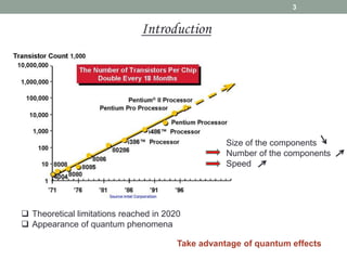
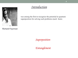
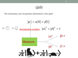
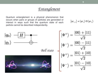
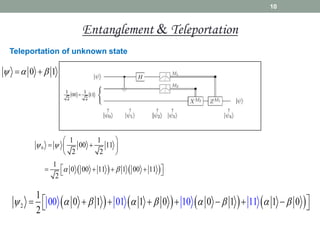
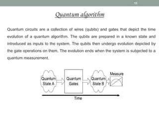
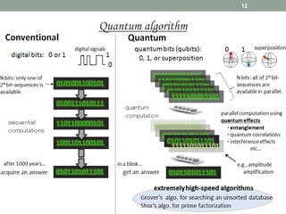
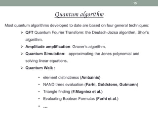
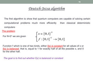
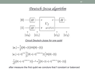
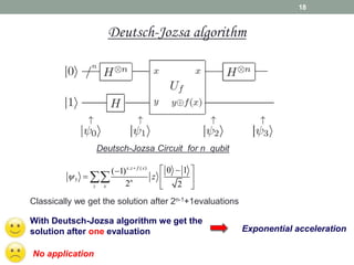
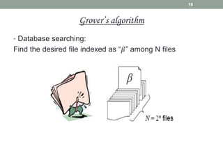
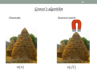
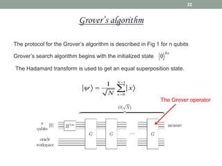
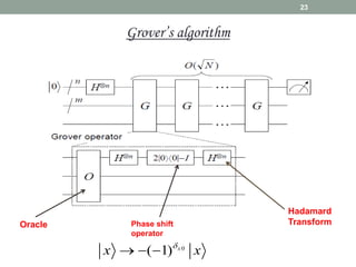
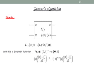
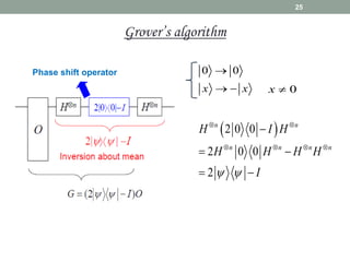
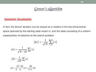
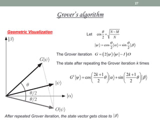
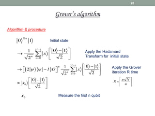
1. QUANTUM INFORMATION
1
Y. AADEL

2. 2
Outline
 Introduction
 Qubit
 Quantum gate
 No-cloning Theorem
 Entanglement
 Quantum Algorithm
 Deutsch-Jozsa algorithm
 Grover Algorithm

3. Size of the components
Number of the components
Speed
 Theoretical limitations reached in 2020
 Appearance of quantum phenomena
Take advantage of quantum effects
Introduction
3

4. 4
Introduction
Richard Feynman
was among the first to recognize the potential in quantum
superposition for solving such problems much faster.
Entanglement
Superposition

5. 5
1
0 

 

1
2
2

 

Measure
|0 >
||2
||2 |1 >
Qubit
The elementary unit of quantum information is the qubit
Normalization condition

6. 6
Qubit
Bloch sphere
cos 0 sin 1
2 2
i
e 
 
  
1
0 

 

All points on the surface of the Bloch
sphere correspond to a possible state of a
qubit. However, the possible values of a
classical bit values are restricted to two
can be identified at both poles of the
sphere.
2
{ , }
  

7. 7
Quantum gates
1 0 0 0
0 1 0 0
0 0 0 1
0 0 1 0
CNOT
 
 
 

 
 
 
† †
UU U U I
 
a b
U
c d
 
  
 
† a c
U
b d
 
 
 
  
 
 Input = output
 Reversible

8. 8
No-cloning theorem
it is impossible to create an identical copy of an arbitrary unknown quantum state
Quantum cryptography

9. 9
Bell state
Entanglement
1,2 1 2
  
 
Quantum entanglement is a physical phenomenon that
occurs when pairs or groups of particles are generated or
interact in ways such that the quantum state of each
particle cannot be described independently.

10. 10
Entanglement & Teleportation
   
0
1 1
00 11
2 2
1
0 00 11 1 00 11
2
 
 
 
 
 
 
 
   
 
       
2
1
0 1 1 0
00 01 0 1 1
2
11 0
10
        
 
       
 
0 1
  
 
Teleportation of unknown state

11. Quantum circuits are a collection of wires (qubits) and gates that depict the time
evolution of a quantum algorithm. The qubits are prepared in a known state and
introduced as inputs to the system. The qubits then undergo evolution depicted by
the gate operations on them. The evolution ends when the system is subjected to a
quantum measurement.
11
Quantum algorithm

12. 12
Quantum algorithm

13. 13
Hadamard Transform
.
.
.
u  
 
.
0,1
1
1
2 n
u x
n
x
x



Special case
 
0,1
1
0
2
n
n
n H
n
x
x





 
Quantum Parallelism

14. 14
Quantum Parallelism
Quantum Fourier Transform QFT
N
QFT 
2 i
N
e

 
 
2
0,1
1
n
i
xy
QFT N
y
x e y
N



  2n
N

Hadamard Transform is a special case of QFT

15. Most quantum algorithms developed to date are based on four general techniques:
 QFT Quantum Fourier Transform: the Deutsch-Jozsa algorithm, Shor’s
algorithm.
 Amplitude amplification: Grover’s algorithm.
 Quantum Simulation: approximating the Jones polynomial and
solving linear equations.
 Quantum Walk :
• element distinctness (Ambainis)
• NAND trees evaluation (Farhi, Goldstone, Gutmann)
• Triangle finding (F.Magniez et al.)
• Evaluating Boolean Formulas (Farhi et al.)
• …
15
Quantum algorithm

16. The first algorithm to show that quantum computers are capable of solving certain
computational problems much more efficiently than classical deterministic
computers
16
The problem
For N=2n we are given
Function f which is one of two kinds, either f(x) is constant for all values of x or
f(x) is balanced, that is, equal to 1 for exactly half of all the possible x, and 0
for the other half.
 
   
0,1
: 0,1 0,1
N
N
x
f


The goal is to find out whether f(x) is balanced or constant
Deutsch-Jozsa algorithm

17. 17
Circuit Deutsch-Jozsa for one qubit
   
1
1
0 1 0 1
2
    
     
(0) (0) (1)
2
1
1 0 1 1 0 1
2
f f f


 
     
 
 
     
 
(0) (1) (0) (1)
1 1
0 1 1 0 1 1 0 1
2
2
f f f f
H
 
  
    
after measure the first qubit we conclure that f constant or balanced
Deutsch-Jozsa algorithm

18. 18
Deutsch-Jozsa Circuit for n qubit
. ( )
3
0 1
( 1)
2 2
x z f x
n
z x
z


  

  
 

With Deutsch-Jozsa algorithm we get the
solution after one evaluation
No application
Exponential acceleration
Classically we get the solution after 2n-1+1evaluations
Deutsch-Jozsa algorithm

19. • Database searching:
Find the desired file indexed as “𝛽” among N files
19
Grover’s algorithm

20. • The problem addressed by Grover’s algorithm can be
viewed as trying to find a marked element in an
unstructured database of size N. To solve this problem a
classical algorithm need, on average O(N/2) evaluations
and O(N) in the worst case.
• But with using Grover’s algorithm, a quantum computer
can realize the same task using only O( 𝑵) evaluations.
20
Grover’s algorithm

21. 21
Grover’s algorithm
Classically Quantum search
 
O N  
O N

22. The protocol for the Grover’s algorithm is described in Fig 1 for n qubits
Grover’s search algorithm begins with the initialized state 0
n

The Hadamard transform is used to get an equal superposition state.
1
0
1 N
x
x
N



 
The Grover operator
22
Grover’s algorithm

23. Oracle
Hadamard
Transform
Phase shift
operator
0
( 1) x
x x

  
23
Grover’s algorithm

24. Oracle :
   
( ) : 0,1 0,1
n
f x 
, , ( )
x y x y f x
 
With f is a Boolean function
 
( )
0 1 0 1
1
2 2
f x
O
x x
     

 
   
   
f
U
24
Grover’s algorithm

25. Phase shift operator 0 0
x x

  0
x 
 
2 0 0
2 0 0
2
n n
n n n n
H I H
H H H H
I
 
 
   

 
 
25
Grover’s algorithm

26. Geometric Visualization
In fact, the Grover iteration can be viewed as a rotation in the two-dimensional
space spanned by the starting state vector and the state consisting of a uniform
superposition of solutions to the search problem.

1
0
1 N
x
x
N



 
1
x
N M
 


1
x
M
  
N M M
N N
  

 
26
Grover’s algorithm

27. Geometric Visualization
After repeated Grover iteration, the state vector gets close to 
cos
2
N M
N
 

Let
cos sin
2 2
 
  
 
 
2
G I O
 
 
The Grover iteration
The state after repeating the Grover iteration k times
2 1 2 1
cos sin
2 2
k k k
G     
 
   
 
   
   
27
Grover’s algorithm

28. Algorithm & procedure
0 1
n

Initial state
2 1
0
0 1
1
2
2
n
n
x
x


  
  
 
 Apply the Hadamard
Transform for initial state
 
2 1
0
0
0 1
1
2
2
2
0 1
2
n
R
n
x
I O x
x
 


  
 
   
 
 
  
  
 
 Apply the Grover
iteration R time
4
N
R

 
  
 
0
x Measure the first n qubit
28
Grover’s algorithm

29. 29
At roughly the same time that Grover published his algorithm,
Bennett, Bernstein, Brassard and Vazirani published a proof that no
quantum solution to the problem can evaluate the function fewer
than times, So Grover’s algorithm is asymptotically optimal.
( )
O N
Grover’s algorithm

30. Special case
30
00
01
10
11
1 1 1 1
00 01 10 11
2 2 2 2
    
 
2
G I O
 
 
1 1 1 1
00 01 10 11
2 2 2 2
O     
 
2
G I O
   
 
  1 1 1 1
2 00 01 10 11
2 2 2 2
G I
  
 
    
 
 
11

N M M
N N
  

 
Grover’s algorithm

31. Performance & drawback
2 1 2 1
cos sin
2 2
k k k
G     
 
   
 
   
   
2 1
2 2
k 


 sin
2
M
N

 

 
 
With
Let 𝜆 = 𝑀/𝑁 and let CI(x) denote the integer closest to the real number x.
Then repeating the Grover iteration
arccos
2arcsin
k CI


 
  
 
 
31
Grover’s algorithm

32. Performance & drawback
The success probability curve of Grover’s algorithm
The Grover’s algorithm is no longer useful when 𝜆 > 0.25
32
Grover’s algorithm

33. 33
When the Grover’s algorithm is applied to search an unordered
database, the probability of getting correct results usually decreases
with the increase of marked items.
Grover’s algorithm

34. 34
Thank You