A standard pictureof computation
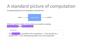
A standard abstraction of computation looks like this:
input computation output
Different specific models of computation are studied, including
Turing machines and Boolean circuits.
Key point
The entire input is provided to the computation — most typically as a
string of bits — with nothing being hidden from the computation.
3.
The query modelof computation
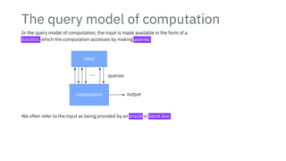
In the query model of computation, the input is made available in the form of a
function, which the computation accesses by making queries.
input
computation output
⋯ queries
We often refer to the input as being provided by an oracle or black box.
4.
The query modelof computation
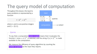
Throughout this lesson, the input to
query problems is represented by a
function
f ∶ Σ
n
→ Σ
m
where n and m are positive integers
and Σ = {0, 1}.
input
computation output
⋯ queries
Queries
To say that a computation makes a query means that it evaluates the
function f once: x ∈ Σ
n
is selected, and the string f(x) ∈ Σ
m
is made
available to the computation.
We measure the efficiency of query algorithms by counting the
number of queries to the input they require.
5.
Examples of queryproblems
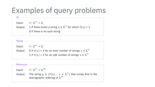
Or
Input: f ∶ Σ
n
→ Σ
Output: 1 if there exists a string x ∈ Σ
n
for which f(x) = 1
0 if there is no such string
Parity
Input: f ∶ Σ
n
→ Σ
Output: 0 if f(x) = 1 for an even number of strings x ∈ Σ
n
1 if f(x) = 1 for an odd number of strings x ∈ Σ
n
Minimum
Input: f ∶ Σ
n
→ Σ
m
Output: The string y ∈ {f(x) ∶ x ∈ Σ
n
} that comes first in the
lexicographic ordering of Σ
m
6.
Examples of queryproblems
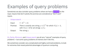
Sometimes we also consider query problems where we have a promise on the
input. Inputs that don’t satisfy the promise are considered as “don’t care”
inputs.
Unique search
Input: f ∶ Σ
n
→ Σ
Promise: There is exactly one string z ∈ Σ
n
for which f(z) = 1,
with f(x) = 0 for all strings x /
= z
Output: The string z
Or, Parity, Minimum, and Unique search are all very “natural” examples of query
problems — but some query problems of interest aren’t like this.
We sometimes consider very complicated and highly contrived problems, to look
for extremes that reveal potential advantages of quantum computing.
7.
Query gates
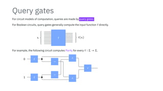
For circuitmodels of computation, queries are made by query gates.
For Boolean circuits, query gates generally compute the input function f directly.
f
x
⎧
⎪
⎪
⎪
⎪
⎪
⎨
⎪
⎪
⎪
⎪
⎪
⎩
⎫
⎪
⎪
⎪
⎬
⎪
⎪
⎪
⎭
f(x)
For example, the following circuit computes Parity for every f ∶ Σ → Σ.
f
f
0
1
¬
¬
∧
∧
∨
8.
Query gates
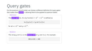
For thequantum circuit model, we choose a different definition for query gates
that makes them unitary — allowing them to be applied to quantum states.
Definition
The query gate Uf for any function f ∶ Σ
n
→ Σ
m
is defined as
Uf(∣y⟩∣x⟩) = ∣y ⊕ f(x)⟩∣x⟩
for all x ∈ Σ
n
and y ∈ Σ
m
.
Notation
The string y ⊕ f(x) is the bitwise XOR of y and f(x). For example:
001 ⊕ 101 = 100
9.
Query gates
For thequantum circuit model, we choose a different definition for query gates
that makes them unitary — allowing them to be applied to quantum states.
Definition
The query gate Uf for any function f ∶ Σ
n
→ Σ
m
is defined as
Uf(∣y⟩∣x⟩) = ∣y ⊕ f(x)⟩∣x⟩
for all x ∈ Σ
n
and y ∈ Σ
m
.
In circuit diagrammatic form Uf operates like this:
∣x⟩
∣y⟩
∣x⟩
∣y ⊕ f(x)⟩
Uf
This gate is always unitary, for any choice of the function f.
10.
Deutsch’s problem
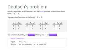
Deutsch’s problemis very simple — it’s the Parity problem for functions of the
form f ∶ Σ → Σ.
There are four functions of the form f ∶ Σ → Σ:
a f1(a)
0 0
1 0
a f2(a)
0 0
1 1
a f3(a)
0 1
1 0
a f4(a)
0 1
1 1
The functions f1 and f4 are constant while f2 and f3 are balanced.
Deutsch’s problem
Input: f ∶ Σ → Σ
Output: 0 if f is constant, 1 if f is balanced
11.
Deutsch’s problem
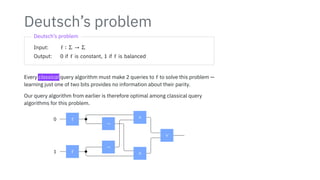
Deutsch’s problem
Input:f ∶ Σ → Σ
Output: 0 if f is constant, 1 if f is balanced
Every classical query algorithm must make 2 queries to f to solve this problem —
learning just one of two bits provides no information about their parity.
Our query algorithm from earlier is therefore optimal among classical query
algorithms for this problem.
f
f
0
1
¬
¬
∧
∧
∨
12.
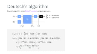
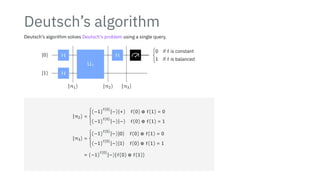
Deutsch’s algorithm
Deutsch’s algorithmsolves Deutsch’s problem using a single query.
∣0⟩
∣1⟩
H
H
Uf
H {
0 if f is constant
1 if f is balanced
∣π1⟩ ∣π2⟩ ∣π3⟩
∣π1⟩ = ∣−⟩∣+⟩ =
1
2
(∣0⟩ − ∣1⟩)∣0⟩ +
1
2
(∣0⟩ − ∣1⟩)∣1⟩
∣π2⟩ =
1
2
(∣0 ⊕ f(0)⟩ − ∣1 ⊕ f(0)⟩)∣0⟩ +
1
2
(∣0 ⊕ f(1)⟩ − ∣1 ⊕ f(1)⟩)∣1⟩
=
1
2
(−1)
f(0)
(∣0⟩ − ∣1⟩)∣0⟩ +
1
2
(−1)
f(1)
(∣0⟩ − ∣1⟩)∣1⟩
= ∣−⟩ (
(−1)
f(0)
∣0⟩ + (−1)
f(1)
∣1⟩
√
2
)
13.
Deutsch’s algorithm
Deutsch’s algorithmsolves Deutsch’s problem using a single query.
∣0⟩
∣1⟩
H
H
Uf
H {
0 if f is constant
1 if f is balanced
∣π1⟩ ∣π2⟩ ∣π3⟩
∣π2⟩ = ∣−⟩ (
(−1)
f(0)
∣0⟩ + (−1)
f(1)
∣1⟩
√
2
)
= (−1)
f(0)
∣−⟩(
∣0⟩ + (−1)
f(0)⊕f(1)
∣1⟩
√
2
)
=
⎧
⎪
⎪
⎪
⎨
⎪
⎪
⎪
⎩
(−1)
f(0)
∣−⟩∣+⟩ f(0) ⊕ f(1) = 0
(−1)
f(0)
∣−⟩∣−⟩ f(0) ⊕ f(1) = 1
14.
Deutsch’s algorithm
Deutsch’s algorithmsolves Deutsch’s problem using a single query.
∣0⟩
∣1⟩
H
H
Uf
H {
0 if f is constant
1 if f is balanced
∣π1⟩ ∣π2⟩ ∣π3⟩
∣π2⟩ =
⎧
⎪
⎪
⎪
⎨
⎪
⎪
⎪
⎩
(−1)
f(0)
∣−⟩∣+⟩ f(0) ⊕ f(1) = 0
(−1)
f(0)
∣−⟩∣−⟩ f(0) ⊕ f(1) = 1
∣π3⟩ =
⎧
⎪
⎪
⎪
⎨
⎪
⎪
⎪
⎩
(−1)
f(0)
∣−⟩∣0⟩ f(0) ⊕ f(1) = 0
(−1)
f(0)
∣−⟩∣1⟩ f(0) ⊕ f(1) = 1
= (−1)
f(0)
∣−⟩∣f(0) ⊕ f(1)⟩
15.
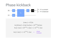
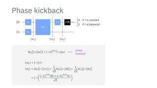
Phase kickback
∣0⟩
∣1⟩
H
H
Uf
H {
0if f is constant
1 if f is balanced
∣b ⊕ c⟩ = X
c
∣b⟩
Uf(∣b⟩∣a⟩) = ∣b ⊕ f(a)⟩∣a⟩ = (X
f(a)
∣b⟩)∣a⟩
Uf(∣−⟩∣a⟩) = (X
f(a)
∣−⟩)∣a⟩ = (−1)
f(a)
∣−⟩∣a⟩
Uf(∣−⟩∣a⟩) = (−1)
f(a)
∣−⟩∣a⟩ ⟵
phase
kickback
16.
Phase kickback
∣0⟩
∣1⟩
H
H
Uf
H {
0if f is constant
1 if f is balanced
∣π1⟩ ∣π2⟩ ∣π3⟩
Uf(∣−⟩∣a⟩) = (−1)
f(a)
∣−⟩∣a⟩ ⟵
phase
kickback
∣π1⟩ = ∣−⟩∣+⟩
∣π2⟩ = Uf(∣−⟩∣+⟩) =
1
√
2
Uf(∣−⟩∣0⟩) +
1
√
2
Uf(∣−⟩∣1⟩)
= ∣−⟩(
(−1)
f(0)
∣0⟩ + (−1)
f(1)
∣1⟩
√
2
)
17.
The Deutsch-Jozsa circuit
TheDeutsch-Jozsa algorithm extends Deutsch’s algorithm to input functions of
the form f ∶ Σ
n
→ Σ for any n ≥ 1.
The quantum circuit for the Deutsch-Jozsa algorithm looks like this:
H
H
H
H
H
H
H
Uf
∣0⟩
∣0⟩
∣0⟩
∣1⟩
⎫
⎪
⎪
⎪
⎪
⎪
⎪
⎪
⎪
⎪
⎪
⎪
⎪
⎪
⎪
⎪
⎪
⎪
⎬
⎪
⎪
⎪
⎪
⎪
⎪
⎪
⎪
⎪
⎪
⎪
⎪
⎪
⎪
⎪
⎪
⎪
⎭
y ∈ Σ
n
We can, in fact, use this circuit to solve multiple problems.
18.
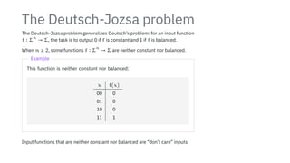
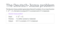
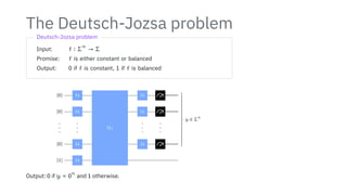
The Deutsch-Jozsa problem
TheDeutsch-Jozsa problem generalizes Deutsch’s problem: for an input function
f ∶ Σ
n
→ Σ, the task is to output 0 if f is constant and 1 if f is balanced.
When n ≥ 2, some functions f ∶ Σ
n
→ Σ are neither constant nor balanced.
Example
This function is neither constant nor balanced:
x f(x)
00 0
01 0
10 0
11 1
Input functions that are neither constant nor balanced are “don’t care” inputs.
19.
The Deutsch-Jozsa problem
TheDeutsch-Jozsa problem generalizes Deutsch’s problem: for an input function
f ∶ Σ
n
→ Σ, the task is to output 0 if f is constant and 1 if f is balanced.
Deutsch-Jozsa problem
Input: f ∶ Σ
n
→ Σ
Promise: f is either constant or balanced
Output: 0 if f is constant, 1 if f is balanced
20.
The Deutsch-Jozsa problem
Deutsch-Jozsaproblem
Input: f ∶ Σ
n
→ Σ
Promise: f is either constant or balanced
Output: 0 if f is constant, 1 if f is balanced
H
H
H
H
H
H
H
Uf
∣0⟩
∣0⟩
∣0⟩
∣1⟩
⎫
⎪
⎪
⎪
⎪
⎪
⎪
⎪
⎪
⎪
⎪
⎪
⎪
⎪
⎪
⎪
⎪
⎪
⎬
⎪
⎪
⎪
⎪
⎪
⎪
⎪
⎪
⎪
⎪
⎪
⎪
⎪
⎪
⎪
⎪
⎪
⎭
y ∈ Σ
n
Output: 0 if y = 0
n
and 1 otherwise.
21.
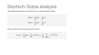
Deutsch-Jozsa analysis
The Hadamardoperation works like this on standard basis states:
H∣0⟩ =
1
√
2
∣0⟩ +
1
√
2
∣1⟩
H∣1⟩ =
1
√
2
∣0⟩ −
1
√
2
∣1⟩
We can express these two equations as one:
H∣a⟩ =
1
√
2
∣0⟩ +
1
√
2
(−1)
a
∣1⟩ =
1
√
2
∑
b∈{0,1}
(−1)
ab
∣b⟩
22.
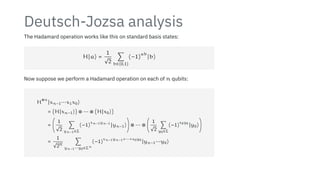
Deutsch-Jozsa analysis
The Hadamardoperation works like this on standard basis states:
H∣a⟩ =
1
√
2
∑
b∈{0,1}
(−1)
ab
∣b⟩
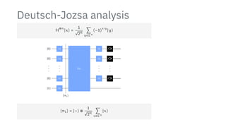
Now suppose we perform a Hadamard operation on each of n qubits:
H
⊗n
∣xn−1⋯x1x0⟩
= (H∣xn−1⟩) ⊗ ⋯ ⊗ (H∣x0⟩)
= (
1
√
2
∑
yn−1∈Σ
(−1)
xn−1yn−1
∣yn−1⟩) ⊗ ⋯ ⊗ (
1
√
2
∑
y0∈Σ
(−1)
x0y0
∣y0⟩)
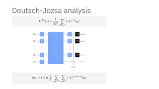
=
1
√
2n
∑
yn−1⋯y0∈Σn
(−1)
xn−1yn−1+⋯+x0y0
∣yn−1⋯y0⟩
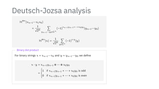
Deutsch-Jozsa analysis
The probabilityfor the measurements to give y = 0
n
is
p(0
n
) =
2
2
2
2
2
2
2
2
2
2
1
2n ∑
x∈Σn
(−1)
f(x)
2
2
2
2
2
2
2
2
2
2
2
= {
1 if f is constant
0 if f is balanced
The Deutsch-Jozsa algorithm therefore solves the Deutsch-Jozsa problem
without error with a single query.
Any deterministic algorithm for the Deutsch-Jozsa problem must at least
2
n−1
+ 1 queries.
A probabilistic algorithm can, however, solve the Deutsch-Jozsa problem using
just a few queries:
1. Choose k input strings x
1
, . . . , x
k
∈ Σ
n
uniformly at random.
2. If f(x
1
) = ⋯ = f(x
k
), then answer 0 (constant), else answer 1 (balanced).
If f is constant, this algorithm is correct with probability 1.
If f is balanced, this algorithm is correct with probability 1 − 2
−k+1
.
28.
The Bernstein-Vazirani problem
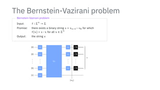
Bernstein-Vaziraniproblem
Input: f ∶ Σ
n
→ Σ
Promise: there exists a binary string s = sn−1⋯s0 for which
f(x) = s ⋅ x for all x ∈ Σ
n
Output: the string s
H
H
H
H
H
H
H
Uf
∣0⟩
∣0⟩
∣0⟩
∣1⟩
⎫
⎪
⎪
⎪
⎪
⎪
⎪
⎪
⎪
⎪
⎪
⎪
⎪
⎪
⎪
⎪
⎪
⎪
⎬
⎪
⎪
⎪
⎪
⎪
⎪
⎪
⎪
⎪
⎪
⎪
⎪
⎪
⎪
⎪
⎪
⎪
⎭
s
∣π3⟩
29.
The Bernstein-Vazirani problem
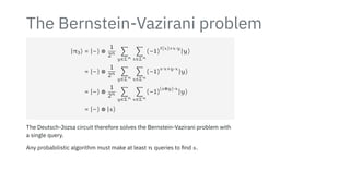
∣π3⟩= ∣−⟩ ⊗
1
2n ∑
y∈Σn
∑
x∈Σn
(−1)
f(x)+x⋅y
∣y⟩
= ∣−⟩ ⊗
1
2n ∑
y∈Σn
∑
x∈Σn
(−1)
s⋅x+y⋅x
∣y⟩
= ∣−⟩ ⊗
1
2n ∑
y∈Σn
∑
x∈Σn
(−1)
(s⊕y)⋅x
∣y⟩
= ∣−⟩ ⊗ ∣s⟩
The Deutsch-Jozsa circuit therefore solves the Bernstein-Vazirani problem with
a single query.
Any probabilistic algorithm must make at least n queries to find s.
30.
Simon’s problem
Simon’s problem
Input:A function f ∶ Σ
n
→ Σ
m
Promise: There exists a string s ∈ Σ
n
such that
[f(x) = f(y)] ⇔ [(x = y) or (x ⊕ s = y)]
for all x, y ∈ Σ
n
Output: The string s
Case 1: s = 0
n
The condition in the promise simplifies to
[f(x) = f(y)] ⇔ [x = y]
This is equivalent to f being one-to-one.
31.
Simon’s problem
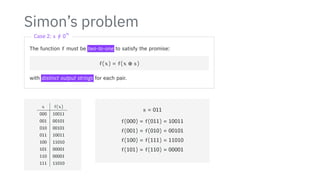
Case 2:s /
= 0
n
The function f must be two-to-one to satisfy the promise:
f(x) = f(x ⊕ s)
with distinct output strings for each pair.
x f(x)
000 10011
001 00101
010 00101
011 10011
100 11010
101 00001
110 00001
111 11010
s = 011
f(000) = f(011) = 10011
f(001) = f(010) = 00101
f(100) = f(111) = 11010
f(101) = f(110) = 00001
32.
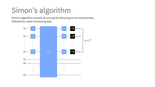
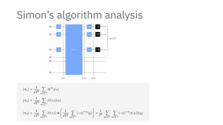
Simon’s algorithm
Simon’s algorithmconsists of running the following circuit several times,
followed by a post-processing step.
H
H
H
H
H
H
Uf
∣0⟩
∣0⟩
∣0⟩
∣0⟩
∣0⟩
∣0⟩
⎫
⎪
⎪
⎪
⎪
⎪
⎪
⎪
⎪
⎪
⎪
⎪
⎪
⎪
⎪
⎪
⎪
⎪
⎬
⎪
⎪
⎪
⎪
⎪
⎪
⎪
⎪
⎪
⎪
⎪
⎪
⎪
⎪
⎪
⎪
⎪
⎭
y ∈ Σ
n
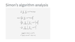
Simon’s algorithm analysis
p(y)=
1
22n
∑
z∈range(f)
2
2
2
2
2
2
2
2
2
2
2
2
∑
x∈f−1({z})
(−1)
x⋅y
2
2
2
2
2
2
2
2
2
2
2
2
2
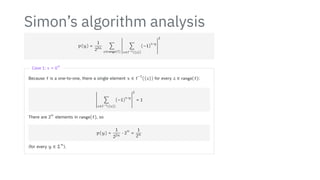
Case 1: s = 0
n
Because f is a one-to-one, there a single element x ∈ f
−1
({z}) for every z ∈ range(f):
2
2
2
2
2
2
2
2
2
2
2
2
∑
x∈f−1({z})
(−1)
x⋅y
2
2
2
2
2
2
2
2
2
2
2
2
2
= 1
There are 2
n
elements in range(f), so
p(y) =
1
22n
⋅ 2
n
=
1
2n
(for every y ∈ Σ
n
).
36.
Simon’s algorithm analysis
p(y)=
1
22n
∑
z∈range(f)
2
2
2
2
2
2
2
2
2
2
2
2
∑
x∈f−1({z})
(−1)
x⋅y
2
2
2
2
2
2
2
2
2
2
2
2
2
Case 2: s /
= 0
n
There are two strings in the set f
−1
({z}) for each z ∈ range(f); if w ∈ f
−1
({z}) either one
of them, then w ⊕ s is the other.
2
2
2
2
2
2
2
2
2
2
2
2
∑
x∈f−1({z})
(−1)
x⋅y
2
2
2
2
2
2
2
2
2
2
2
2
2
=
2
2
2
2
2
2
(−1)
w⋅y
+ (−1)
(w⊕s)⋅y2
2
2
2
2
2
2
=
2
2
2
2
2
2
1 + (−1)
s⋅y2
2
2
2
2
2
2
= {
4 s ⋅ y = 0
0 s ⋅ y = 1
There are 2
n−1
elements in range(f), so
p(y) =
1
22n
∑
z∈range(f)
2
2
2
2
2
2
2
2
2
2
2
2
∑
x∈f−1({z})
(−1)
x⋅y
2
2
2
2
2
2
2
2
2
2
2
2
2
=
⎧
⎪
⎪
⎪
⎨
⎪
⎪
⎪
⎩
1
2n−1 s ⋅ y = 0
0 s ⋅ y = 1
37.
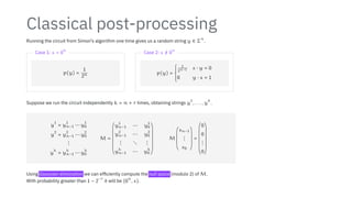
Classical post-processing
Running thecircuit from Simon’s algorithm one time gives us a random string y ∈ Σ
n
.
Case 1: s = 0
n
p(y) =
1
2n
Case 2: s /
= 0
n
p(y) =
⎧
⎪
⎪
⎪
⎨
⎪
⎪
⎪
⎩
1
2n−1 s ⋅ y = 0
0 y ⋅ s = 1
Suppose we run the circuit independently k = n + r times, obtaining strings y
1
, . . . , y
k
.
y
1
= y
1
n−1 ⋯ y
1
0
y
2
= y
2
n−1 ⋯ y
2
0
⋮
y
k
= y
k
n−1 ⋯ y
k
0
M =
⎛
⎜
⎜
⎜
⎜
⎜
⎜
⎜
⎜
⎜
⎜
⎜
⎜
⎝
y
1
n−1 ⋯ y
1
0
y
2
n−1 ⋯ y
2
0
⋮ ⋱ ⋮
y
k
n−1 ⋯ y
k
0
⎞
⎟
⎟
⎟
⎟
⎟
⎟
⎟
⎟
⎟
⎟
⎟
⎟
⎠
M
⎛
⎜
⎜
⎜
⎜
⎜
⎜
⎝
sn−1
⋮
s0
⎞
⎟
⎟
⎟
⎟
⎟
⎟
⎠
=
⎛
⎜
⎜
⎜
⎜
⎜
⎜
⎜
⎜
⎜
⎜
⎜
⎜
⎝
0
0
⋮
0
⎞
⎟
⎟
⎟
⎟
⎟
⎟
⎟
⎟
⎟
⎟
⎟
⎟
⎠
Using Gaussian elimination we can efficiently compute the null space (modulo 2) of M.
With probability greater than 1 − 2
−r
it will be {0
n
, s}.
38.
Classical difficulty
Any probabilisticalgorithm making fewer than 2
n/2−1
− 1 queries will fail to
solve Simon’s problem with probability at least 1/2.
• Simon’s algorithm solves Simon’s problem with a linear number of queries.
• Every classical algorithm for Simon’s problem requires an
exponential number of queries.


![Simon’s problem
Simon’s problem
Input: A function f ∶ Σ
n
→ Σ
m
Promise: There exists a string s ∈ Σ
n
such that
[f(x) = f(y)] ⇔ [(x = y) or (x ⊕ s = y)]
for all x, y ∈ Σ
n
Output: The string s
Case 1: s = 0
n
The condition in the promise simplifies to
[f(x) = f(y)] ⇔ [x = y]
This is equivalent to f being one-to-one.](https://image.slidesharecdn.com/05-quantum-query-algorithms-slides-251217005459-c553d86b/85/05-Quantum-query-algorithms-slides-pdfnxjxjxjx-30-320.jpg)


![Prac 9 Therapeutic Ex [Lower].pdfdnxjzjsj](https://cdn.slidesharecdn.com/ss_thumbnails/prac9therapeuticexlower-251217074550-6c2c6de8-thumbnail.jpg?width=640&height=640&fit=bounds)


