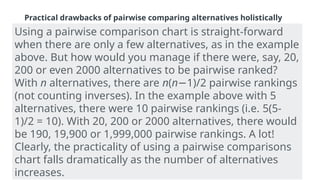
The document explains the even swaps method and pairwise comparison charts as tools for ranking alternatives, particularly in decision-making scenarios. It illustrates the method through an example of ranking job candidates and highlights the practicality challenges of using pairwise comparisons as the number of alternatives increases. The even swap method allows for adjustments between objectives, making trade-offs explicit and justifiable, while also emphasizing that making difficult choices remains a fundamental part of the decision-making process.

1. Even Swaps Method

2. Pairwise comparison charts
• A simple way to implement the pairwise comparison method is to use
a pairwise comparison chart (sometimes called a paired comparison
chart). As an illustration, imagine you want to hire someone for a job
from a short-list of five candidates, who you want to rank from first to
fifth, i.e. best to worst.
• Start by creating a pairwise comparison table, as in Table 1 below,
with the candidates listed down the left hand-side and also along the
top.

3. Neha Peter Sajid Bao Susanna
Neha –
Peter –
Sajid –
Bao –
Susanna –
Neha Peter Sajid Bao Susanna
Neha – 1 1 0 0,5
Peter 0 – 0 1 0
Sajid 0 1 – 1 0
Bao 1 0 0 – 0
Susanna 0,5 1 1 1 –

4. After having completed all 10 pairwise comparisons, for each
candidate add up their points across the row to get their total
scores:
•Neha: 1 + 1 + 0 + 0.5 = 2.5
•Peter: 0 + 0 + 1 + 0 = 1
•Sajid: 0 + 1 + 1 + 0 = 2
•Bao: 1 + 0 + 0 + 0 = 1
•Susan: 0.5 + 1 + 1 + 1 = 3.5
Use the candidates’ total scores to rank them. We can see that
Susan, with 3.5 points, is in 1st place, followed by Neha (2nd),
Sajid (3rd), and Peter and Bao are tied for 4th equal.

5. Practical drawbacks of pairwise comparing alternatives holistically
Using a pairwise comparison chart is straight-forward
when there are only a few alternatives, as in the example
above. But how would you manage if there were, say, 20,
200 or even 2000 alternatives to be pairwise ranked?
With n alternatives, there are n(n 1)/2
− pairwise rankings
(not counting inverses). In the example above with 5
alternatives, there were 10 pairwise rankings (i.e. 5(5-
1)/2 = 10). With 20, 200 or 2000 alternatives, there would
be 190, 19,900 or 1,999,000 pairwise rankings. A lot!
Clearly, the practicality of using a pairwise comparisons
chart falls dramatically as the number of alternatives
increases.

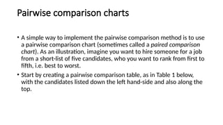
6. The concept
• Firstly, a fundamental principle of decision making: if all alternatives are
rated equally for a given objective, then you can ignore that objective in
making your decision [1].
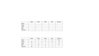
• “The even swap method provides a way to adjust the consequences of
different alternatives in order to render them equivalent in terms of a given
objective. Thus this objective becomes irrelevant. As its name implies, an
even swap increases the value of an alternative in terms of one objective
while decreasing its value by an equivalent amount in terms of another
objective. In essence, the even swap method is a form of bartering – it forces
you to think about the value of one objective in terms of another” [2].

7. • Let’s say strategic alternatives A, B and C mentioned above deliver the
following outcomes. Note that these are purely illustrative numbers.
• A: creates 100 new jobs, offsets zero Carbon, delivers negative $10
million economic profit
• B: creates 10 new jobs, offsets 10,000 tons of Carbon, delivers zero
economic profit
• C: creates zero new jobs, offsets zero Carbon, delivers positive $10
million economic profit

8. Alternative New Jobs Carbon Profit
A 100 0 -10 million
B 10 10000 0
C 0 0 10 million

9. • Step 1 of the even swap method: determine what change is necessary
to cancel an objective. Let’s cancel economic profit.
• After some deliberation, we determine that we value gaining $1
million as equivalent to reducing 1,000 tons of Carbon. We can set all
strategies A and C to the economic profit of B, i.e. zero economic
profit, by doing an even swap of each $1m for 1,000 tons of Carbon.

10. Alternative New Jobs Carbon Profit
A 100 Creates 10000 0
B 10 Offsets 10000 0
C 0 Offsets 10000 0
This would then produce:
•A: creates 100 new jobs, creates 10,000 tons of Carbon
•B: creates 10 new jobs, offsets 10,000 tons Carbon
•C: creates zero new jobs, offsets 10,000 tons Carbon
Now, it is clear that B is a better strategy than C, since they both offset the same amount of
Carbon, but creates new jobs, so we can eliminate C.

11. But, still we have A and B to decide between. A second even swap is
called for. This time between jobs and Carbon. We make another
subjective choice by saying that each job created is worth 200 tons of
offset Carbon. So, if we set B to 100 new jobs, we are creating an extra
90 new jobs for B, which costs us 200 x 90 tons of Carbon. This leads A
and B to both create the equivalent of 100 jobs, but now B’s Carbon
offset becomes a negative 8,000 (or 8,000 tons created; this comes
from the original 10,000 minus the cost of 200 x 90).

12. Alternative New Jobs Carbon
A 100 Creates 10000
B 10 Offsets 10000
Alternative New Jobs Carbon
A 100 Creates 10000
B 100 Offsets 10000 – Creates 90*200
Alternative New Jobs Carbon
A 100 Creates 10000
B 100 Creates 8000

13. • A: creates 100 new jobs, creates 10,000 tons of Carbon
• B: creates 100 new jobs, creates 8,000 tons Carbon
At this point, A and B can be compared on a single variable, i.e. Carbon
offset. They are both negative with A creating 10,000 tons (nothing’s
changed) and with B now creating 8,000 tons. So, by two applications
of the even swap method, we have determined that B is the better
overall strategy.

14. • In closing, “The even swap method will not make complex decisions
easy; you’ll still have to make hard choices about the values you set
and the trades you make. What it does provide is a reliable
mechanism for making trades and a coherent framework in which to
make them” [1].

15. • Postscript 1: if this technique reminds you of the Benjamin Franklin
technique, you’re quite right as the even swap method was informed by this.
• Postscript 2: if you’re wondering why not just use weightings for each of the
objectives, then I should remind you of a great quote by
Kahneman: “Hypothesis testing can be completely contaminated if the
organization knows the answer that the leader wants to get” [3].
• Weighting the objectives is a sure-fire way of manipulating the process to
achieve the outcome you want – I’ve seen this more than once at my
clients. The even swap method also has some vulnerability to this form of
manipulation, sigh, but it is better in it that forces swaps to be explicitly
defined and hence justified.

16. References:
• [1] “Even Swaps: A Rational Method for Making Trade-offs”,
Hammond, Keeney and Raiffa
• [2] “Smart Choices”, Hammond, Keeney and Raiffa
• [3] “Strategic decisions: When can you trust your gut?”, McKinsey
Quarterly
• [4] Pairwise comparison method & pairwise ranking | 1000minds

17. Address Floor space
(m2
)
Quality of work
facilities
Quality of local
amenities
Quality of
public transport
Monthly rent
($)
15 Pleasant Point 300 medium medium low 5500
6 Yellow Brick Road 400 medium medium medium 5000
23 Happy Valley 400 high low high 6000
77 Sunshine Lane 550 low medium high 7500
50 Heavenly Way 560 low medium low 9000

18. Address Floor space (m2
) Quality of work
facilities
Quality of local
amenities
Quality of public
transport
Monthly rent ($)
15 Pleasant Point 300 medium medium low 5500
6 Yellow Brick
Road 400 medium medium medium 5000
23 Happy Valley 400 high low high 6000
77 Sunshine Lane 550 low medium high 7500
50 Heavenly Way 560 low medium low 9000

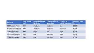
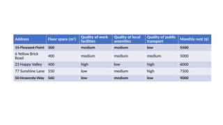
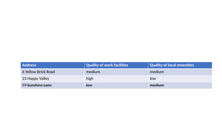
19. Address
Floor space
(m2
)
Quality of
work facilities
Quality of
local
amenities
Quality of
public
transport
Monthly rent
($)
6 Yellow Brick
Road
400 medium medium medium [high] 5000 [6000]
23 Happy
Valley
400 high low high 6000
77 Sunshine
Lane 550 [400] low medium high 7500 [6000]

20. Address Quality of work facilities Quality of local amenities
6 Yellow Brick Road medium medium
23 Happy Valley high low
77 Sunshine Lane low medium