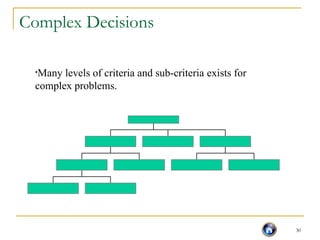
Learning Objectives
Students willbe able to:
1. Use the multifactor evaluation process in making
decisions that involve a number of factors, where
importance weights can be assigned.
2. Understand the use of the analytic hierarchy process
in decision making.
3. Contrast multifactor evaluation with the analytic
hierarchy process.
Introduction
Multifactor decisionmaking involves individuals
subjectively and intuitively considering various
factors prior to making a decision.
Multifactor evaluation process (MFEP) is a
quantitative approach that gives weights to each
factor and scores to each alternative.
Analytic hierarchy process (AHP) is an approach
designed to quantify the preferences for various
factors and alternatives.
5.
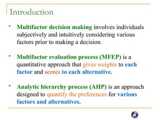
Multifactor Evaluation Process
FactorImportance (weight)
Salary 0.3
Career
Advancement
0.6
Location 0.1
Example: Steve: considering employment with 3 companies.
Determined 3 criterias important to him,
assigned each factor a weight.
Weights should sum to 1
6.
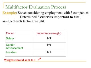
Multifactor Evaluation Process
FactorImportance
(weight)
AA
Co.
EDS,
LTD.
PW,
Inc.
Salary 0.3 0.7 0.8 0.9
Career
Advancement
0.6 0.9 0.7 0.6
Location 0.1 0.6 0.8 0.9
Weights should sum to 1
Steve evaluated the various factors on a 0 to 1
scale for each of these jobs.
Score Table
7.
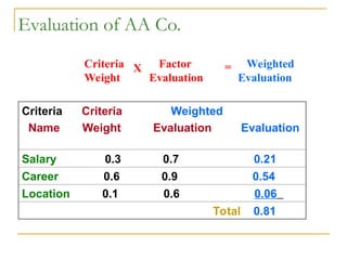
Evaluation of AACo.
Criteria Criteria Weighted
Name Weight Evaluation Evaluation
Salary 0.3 0.7 0.21
Career 0.6 0.9 0.54
Location 0.1 0.6 0.06
Total 0.81
Criteria Factor Weighted
Weight Evaluation Evaluation
X =
8.
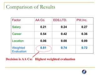
Comparison of Results
FactorAA Co. EDS,LTD. PW,Inc.
Salary 0.21 0.24 0.27
Career 0.54 0.42 0.36
Location 0.06 0.08 0.09
Weighted
Evaluation
0.81 0.74 0.72
Decision is AA Co: Highest weighted evaluation
9.
9
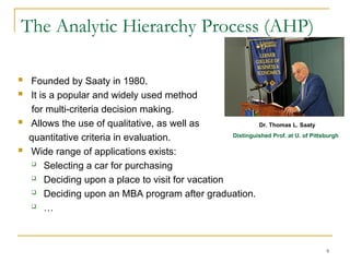
The Analytic HierarchyProcess (AHP)
Founded by Saaty in 1980.
It is a popular and widely used method
for multi-criteria decision making.
Allows the use of qualitative, as well as
quantitative criteria in evaluation.
Wide range of applications exists:
Selecting a car for purchasing
Deciding upon a place to visit for vacation
Deciding upon an MBA program after graduation.
…
Dr. Thomas L. Saaty
Distinguished Prof. at U. of Pittsburgh
10.
10
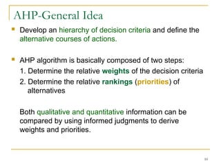
AHP-General Idea
Developan hierarchy of decision criteria and define the
alternative courses of actions.
AHP algorithm is basically composed of two steps:
1. Determine the relative weights of the decision criteria
2. Determine the relative rankings (priorities) of
alternatives
Both qualitative and quantitative information can be
compared by using informed judgments to derive
weights and priorities.
11.
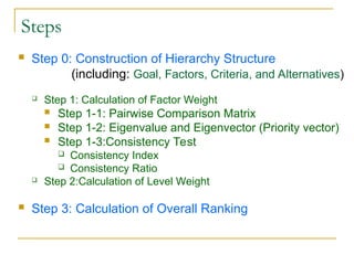
Steps
Step 0:Construction of Hierarchy Structure
(including: Goal, Factors, Criteria, and Alternatives)
Step 1: Calculation of Factor Weight
Step 1-1: Pairwise Comparison Matrix
Step 1-2: Eigenvalue and Eigenvector (Priority vector)
Step 1-3:Consistency Test
Consistency Index
Consistency Ratio
Step 2:Calculation of Level Weight
Step 3: Calculation of Overall Ranking
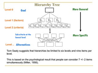
12.
C1 C2 C3
C11C12 C13
More Specific
Alternatives
More General
Goal
C21 C22 C31 C32 C33
Sub-criteria at the
lowest level
Hierarchy Tree
Level 0
Level 1 (factors)
Level 2 (criteria)
Level ..
Tom Saaty suggests that hierarchies be limited to six levels and nine items per
Tom Saaty suggests that hierarchies be limited to six levels and nine items per
level.
level.
This is based on the psychological result that people can consider 7 +/- 2 items
This is based on the psychological result that people can consider 7 +/- 2 items
simultaneously (Miller, 1956).
simultaneously (Miller, 1956).
13.
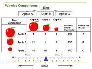
Pairwise Comparisons
Size
Apple AApple B Apple C
Size
Comparison
Apple A Apple B Apple C
Apple A 1 2 6 6/10 A
Apple B 1/2 1 3 3/10 B
Apple C 1/6 1/3 1 1/10 C
Resulting
Priority
Eigenvector
Relative Size
of Apple
Criteria #1 Criteria #2
1
Intensity of
Importance
2 3 4 5 6 8
7 9
9 8 7 6 5 3
4 2
14.
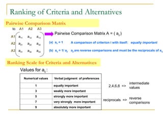
Pairwise Comparison Matrix
PairwiseComparison Matrix A = ( aij )
a33
a32
a31
A3
a32
a22
a21
A2
a13
a12
a11
A1
A3
A2
A1
to
Values for aij :
Numerical values Verbal judgment of preferences
1 equally important
3 weakly more important
5 strongly more important
7 very strongly more important
9 absolutely more important
2,4,6,8 =>
reciprocals =>
intermediate
values
reverse
comparisons
Ranking of Criteria and Alternatives
Ranking Scale for Criteria and Alternatives
(a) aii = 1 A comparison of criterion i with itself: equally important
(b) aij = 1/ aji aji are reverse comparisons and must be the reciprocals of aij
15.
15
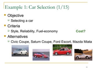
Example 1: CarSelection (1/15)
Objective
Selecting a car
Criteria
Style, Reliability, Fuel-economy Cost?
Alternatives
Civic Coupe, Saturn Coupe, Ford Escort, Mazda Miata
16.
16
Hierarchy tree
S tyleReliability Fuel E conom y
S electing
a New Car
Civic Saturn Escort Miata
Example 1: Car Selection (2/15)
17.
17
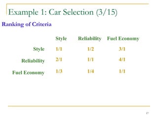
Ranking of Criteria
StyleReliability Fuel Economy
Style
Reliability
Fuel Economy
1/1 1/2 3/1
2/1 1/1 4/1
1/3 1/4 1/1
Example 1: Car Selection (3/15)
18.
18
Ranking of Priorities
Consider [Ax = x] where
A is the comparison matrix of size n×n, for n criteria, also called the priority
matrix.
x is the Eigenvector of size n×1, also called the priority vector.
is the Eigenvalue, > n.
To find the ranking of priorities, namely the Eigen Vector X:
1) Normalize the column entries by dividing each entry by the sum of the column.
2) Take the overall row averages.
0.30 0.29 0.38
0.60 0.57 0.50
0.10 0.14 0.13
Column sums 3.33 1.75 8.00 1.00 1.00 1.00
A=
1 0.5 3
2 1 4
0.33 0.25 1.0
Normalized
Column Sums
Row
Averages
0.3196
0.5584
0.1220
Priority vector
X=
Example 1: Car Selection (4/15)
Example 1: Car Selection (4/15)
Pairwise Comp. Matrix Norm. Pairwise Comp. Matrix
19.
19
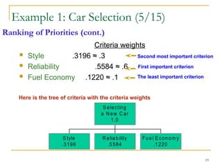
Criteria weights
Style.3196 ≈ .3
Reliability .5584 ≈ .6
Fuel Economy .1220 ≈ .1
S tyle
.3196
R eliability
.5584
Fuel E conom y
.1220
S electing
a N ew C ar
1.0
First important criterion
Second most important criterion
Here is the tree of criteria with the criteria weights
The least important criterion
Ranking of Priorities (cont.)
Example 1: Car Selection (5/15)
20.
20
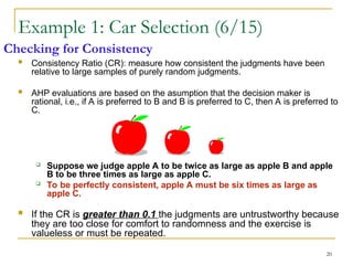
Checking for Consistency
Consistency Ratio (CR): measure how consistent the judgments have been
relative to large samples of purely random judgments.
AHP evaluations are based on the asumption that the decision maker is
rational, i.e., if A is preferred to B and B is preferred to C, then A is preferred to
C.
Suppose we judge apple A to be twice as large as apple B and apple
B to be three times as large as apple C.
To be perfectly consistent, apple A must be six times as large as
apple C.
If the CR is greater than 0.1 the judgments are untrustworthy because
they are too close for comfort to randomness and the exercise is
valueless or must be repeated.
Example 1: Car Selection (6/15)
21.
21
Calculation of ConsistencyRatio
0.30
0.60
0.10
1 0.5 3
2 1 4
0.333 0.25 1.0
0.90
1.60
0.35
=
A x Ax x
=
A x Ax x
Consistency index (CI) is found by
The next stage is to calculate , Consistency Index (CI) and the
Consistency Ratio (CR).
Consider [Ax = x] where x is the Eigenvector.
= =
0.30
0.60
0.10
A x Ax x
Example 1: Car Selection (7/15)
Consistency Vector =
0.90/0.30
1.60/0.60
0.35/0.10
06
.
3
3
5
.
3
67
.
2
0
.
3
3.00
2.67
3.50
=
03
.
0
1
3
3
06
.
3
1
n
n
CI
Note: This is just an approximate method to determine value of λ
22.
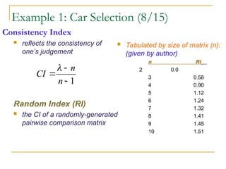
Consistency Index
reflectsthe consistency of
one’s judgement
Random Index (RI)
the CI of a randomly-generated
pairwise comparison matrix
Tabulated by size of matrix (n):
(given by author)
n RI
2 0.0
3 0.58
4 0.90
5 1.12
6 1.24
7 1.32
8 1.41
9 1.45
10 1.51
Example 1: Car Selection (8/15)
1
n
n
CI
23.
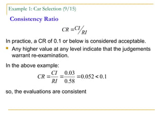
Consistency Ratio
In practice,a CR of 0.1 or below is considered acceptable.
Any higher value at any level indicate that the judgements
warrant re-examination.
RI
CI
CR
Example 1: Car Selection (9/15)
In the above example:
so, the evaluations are consistent
1
.
0
052
.
0
58
.
0
03
.
0
RI
CI
CR
25
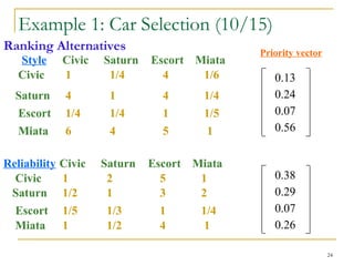
Fuel Economy Civic
Saturn
Escort
Miata
Miata
34
27
24
28
113
Miles/gallonNormalized
.30
.24
.21
.25
1.0
Ranking Alternatives (cont.)
! Since fuel economy is a quantitative measure, fuel consumption ratios
can be used to determine the relative ranking of alternatives; however
this is not obligatory. Pairwise comparisons may still be used in some
cases.
Example 1: Car Selection (11/15)
Ranking Alternatives (cont.)
Example 1: Car Selection (11/15)
26.
26
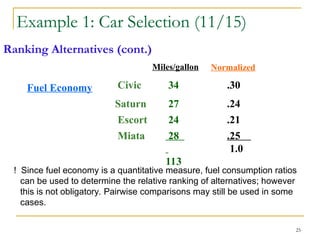
Civic 0.13
Saturn 0.24
Escort0.07
Miata 0.56
Civic 0.38
Saturn 0.29
Escort 0.07
Miata 0.26
Civic 0.30
Saturn 0.24
Escort 0.21
Miata 0.25
Style
0.30
Reliability
0.60
Fuel Economy
0.10
Selecting a New Car
1.00
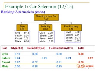
Ranking Alternatives (cont.)
Example 1: Car Selection (12/15)
Car Style(0.3) Reliability(0.6) Fuel Economy(0.1) Total
Civic 0.13 0.38 0.30 0.30
Saturn 0.24 0.29 0.24 0.27
Escort 0.07 0.07 0.21 0.08
Miata 0.56 0.26 0.25 0.35 largest
27.
27
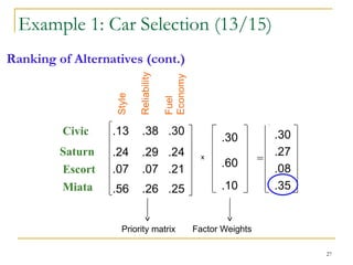
Ranking of Alternatives(cont.)
Civic
Escort
Miata
Miata
Saturn
.13 .38 .30
.24 .29 .24
.07 .07 .21
.56 .26 .25
x
.30
.60
.10
=
.30
.27
.08
.35
Factor Weights
Priority matrix
Example 1: Car Selection (13/15)
28.
28
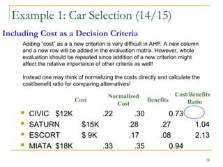
Including Cost asa Decision Criteria
CIVIC $12K .22 .30 0.73
SATURN $15K .28 .27 1.04
ESCORT $ 9K .17 .08 2.13
MIATA $18K .33 .35 0.94
Cost
Normalized
Cost
Cost/Benefits
Ratio
Adding “cost” as a a new criterion is very difficult in AHP. A new column
and a new row will be added in the evaluation matrix. However, whole
evaluation should be repeated since addition of a new criterion might
affect the relative importance of other criteria as well!
Instead one may think of normalizing the costs directly and calculate the
cost/benefit ratio for comparing alternatives!
Benefits
Example 1: Car Selection (14/15)
29.
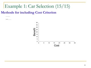
Methods for includingCost Criterion
Use graphical representations to make trade-offs.
Calculate cost/benefit ratios
Use linear programming
Use seperate benefit and cost trees and then combine the results
29
Civic
Escort
Saturn
Miata
Example 1: Car Selection (15/15)
Civic
Escort
Saturn
Miata
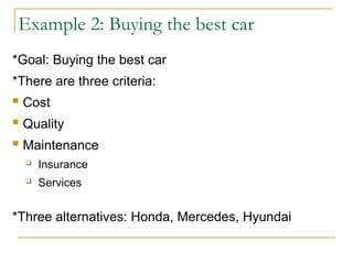
*Goal: Buying thebest car
*There are three criteria:
Cost
Quality
Maintenance
Insurance
Services
*Three alternatives: Honda, Mercedes, Hyundai
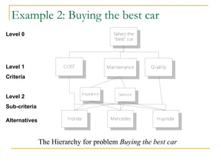
Example 2: Buying the best car
32.
Select the
"best" car
COSTMaintenance Quality
Service
Insurance
Honda Mercedes Huyndai
Level 0
Level 1
Criteria
Level 2
Sub-criteria
Alternatives
The Hierarchy for pro
oblem Buying the best car
Example 2: Buying the best car
33.
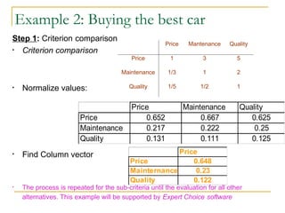
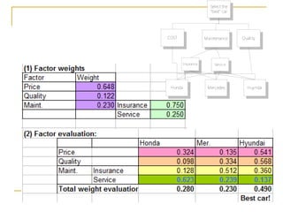
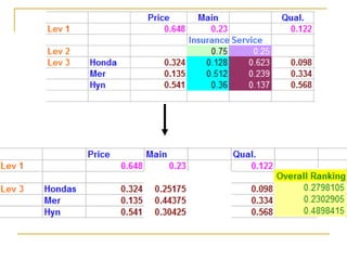
Step 1: Criterioncomparison
• Criterion comparison
• Normalize values:
• Find Column vector
• The process is repeated for the sub-criteria until the evaluation for all other
alternatives. This example will be supported by Expert Choice software
Price Mantenance Quality
Price 1 3 5
Maintenance 1/3 1 2
Quality 1/5 1/2 1
Price Maintenance Quality
Price 0.652 0.667 0.625
Maintenance 0.217 0.222 0.25
Quality 0.131 0.111 0.125
Example 2: Buying the best car
Price
Price 0.648
Mainternance 0.23
Quality 0.122
34.
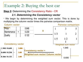
Step 2: Determiningthe Consistency Ratio - CR
2.1. Determining the Consistency vector
• We begin by determining the weighted sum vector. This is done by
multiplying the column vector times the pairwise comparison matrix.
Column vector: Pairwise comparison
matrix:
Price 0.648
Mainternance = 0.230
Quality 0.122
1 3 5
1/3 1 2
1/5 1/2 1
Example 2: Buying the best car
X
Weighted sum vector
Consistency vector =
Weighted sum vector/ Column vector
Consistency vector
1.948
0.690
35.
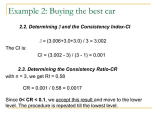
2.2. Determining and the Consistency Index-CI
= (3.006+3.0+3.0) / 3 = 3.002
The CI is:
CI = (3.002 - 3) / (3 - 1) = 0.001
2.3. Determining the Consistency Ratio-CR
with n = 3, we get RI = 0.58
CR = 0.001 / 0.58 = 0.0017
Since 0< CR < 0.1, we accept this result and move to the lower
level. The procedure is repeated till the lowest level.
Example 2: Buying the best car
36.
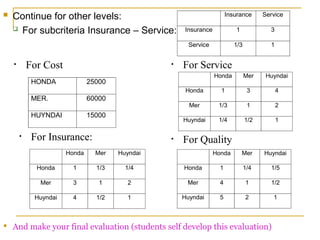
Continue forother levels:
For subcriteria Insurance – Service:
Insurance Service
Insurance 1 3
Service 1/3 1
HONDA 25000
MER. 60000
HUYNDAI 15000
Honda Mer Huyndai
Honda 1 1/3 1/4
Mer 3 1 2
Huyndai 4 1/2 1
• For Cost
• For Insurance:
Honda Mer Huyndai
Honda 1 3 4
Mer 1/3 1 2
Huyndai 1/4 1/2 1
• For Service
Honda Mer Huyndai
Honda 1 1/4 1/5
Mer 4 1 1/2
Huyndai 5 2 1
• For Quality
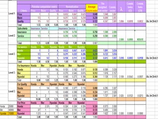
And make your final evaluation (students self develop this evaluation)
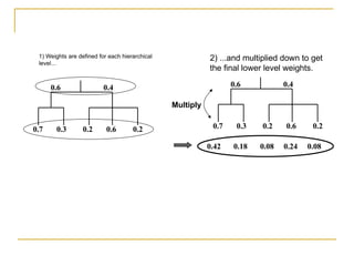
1) Weights aredefined for each hierarchical
level...
2) ...and multiplied down to get
the final lower level weights.
0.6 0.4
0.7 0.3 0.2 0.6 0.2
0.6 0.4
0.7 0.3 0.2 0.6 0.2
Multiply
0.42 0.18 0.08 0.24 0.08
41.
Notes:
• In general,the evaluation scores are collected from
many experts and the average scores is used in the
pairwise comparison matrix.
•The AHP solving is computer-aided by Expert Choice
(EC) software.
- Building structure of problem !!!
- Enter judgments (Pairwise Comparisons)
- Analysis the weights
- Sensitivity Analysis
- Advantages and disadvantages
- Miscellaneous
42.
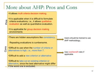
More about AHP:Pros and Cons
42
•There are hidden assumptions like consistency.
Repeating evaluations is cumbersome.
•Difficult to use when the number of criteria or
alternatives is high, i.e., more than 7.
•Difficult to add a new criterion or alternative
•Difficult to take out an existing criterion or
alternative, since the best alternative might differ
if the worst one is excluded.
Users should be trained to use
AHP methodology.
Use cost/benefit ratio if
applicable
Pros
Cons
•It allows multi criteria decision making.
•It is applicable when it is difficult to formulate
criteria evaluations, i.e., it allows qualitative
evaluation as well as quantitative evaluation.
•It is applicable for group decision making
environments
#4 Example: Buying a computer or laptop, smart phone: have to consider some factor: cost, brand name, specifications, …
Give the weights for each of these factor (cost 60%, specification 30% and brand name 10%)
Give the scores of each factor for the alternatives you want to buy.
#9 In many situations one may not be able to assign weights to the different decision factors. Therefore one must rely on a technique that will allow the estimation of the weights.
What is a solution?
One such process, The Analytical Hierarchy Process (AHP), involves pairwise comparisons between the various factors.
Method for ranking decision alternatives and selecting the best one when the decision maker has multiple objectives, or criteria
#13 A compare with A = 1
consider the apple A and B about the size. A = 2B => B= ½A
Explain Eigenvector later
#14 If compare through verbal judgment, the judgments will be transform to numerical values.
#15 In this example, Cost is not a factor. It will be consider later.
#18 Normalize is to transform the values to proportion (sum will be 1)
#22 Prof. Saaty suggest the compare CI with the Random Consistency Index RI
#24 Similar with Factor Ranking, the Priority vectors of Alternatives are determined.
The corresponding CR should be determined to ensure the consistency of pair-wise judgment


![18
Ranking of Priorities
Consider [Ax = x] where
A is the comparison matrix of size n×n, for n criteria, also called the priority
matrix.
x is the Eigenvector of size n×1, also called the priority vector.
is the Eigenvalue, > n.
To find the ranking of priorities, namely the Eigen Vector X:
1) Normalize the column entries by dividing each entry by the sum of the column.
2) Take the overall row averages.
0.30 0.29 0.38
0.60 0.57 0.50
0.10 0.14 0.13
Column sums 3.33 1.75 8.00 1.00 1.00 1.00
A=
1 0.5 3
2 1 4
0.33 0.25 1.0
Normalized
Column Sums
Row
Averages
0.3196
0.5584
0.1220
Priority vector
X=
Example 1: Car Selection (4/15)
Example 1: Car Selection (4/15)
Pairwise Comp. Matrix Norm. Pairwise Comp. Matrix](https://image.slidesharecdn.com/ahpvf-250602113342-77596718/85/Introduction-to-AHP-Method-Examples-and-Introduction-18-320.jpg)
![21
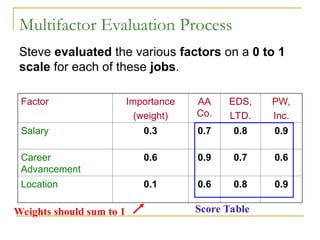
Calculation of Consistency Ratio
0.30
0.60
0.10
1 0.5 3
2 1 4
0.333 0.25 1.0
0.90
1.60
0.35
=
A x Ax x
=
A x Ax x
Consistency index (CI) is found by
The next stage is to calculate , Consistency Index (CI) and the
Consistency Ratio (CR).
Consider [Ax = x] where x is the Eigenvector.
= =
0.30
0.60
0.10
A x Ax x
Example 1: Car Selection (7/15)
Consistency Vector =
0.90/0.30
1.60/0.60
0.35/0.10
06
.
3
3
5
.
3
67
.
2
0
.
3
3.00
2.67
3.50
=
03
.
0
1
3
3
06
.
3
1
n
n
CI
Note: This is just an approximate method to determine value of λ](https://image.slidesharecdn.com/ahpvf-250602113342-77596718/85/Introduction-to-AHP-Method-Examples-and-Introduction-21-320.jpg)