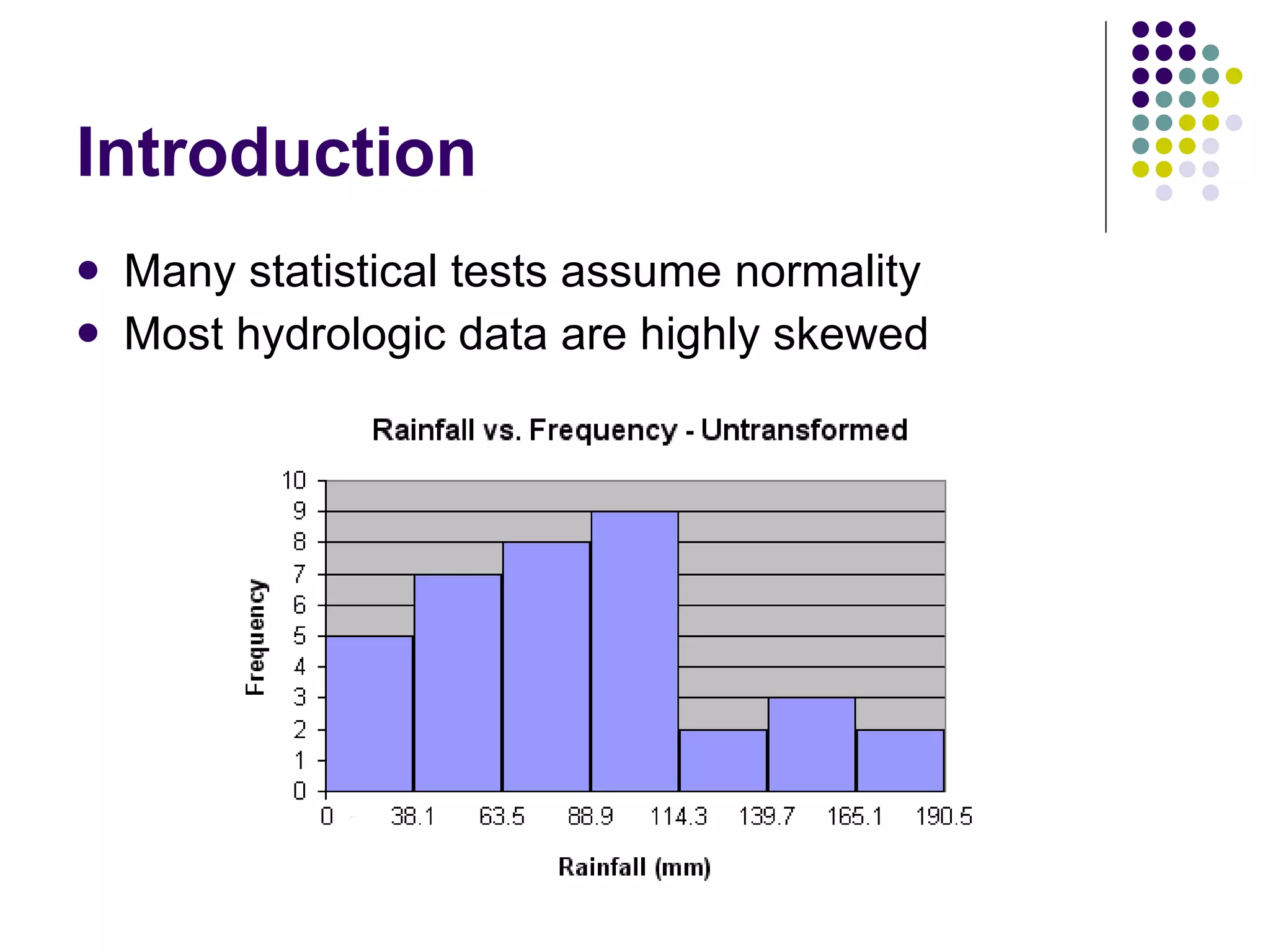
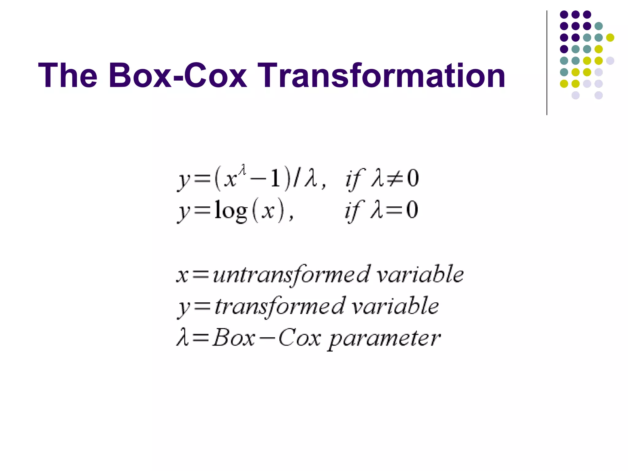
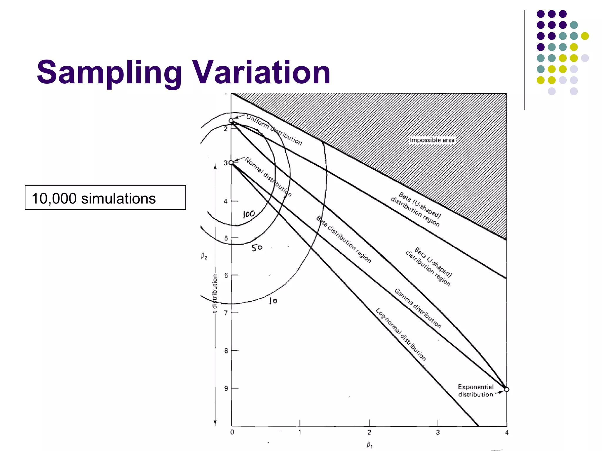
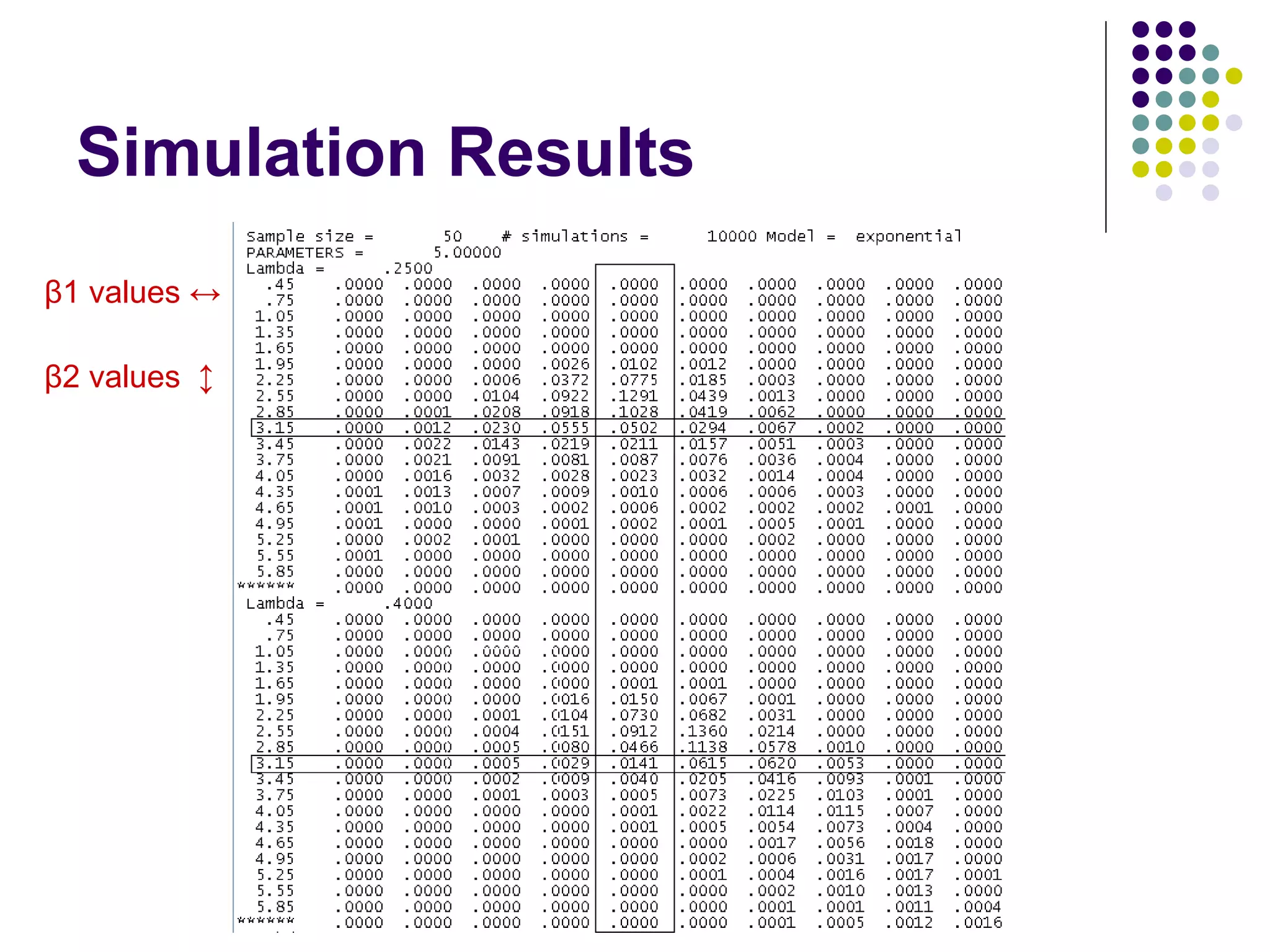
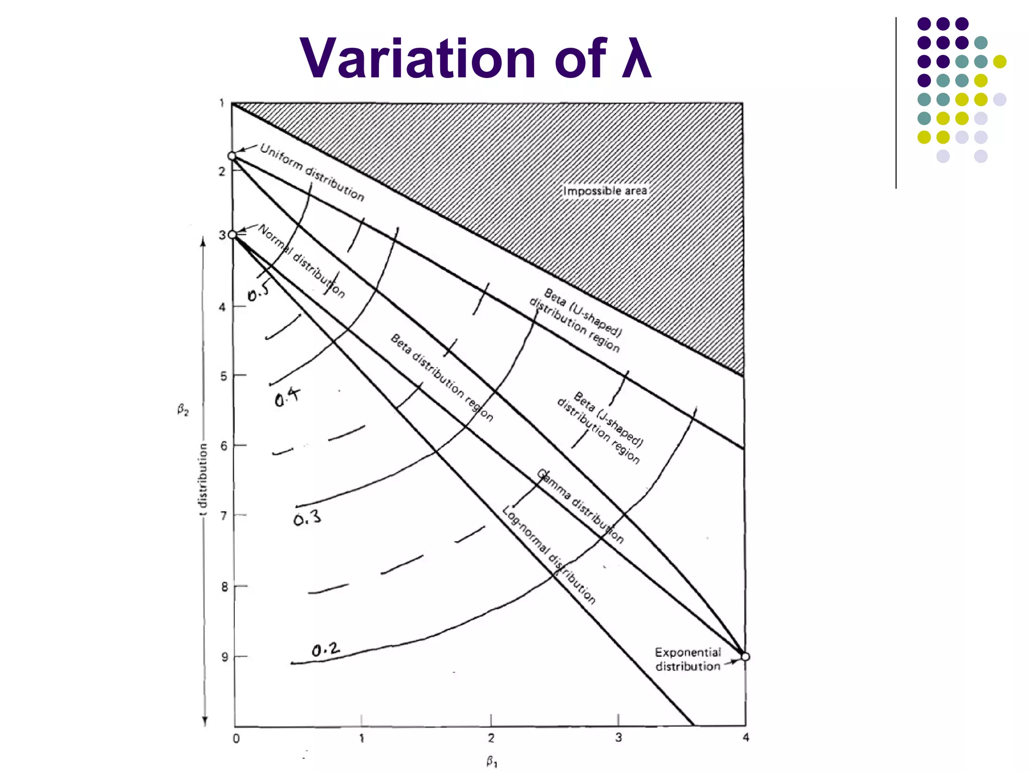
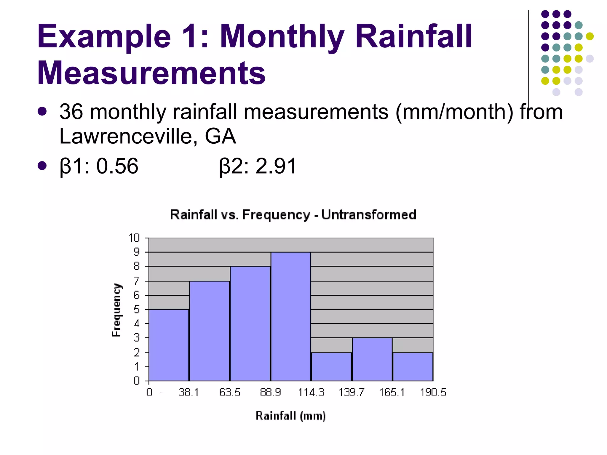
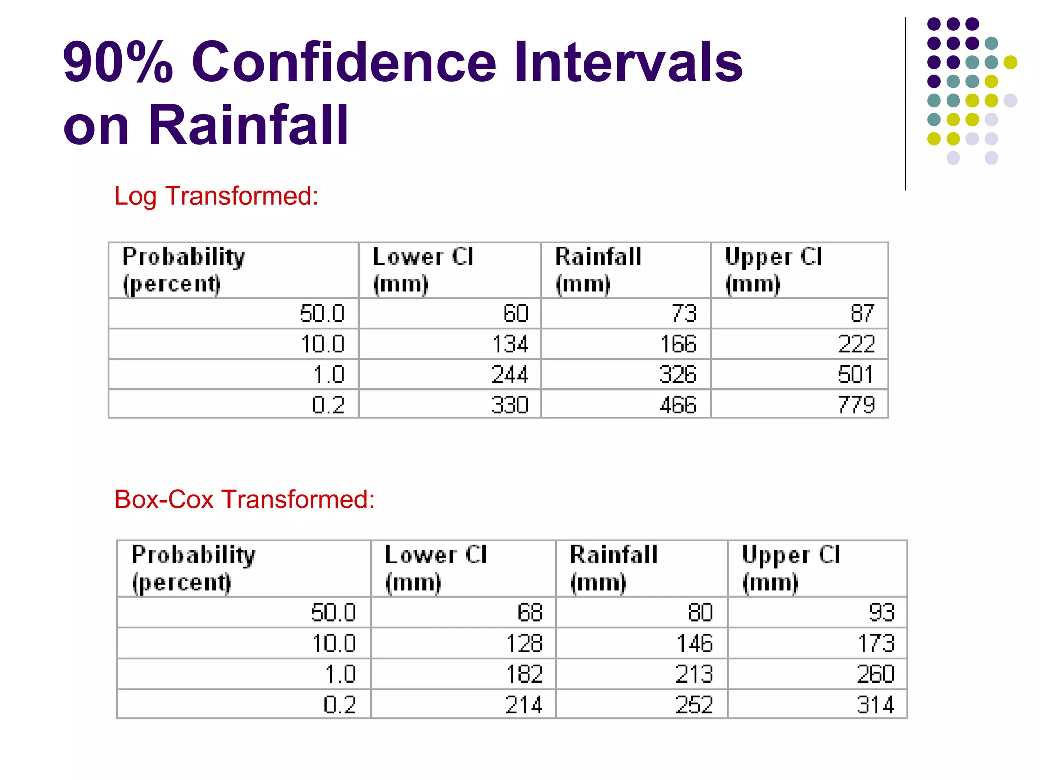
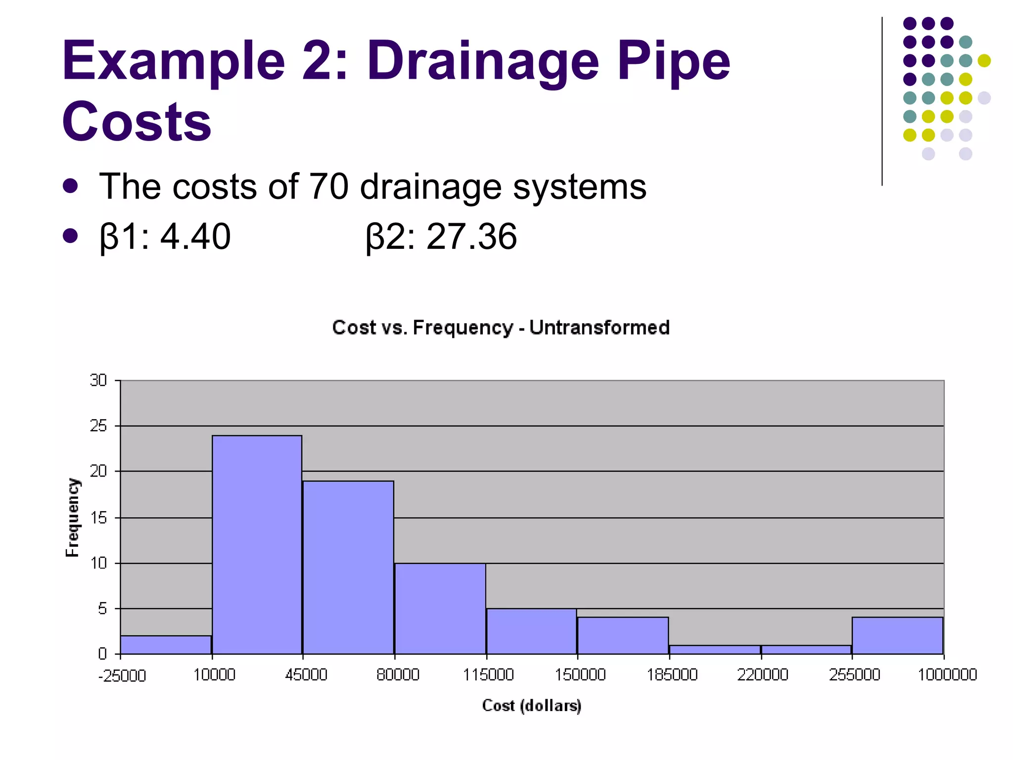
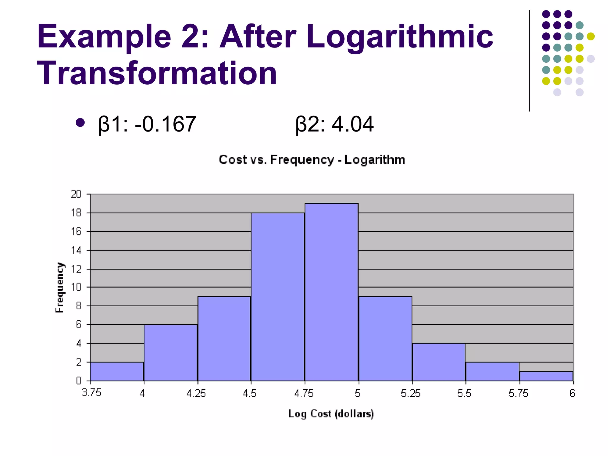
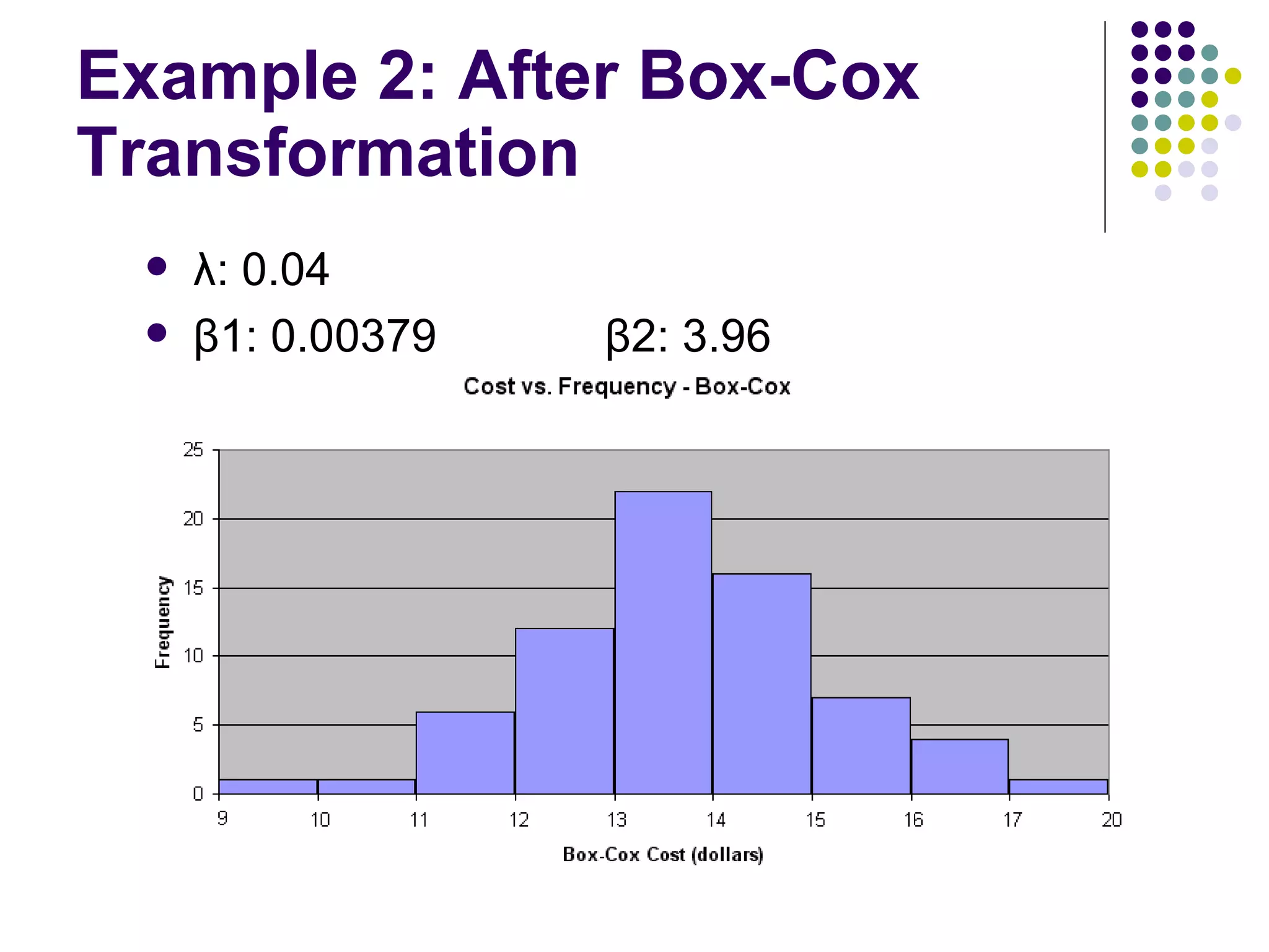
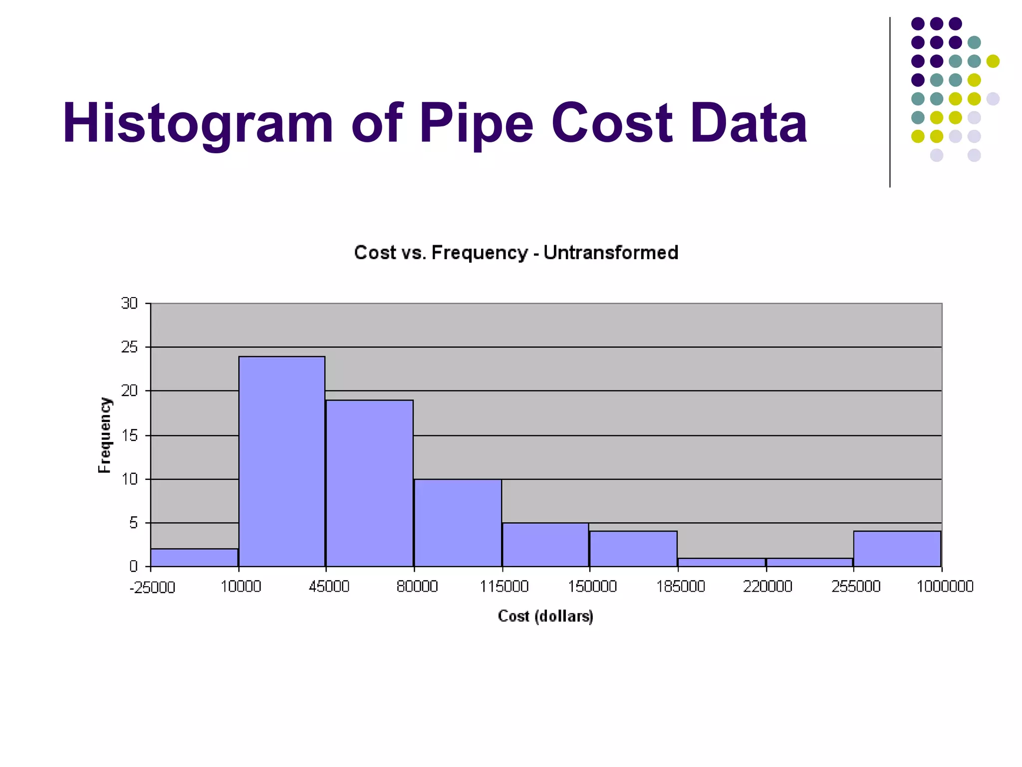
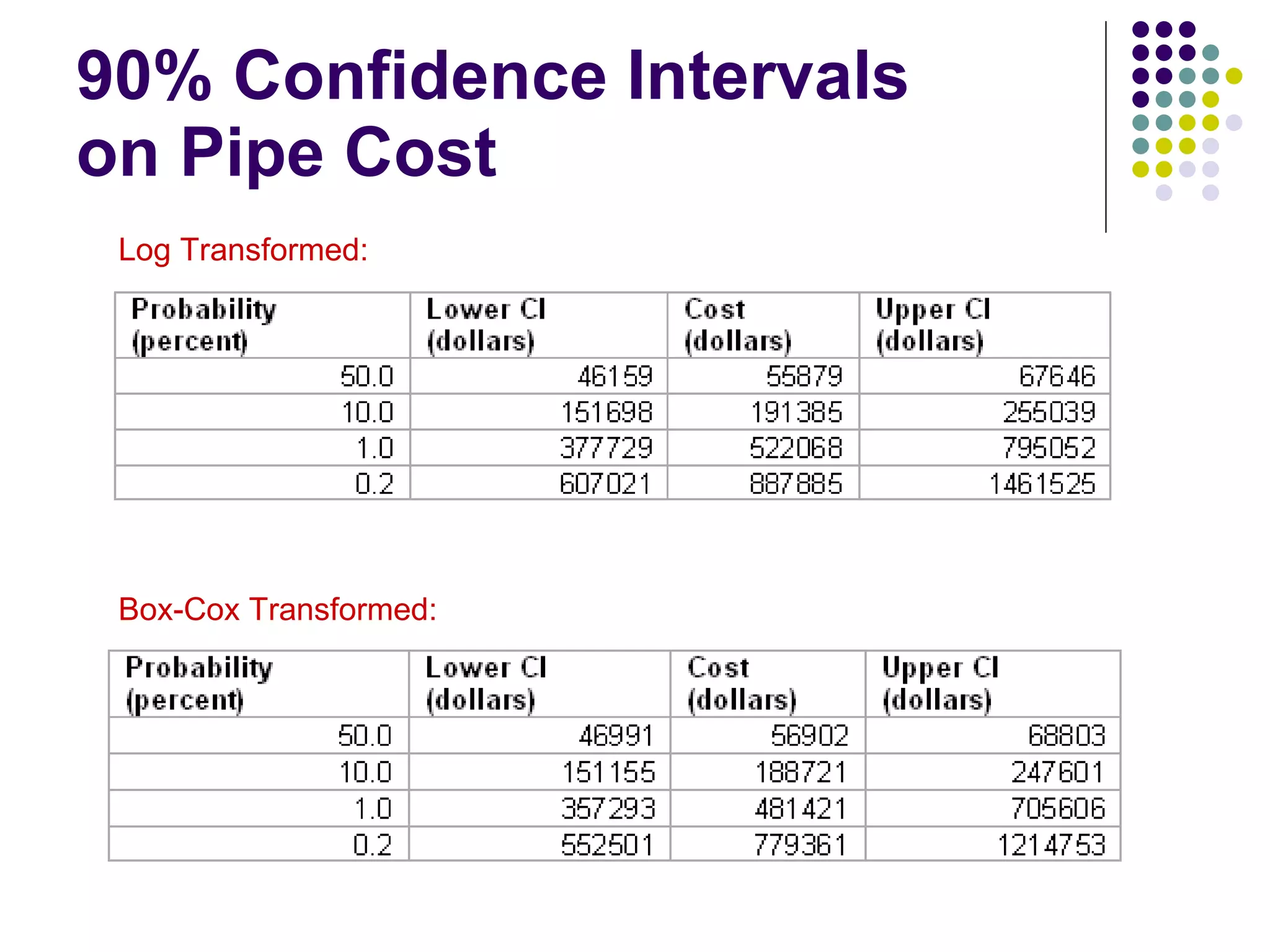
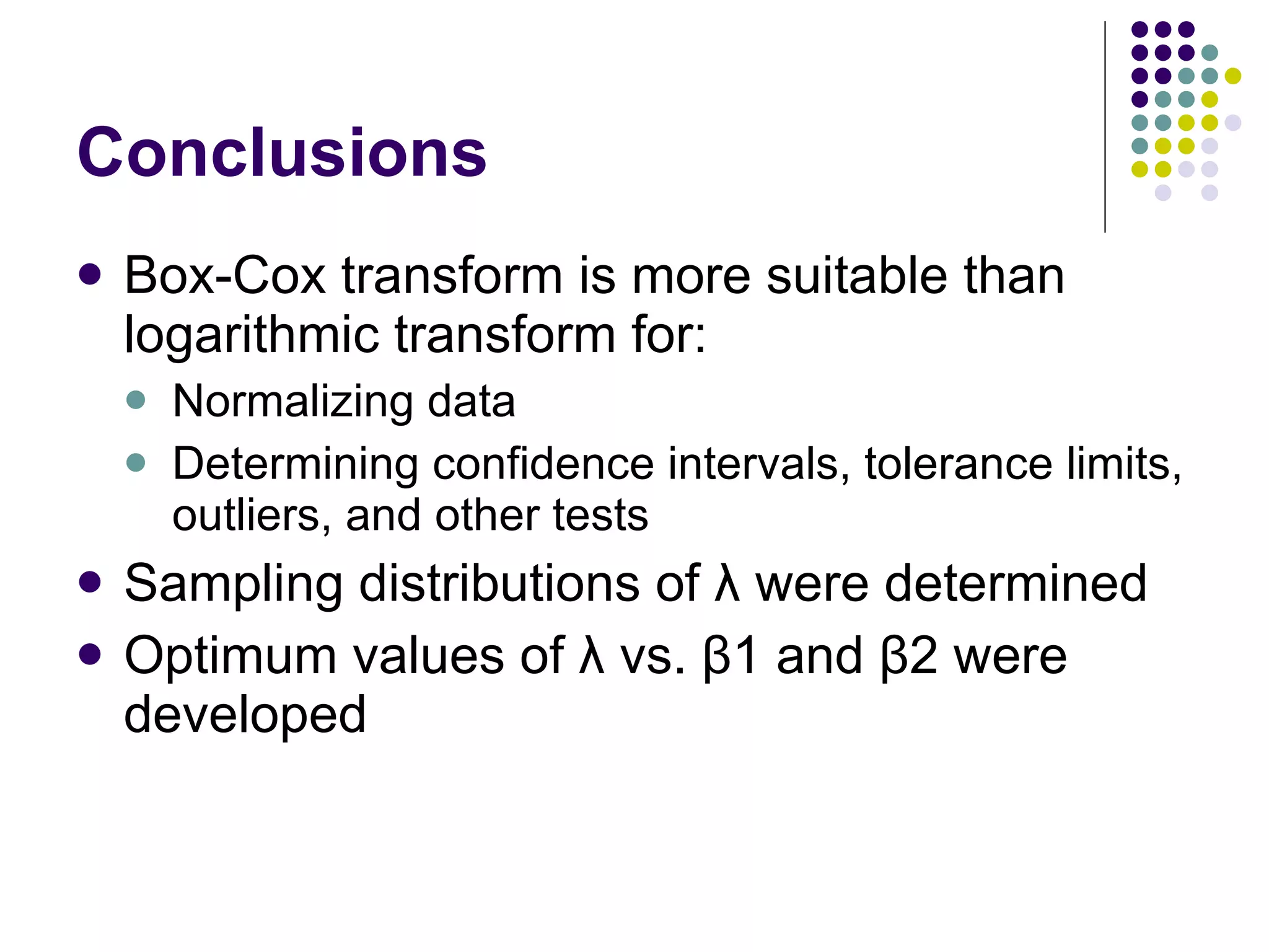
Estimation of the Box-Cox Transformation Parameter and Application to Hydrologic Data Melanie Wong Friday, August 29, 2008
Introduction Many statistical tests assume normality Most hydrologic data are highly skewed
Detecting Normality β1 (third moment) = skewness β2 (fourth moment) = kurtosis Characteristics of a normal distribution: β1=0 β2=3
Moment Ratio Diagram
Transformation to Normality Hydrologic data are not normal Various transformations available Logarithmic Box-Cox
The Box-Cox Transformation
Transformation Procedure Decide if sample data is normal Obtain value of λ Transform the data Apply confidence intervals, statistical  tests, or tolerance limits Perform inverse transformation
Determining the Optimal λ “ Snap-to-the-grid” method Box and Cox (1967): “... fix one, or possibly a small number, of λ's and go ahead with the detailed estimation...” Distribution-based method λ=-1.0 reciprocal transform λ=-0.5 reciprocal square root transform λ=0  natural log transform λ=+0.5 square root transform λ=1.0 no transformation needed
Research Goal and Objectives Goal: To develop a better understanding of the Box-Cox transformation so that it can be applied with greater confidence Objectives: To characterize the sampling variation To provide a method for estimating the Box-Cox transformation parameter for any set of data
Sampling Variation 10,000 simulations
Second Objective To provide a method for estimating the Box-Cox transformation parameter  for any set of data
The Importance of λ Small changes in λ    Large  changes in sampling variation Need a more precise method  to obtain optimum λ
Optimizing λ Procedure: Monte Carlo simulation to identify sampling distributions of β1 and β2 values for different λ values Distribution types: Gamma, exponential, uniform Population sizes: 1000, 500, 200, 100, 50, 10
Simulation Results β1 values  ↔ β2 values  ↕
Variation of λ
Confidence Intervals Procedure: Logarithmic 1) Make Logarithmic transformation of x 2) Use normal theory for confidence intervals on y 3) Inverse transform the confidence intervals  to values of x
Confidence Interval Procedure: Box-Cox 1) Make BCT of x to y using optimum λ 2) Use normal theory for confidence intervals on y 3) Inverse transform the confidence intervals to  values of x
Example 1: Monthly Rainfall Measurements 36 monthly rainfall measurements (mm/month) from Lawrenceville, GA β1: 0.56 β2: 2.91
Example 1: After Logarithmic Transformation β1: -1.12 β2: 4.40
Example 1: After Box-Cox Transformation λ: 0.55 β1: -0.09 β2: 2.82
Histogram of Rainfall Data
90% Confidence Intervals  on Rainfall Box-Cox Transformed: Log Transformed:
Example 2: Drainage Pipe Costs The costs of 70 drainage systems β1: 4.40  β2: 27.36
Example 2: After Logarithmic Transformation β1: -0.167 β2: 4.04
Example 2: After Box-Cox Transformation λ: 0.04 β1: 0.00379 β2: 3.96
Histogram of Pipe Cost Data
90% Confidence Intervals  on Pipe Cost Box-Cox Transformed: Log Transformed:
Conclusions Box-Cox transform is more suitable than logarithmic transform for: Normalizing data Determining confidence intervals, tolerance limits, outliers, and other tests Sampling distributions of λ were determined Optimum values of λ vs. β1 and β2 were developed
QUESTIONS?

Estimation Of The Box Cox Transformation Parameter And Application To Hydrologic Data 1

  • 1.
    Estimation of theBox-Cox Transformation Parameter and Application to Hydrologic Data Melanie Wong Friday, August 29, 2008
  • 2.
    Introduction Many statisticaltests assume normality Most hydrologic data are highly skewed
  • 3.
    Detecting Normality β1(third moment) = skewness β2 (fourth moment) = kurtosis Characteristics of a normal distribution: β1=0 β2=3
  • 4.
  • 5.
    Transformation to NormalityHydrologic data are not normal Various transformations available Logarithmic Box-Cox
  • 6.
  • 7.
    Transformation Procedure Decideif sample data is normal Obtain value of λ Transform the data Apply confidence intervals, statistical tests, or tolerance limits Perform inverse transformation
  • 8.
    Determining the Optimalλ “ Snap-to-the-grid” method Box and Cox (1967): “... fix one, or possibly a small number, of λ's and go ahead with the detailed estimation...” Distribution-based method λ=-1.0 reciprocal transform λ=-0.5 reciprocal square root transform λ=0 natural log transform λ=+0.5 square root transform λ=1.0 no transformation needed
  • 9.
    Research Goal andObjectives Goal: To develop a better understanding of the Box-Cox transformation so that it can be applied with greater confidence Objectives: To characterize the sampling variation To provide a method for estimating the Box-Cox transformation parameter for any set of data
  • 10.
  • 11.
    Second Objective Toprovide a method for estimating the Box-Cox transformation parameter for any set of data
  • 12.
    The Importance ofλ Small changes in λ  Large changes in sampling variation Need a more precise method to obtain optimum λ
  • 13.
    Optimizing λ Procedure:Monte Carlo simulation to identify sampling distributions of β1 and β2 values for different λ values Distribution types: Gamma, exponential, uniform Population sizes: 1000, 500, 200, 100, 50, 10
  • 14.
    Simulation Results β1values ↔ β2 values ↕
  • 15.
  • 16.
    Confidence Intervals Procedure:Logarithmic 1) Make Logarithmic transformation of x 2) Use normal theory for confidence intervals on y 3) Inverse transform the confidence intervals to values of x
  • 17.
    Confidence Interval Procedure:Box-Cox 1) Make BCT of x to y using optimum λ 2) Use normal theory for confidence intervals on y 3) Inverse transform the confidence intervals to values of x
  • 18.
    Example 1: MonthlyRainfall Measurements 36 monthly rainfall measurements (mm/month) from Lawrenceville, GA β1: 0.56 β2: 2.91
  • 19.
    Example 1: AfterLogarithmic Transformation β1: -1.12 β2: 4.40
  • 20.
    Example 1: AfterBox-Cox Transformation λ: 0.55 β1: -0.09 β2: 2.82
  • 21.
  • 22.
    90% Confidence Intervals on Rainfall Box-Cox Transformed: Log Transformed:
  • 23.
    Example 2: DrainagePipe Costs The costs of 70 drainage systems β1: 4.40 β2: 27.36
  • 24.
    Example 2: AfterLogarithmic Transformation β1: -0.167 β2: 4.04
  • 25.
    Example 2: AfterBox-Cox Transformation λ: 0.04 β1: 0.00379 β2: 3.96
  • 26.
  • 27.
    90% Confidence Intervals on Pipe Cost Box-Cox Transformed: Log Transformed:
  • 28.
    Conclusions Box-Cox transformis more suitable than logarithmic transform for: Normalizing data Determining confidence intervals, tolerance limits, outliers, and other tests Sampling distributions of λ were determined Optimum values of λ vs. β1 and β2 were developed
  • 29.