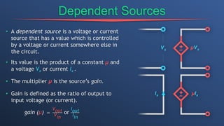
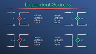
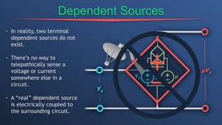
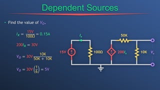
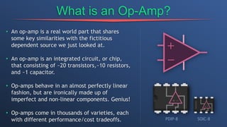
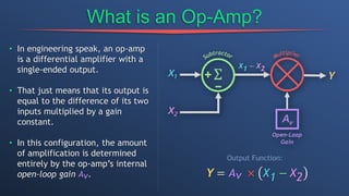
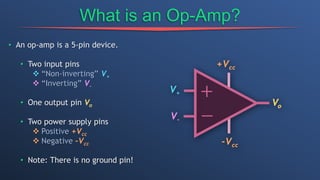
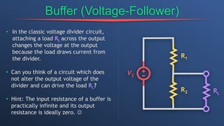
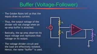
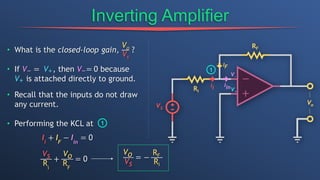
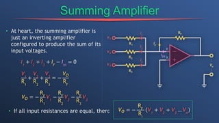
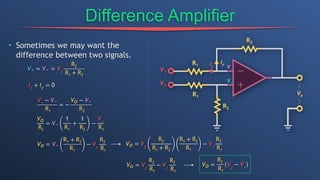
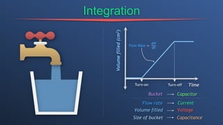
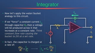
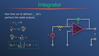
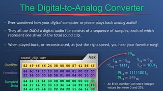
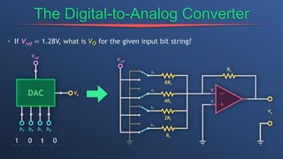
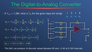
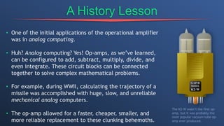
This document discusses dependent sources and operational amplifiers. It defines dependent sources as voltage or current sources whose value is controlled by another voltage or current in the circuit. Their value is the product of a constant gain and the controlling voltage or current. The document then discusses various op-amp configurations like inverting amplifiers, non-inverting amplifiers, summing amplifiers, and integrators. It explains how feedback is used to stabilize the op-amp and achieve a desired gain. The document also provides an overview of digital to analog converters and how they reconstruct analog waveforms from digital samples.

1. By Solid State Workshop
Essential & Practical
Circuit Analysis
Part 2: Op-Amps

2. Dependent Sources
• A dependent source is a voltage or current
source that has a value which is controlled
by a voltage or current somewhere else in
the circuit.
• Its value is the product of a constant μ and
a voltage Vx or current Ix .
• The multiplier μ is the source’s gain.
• Gain is defined as the ratio of output to
input voltage (or current).
gain (μ) =
Vout
Vin
or
Iout
Iin

3. Dependent Sources
Voltage
Controlled
Voltage
Source
Voltage
Controlled
Current
Source
Current
Controlled
Current
Source
Current
Controlled
Voltage
Source

4. Dependent Sources
• In reality, two terminal
dependent sources do not
exist.
• There’s no way to
telepathically sense a
voltage or current
somewhere else in a
circuit.
• A “real” dependent source
is electrically coupled to
the surrounding circuit.

5. Dependent Sources
• Find the value of Vo.
Ix =
15V
100Ω
= 0.15A
200Ix = 30V
Vo = 30V
10K
50K + 10K
Vo = 30V
1
6
= 5V

6. What is an Op-Amp?
• An op-amp is a real world part that shares
some key similarities with the fictitious
dependent source we just looked at.
• An op-amp is an integrated circuit, or chip,
that consisting of ~20 transistors,~10 resistors,
and ~1 capacitor.
• Op-amps behave in an almost perfectly linear
fashion, but are ironically made up of
imperfect and non-linear components. Genius!
• Op-amps come in thousands of varieties, each
with different performance/cost tradeoffs. SOIC-8
PDIP-8
+
−

7. What is an Op-Amp?
• In engineering speak, an op-amp
is a differential amplifier with a
single-ended output.
• That just means that its output is
equal to the difference of its two
inputs multiplied by a gain
constant.
• In this configuration, the amount
of amplification is determined
entirely by the op-amp’s internal
open-loop gain Av. Y = Av × X1 − X2
Output Function:

8. What is an Op-Amp?
• An op-amp is a 5-pin device.
• Two input pins
 “Non-inverting” V+
 “Inverting” V-
• One output pin Vo
• Two power supply pins
 Positive +Vcc
 Negative –Vcc
• Note: There is no ground pin!

9. Op-Amp Transfer Characteristics
• In the linear region…
Vo = AV (V+ – V−)
• In the saturation regions…
Vo = −Vcc or +Vcc

10. Taming the Gain
• Op-amps have huge values of Av, their open-
loop gains. (Between 105 and 108 typically)
• A differential input voltage of just 50mV would
send the output on its way to 5kV or more!
Note: It would hit the upper power supply
limit long before it got anywhere near 5kV.
• We need to “tame” the op-amp so that the
output isn’t so sensitive.
• That is, we need to reduce the effective gain.

11. We need feedback!
• It is impossible to reduce the open-loop gain of an op-
amp because it is internal to the op-amp.
• However, we can employ an external mechanism that
keeps the difference between the inputs so small that the
output stays within a practical range.
For ex. If V+ − V− = 25μV and AV = 100,000
Then, Vo = 2.5V 
• This mechanism is called negative feedback, in which
portion of the output signal is fed back to the input.
• β is the feedback factor which determines how much of
the output is fed back to the input. (0 < β ≤ 1)

12. How Does Feedback Work?
• This op-amp system is governed
by two simultaneous equations:
1. Vo = AV ∙ VΔ
V− = β ∙ Vo
V𝜟 = V+ − β ∙ Vo
2. Vo =
V+− VΔ
β
• Let’s solve it graphically 

13. Real Op-Amps vs. Ideal Op-Amps
• A real op-amp circuit (with feedback) works by maintaining a tiny voltage VΔ
between its inputs to counteract the op-amps huge internal gain AV.
• The op-amp regulates its own VΔ by adjusting its output voltage Vo which is
connected back to one of the inputs through a feedback network defined by β.
• We noticed that as AV was increased, the input differential voltage VΔ moved
closer to zero and the output voltage closer to the “target”.
• That is, the op-amp approached ideal operation.
• Classic op-amp circuit analysis always assumes ideal operation in favor of
simplicity. However, today’s free SPICE software can paint a more accurate
picture of how an op-amp circuit works by accounting for real characteristics.

14. Ideal Op-Amp Characteristics
• An ideal op-amp has:
 Infinite open-loop gain
Av = ∞
 Infinite input resistance
Ri = ∞
 Zero output resistance
Ro = 0

15. Ideal Op-Amp Characteristics
• We are interested in amplification, so
we want to operate in the linear
region.
• However, if AV is infinite, then the
only way to stay in the linear region is
if (V+ − V-) is equal to 0.
• That is, V+ must be equal to V-.
 Infinite open-loop gain
Av = ∞
Vo = AV (V+ – V−)

16. • An amplifier should be “invisible” to
whatever sources are connected to
its inputs.
• An ideal op-amp has infinite input
resistance so no current flows into
the op-amp’s inputs.
• Thus, I+ and I- must both be 0.
Ideal Op-Amp Characteristics
 Infinite input resistance
Ri = ∞

17. The Golden Rules
• Based on what we just learned, let’s
formally state the two “Golden Rules” of
op-amps.
 I. The output attempts to do whatever
is necessary to make the voltage
difference between the inputs zero.
 II. The inputs draw no current.
• With these two rules, we are now ready to
solve any ideal op-amp circuit.
Credit: “The Art of Electronics” (3rd) by Horowitz and Hill

18. Non-Inverting Amplifier
• What is the closed-loop gain,
Vo
Vs
?
• Since V+ = Vs , the op-amp must
“do whatever it takes” to make
V- = V+ = Vs .
• Now, notice that V- is the output
voltage of a voltage divider
consisting of RF and RG.
• Remember that a voltage divider
produces a voltage which is a
fraction (β) of its input voltage.
β

19. Non-Inverting Amplifier
β
• The only way the output of the
divider V− can equal Vs is if the
input to the divider Vo is a
voltage larger than Vs.
• That’s amplification!
V− = V+ = Vs
V− = Vs = Vo ×
RG
RG + RF
Vo
Vs
=
RG + RF
RG
β
Vo
Vs
=1 +
RF
RG

20. Buffer (Voltage-Follower)
• The buffer is really just a non-
inverting amplifier without a
feedback resistor network.
• In order to keep V− = V+, the op-
amp must produce a voltage Vo
which is exactly equal to Vs .
• That is, its gain, Vo
Vs
, is 1.
• So, what’s the point?

21. Buffer (Voltage-Follower)
RL
VS
R1
R2
• In the classic voltage divider circuit,
attaching a load RL across the output
changes the voltage at the output
because the load draws current from
the divider.
• Can you think of a circuit which does
not alter the output voltage of the
divider and can drive the load RL?
• Hint: The input resistance of a buffer is
practically infinite and its output
resistance is ideally zero. 

22. Buffer (Voltage-Follower)
• The Golden Rules tell us that the
inputs draw no current.
• Thus, the output voltage of the
divider will not change when an
op-amp buffer is attached.
• Basically, the op-amp observes its
input voltage and replicates that
voltage on its output.
• The voltage divider circuit and
the load are effectively isolated.
Hence, the name “buffer” is used.

23. Inverting Amplifier
• What is the closed-loop gain,
Vo
Vs
?
• If V− = V+, then V−= 0 because
V+ is attached directly to ground.
• Recall that the inputs do not draw
any current.
• Performing the KCL at
1
1
Ii
IF
Iin
Ii
+ IF
− Iin
= 0
Vs
Ri
+
Vo
RF
= 0
Vo
Vs
= −
RF
Ri

24. Summing Amplifier
• At heart, the summing amplifier is
just an inverting amplifier
configured to produce the sum of its
input voltages.
I1
+ I2
+ I3
+ IF
− Iin
= 0
I1
I2
I3
IF
Iin
V1
R1
+
V2
R2
+
V3
R3
= −
Vo
RF
Vo = −
RF
R1
V1
−
RF
R2
V2
−
RF
R3
V3
• If all input resistances are equal, then: Vo = −
RF
Ri
V1
+ V2
+ V3
… Vn

25. Difference Amplifier
• Sometimes we may want the
difference between two signals.
V+ = V− = V2
R2
R1 + R2
I1
+ IF
= 0
I1
IF
V1
− V−
R1
= −
Vo − V−
R2
Vo
R2
= V−
1
R1
+
1
R2
−
V1
R1
Vo = V−
R1 + R2
R1
− V1
R2
R1
Vo = V2
R2
R1
− V1
R2
R1
Vo =
R2
R1
V2
− V1
Vo = V2
R2
R1 + R2
R1 + R2
R1
− V1
R2
R1

26. Integration
Flow Rate =
dV
dt
Volume
filled
(cm
3
)
Time
Turn-on Turn-off
Volume filled Voltage
Flow rate Current
Capacitor
Bucket
Size of bucket Capacitance

27. Integrator
• Now let’s apply the water/bucket
analogy to this circuit.
• If we “force” a constant current ICF
through capacitor CF then a voltage
will be produced across it that
increases at a constant rate. Think
constant flow rate causing the
bucket to fill at a set rate.
• In fact, the capacitor is charged at
a rate of:
ICF
ICF
= CF
dVo
dt
dVo
dt
=
ICF
CF

28. Integrator
• Now that we’ve defined ICF
let’s
perform the nodal analysis.
Is
+ ICF
= 0
Vs
Ri
= −CF
dVo
dt
dVo
dt
= −
1
Ri
CF
Vs
Vo = −
1
Ri
CF
Vs dt + C
Is
ICF

29. The Digital-to-Analog Converter
• Ever wondered how your digital computer or phone plays back analog audio?
• They all use DACs! A digital audio file consists of a sequence of samples, each of which
represent one sliver of the total sound clip.
• When played back, or reconstructed, at just the right speed, you hear your favorite song!
f916
f16 = 1510
916 = 910
1510 = 11112 910 = 10012
f916 = 111110012
f916 = 24910
• An 8-bit number can store integer
values between 0 and 255.
52 49 46 46 24 08 00 00 57 41 56 45
66 6d 74 20 10 00 00 00 01 00 02 00
22 56 00 00 88 58 01 00 04 00 10 00
64 61 74 61 00 08 00 00 00 00 00 00
24 17 1e f3 3c 13 3c 14 16 f9 18 f9
34 e7 23 a6 3c f2 24 f2 11 ce 1a 0d
Sampled
Data
ChunkDesc
FormatDesc
Hex
sound_clip.wav

30. The Digital-to-Analog Converter
• If Vref = 1.28V, what is Vo for the given input bit string?

31. • If Vref = 1.28V, what is Vo for the given input bit string?
The Digital-to-Analog Converter
b0
b1
b2
b3
Vo = −Vref
Ri
Ri
b3 +
Ri
2Ri
b2 +
Ri
4Ri
b1 +
Ri
8Ri
b0
Vo = −Vref 1b3 +
1
2
b2 +
1
4
b1 +
1
8
b0
Vo = −1.28 1 1 +
1
2
0 +
1
4
1 + 0
Vo = −1.28 × 1.25 = −1.6V
• This DAC can produce 16 discrete values between 0V and −2.4V at 0.16V intervals.

32. A History Lesson
• One of the initial applications of the operational amplifier
was in analog computing.
• Huh? Analog computing? Yes! Op-amps, as we’ve learned,
can be configured to add, subtract, multiply, divide, and
even integrate. These circuit blocks can be connected
together to solve complex mathematical problems.
• For example, during WWII, calculating the trajectory of a
missile was accomplished with huge, slow, and unreliable
mechanical analog computers.
• The op-amp allowed for a faster, cheaper, smaller, and
more reliable replacement to these clunking behemoths.
The K2-W wasn’t the first op-
amp, but it was probably the
most popular vacuum tube op-
amp ever produced.

33. Modeling a Real World System
y′′(t) =
1
M
(x(t) − By′(t) − Ky(t))

34. Thanks for watching!
I’d love to hear your feedback!
Subscribe