Downloaded 72 times


![USING IMAGE ANALYSIS FOR ARCGIS70
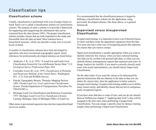
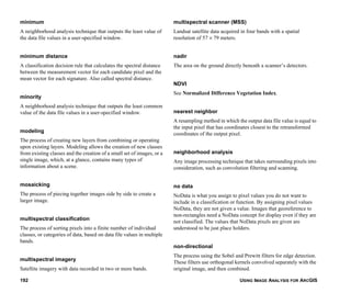
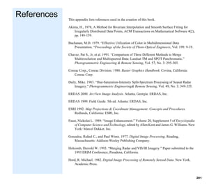
Convolution
Convolution filtering is the process of averaging small sets of pixels
across an image. Convolution filtering is used to change the spatial
frequency characteristics of an image (Jensen 1996).
A convolution kernel is a matrix of numbers that is used to average
the value of each pixel with the values of surrounding pixels. The
numbers in the matrix serve to weight this average toward
particular pixels. These numbers are often called coefficients,
because they are used as such in the mathematical equations.
Applying convolution filtering
Apply Convolution filtering by clicking the Image Analysis
dropdown arrow, and choosing Convolution from the Spatial
Enhancement menu. The word filtering is a broad term, which
refers to the altering of spatial or spectral features for image
enhancement (Jensen 1996). Convolution filtering is one method of
spatial filtering. Some texts use the terms synonymously.
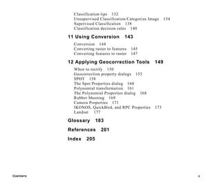
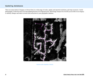
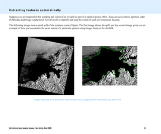
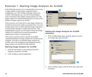
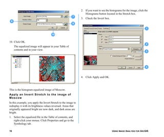
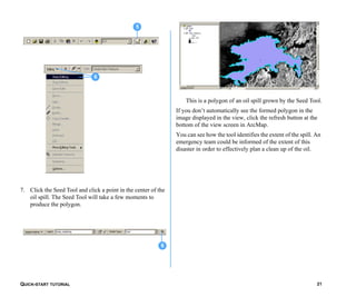
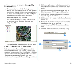
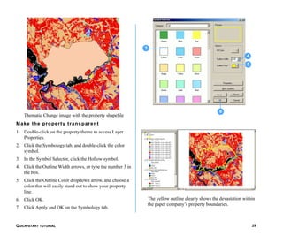
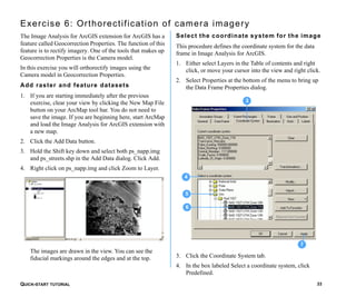
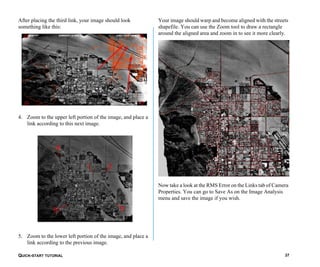
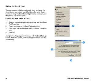
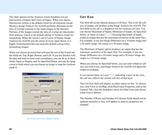
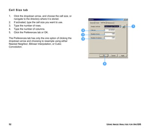
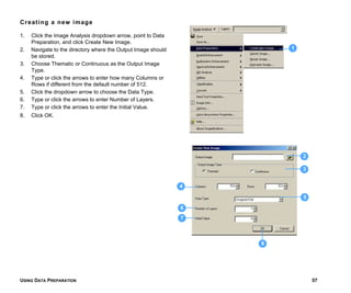
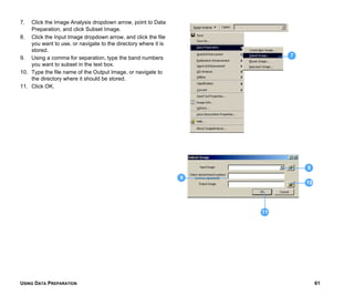
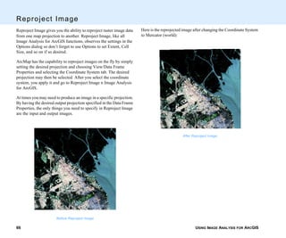
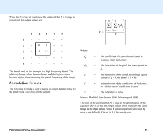
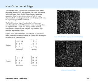
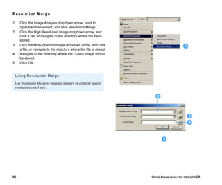
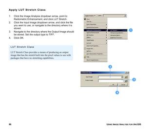
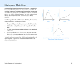
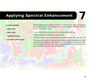
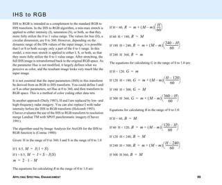
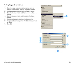
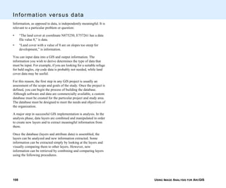
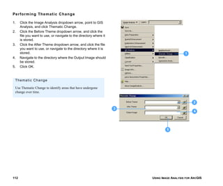
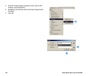
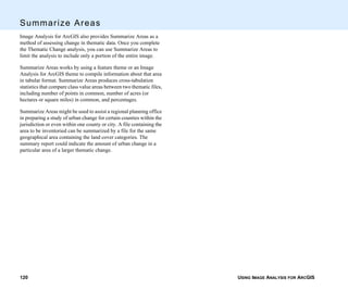
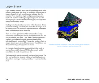
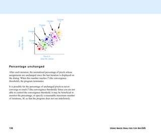
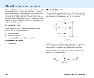
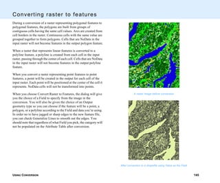
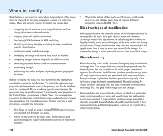
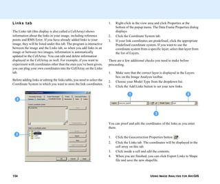
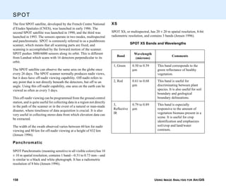
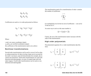
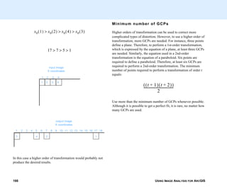
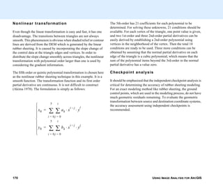
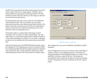
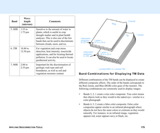
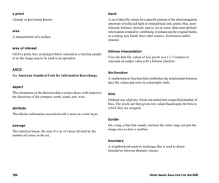
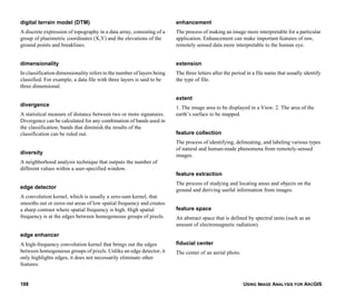
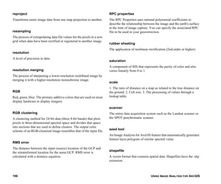
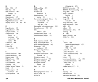
Convolution example
To understand how one pixel is convolved, imagine that the
convolution kernel is overlaid on the data file values of the image
(in one band) so that the pixel to be convolved is in the center of the
window. To compute the output value for this pixel, each value in the
convolution kernel is multiplied by the image pixel value that
corresponds to it. These products are summed, and the total is
divided by the sum of the values in the kernel, as shown in this
equation:
integer [((-1 × 8) + (-1 × 6) + (-1 × 6) +
(-1 × 2) + (16 × 8) + (-1 × 6) +
(-1 × 2) + (-1 × 2) + (-1 × 8))/
: (-1 + -1 + -1 + -1 + 16 + -1 + -1 + -1 + -1)]
= int [(128-40) / (16-8)]
= int (88 / 8) = int (11) = 11
2 8 6 6 6
2 8 6 6 6
2 2 8 6 6
2 2 2 8 6
2 2 2 2 8
Kernel
-1 -1 -1
-1 16 -1
-1 -1 -1
Data](https://image.slidesharecdn.com/erdas-imageanalysisforarcgis-160205132516/85/Erdas-image-analysis-for-arcgis-78-320.jpg)
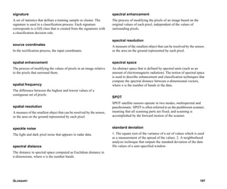
![PERFORMING SPATIAL ENHANCEMENT 79
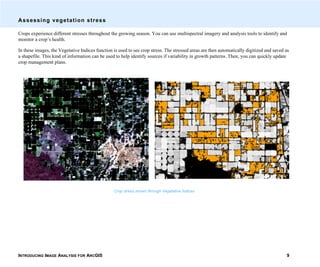
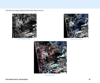
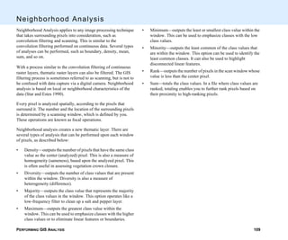
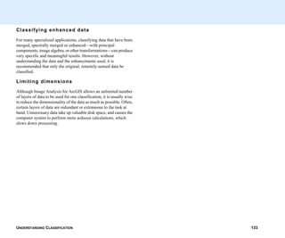
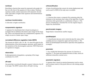
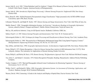
Resolution Merge
The resolution of a specific sensor can refer to radiometric, spatial,
spectral, or temporal resolution. This function merges imagery of
differing spatial resolutions.
Landsat TM sensors have seven bands with a spatial resolution of
28.5 m. SPOT panchromatic has one broad band with very good
spatial resolution—10 m. Combining these two images to yield a
seven-band data set with 10 m resolution provides the best
characteristics of both sensors.
A number of models have been suggested to achieve this image
merge. Welch and Ehlers (1987) used forward-reverse RGB to IHS
transforms, replacing I (from transformed TM data) with the SPOT
panchromatic image. However, this technique is limited to three
bands (R,G,B).
Chavez (1991), among others, uses the forward-reverse principal
components transforms with the SPOT image, replacing PC-1.
In the above two techniques, it is assumed that the intensity
component (PC-1 or I) is spectrally equivalent to the SPOT
panchromatic image, and that all the spectral information is
contained in the other PCs or in H and S. Since SPOT data does not
cover the full spectral range that TM data does, this assumption
does not strictly hold. It is unacceptable to resample the thermal
band (TM6) based on the visible (SPOT panchromatic) image.
Another technique (Schowengerdt 1980) additively combines a
high frequency image derived from the high spatial resolution data
(i.e., SPOT panchromatic) with the high spectral resolution Landsat
TM image.
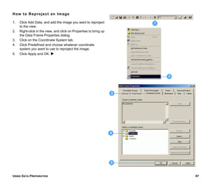
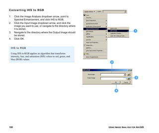
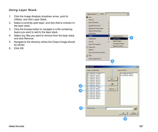
The Resolution Merge function uses the Brovey Transform method
of resampling low spatial resolution data to a higher spatial
resolution while retaining spectral information:
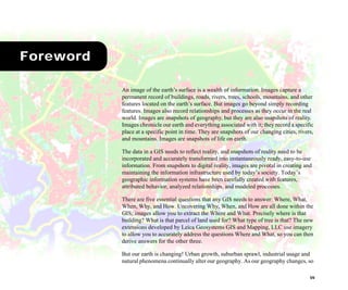
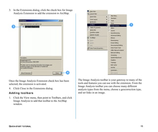
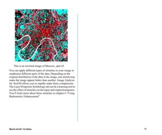
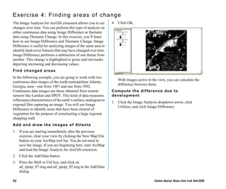
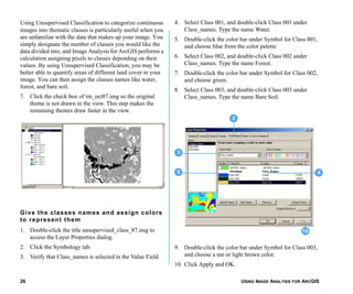
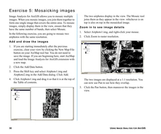
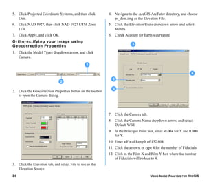
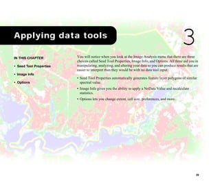
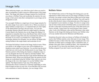
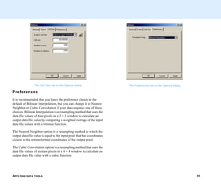
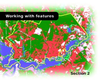
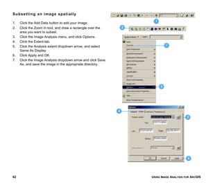
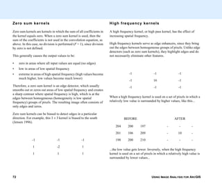
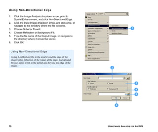
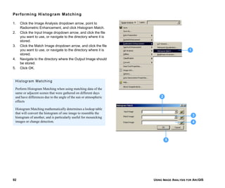
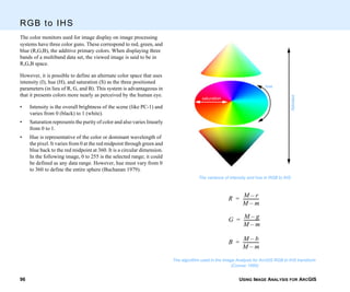
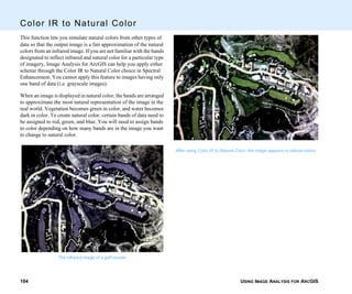
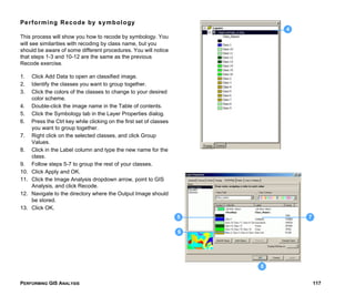
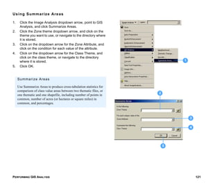
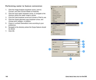
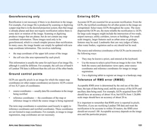
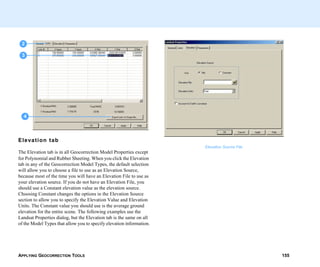
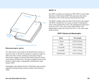
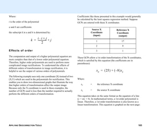
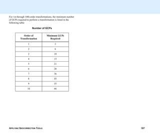
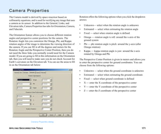
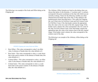
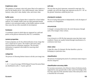
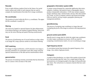
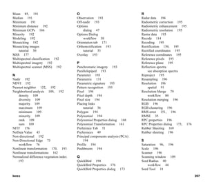
Brovey Transform
In the Brovey Transform, three bands are used according to the
following formula:
DNB1_new = [DNB1 / DNB1 + DNB2 + DNB3] ×
[DNhigh res. image]
DNB2_new = [DNB2 / DNB1 + DNB2 + DNB3] ×
[DNhigh res. image]
DNB3_new = [DNB3 / DNB1 + DNB2 + DNB3] ×
[DNhigh res. image]
Where:
B = band
The Brovey Transform was developed to visually increase contrast
in the low and high ends of an image’s histogram (i.e., to provide
contrast in shadows, water and high reflectance areas such as urban
features). Brovey Transform is good for producing RGB images
with a higher degree of contrast in the low and high ends of the
image histogram and for producing visually appealing images.
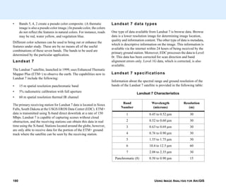
Since the Brovey Transform is intended to produce RGB images,
only three bands at a time should be merged from the input
multispectral scene, such as bands 3, 2, 1 from a SPOT or Landsat
TM image or 4, 3, 2 from a Landsat TM image. The resulting
merged image should then be displayed with bands 1, 2, 3 to RGB.](https://image.slidesharecdn.com/erdas-imageanalysisforarcgis-160205132516/85/Erdas-image-analysis-for-arcgis-87-320.jpg)


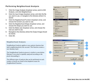


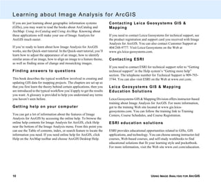
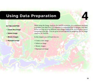
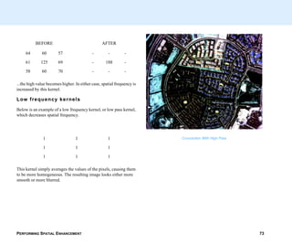
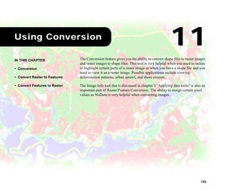
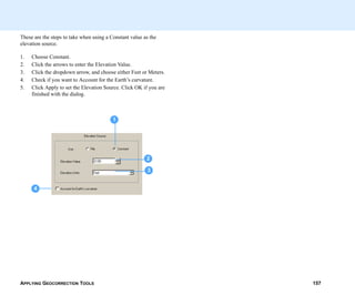
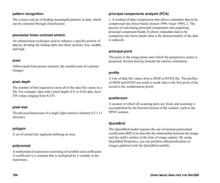
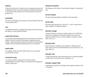
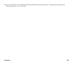
![UNDERSTANDING CLASSIFICATION 141
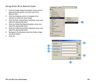
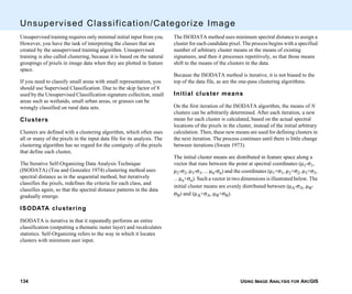
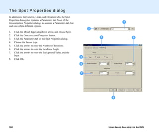
Where:
n = number of bands (dimensions)
i = a particular band
c = a particular class
Xxyi = data file value of pixel x,y in band i
µci = mean of data file values in band i for the
sample for class c
SDxyc = spectral distance from pixel x,y to the mean of
class c
Source: Swain and Davis 1978
When spectral distance is computed for all possible values of c (all
possible classes) the class of the candidate pixel is assigned to the
class for which SD is the lowest.
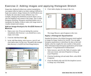
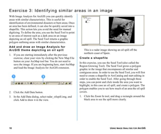
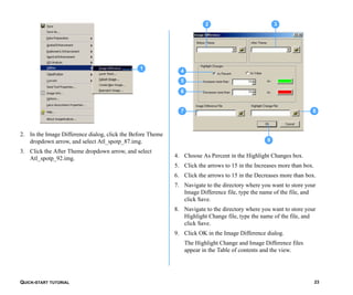
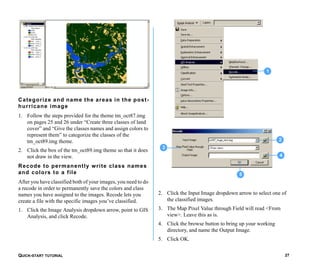
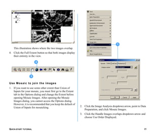
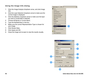
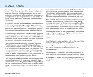
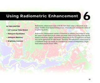
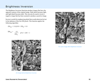
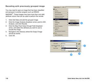
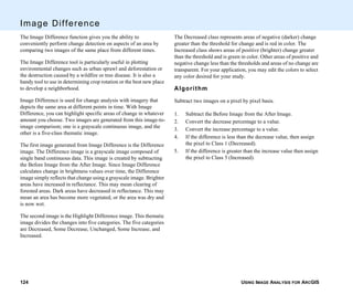
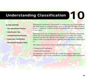
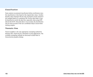
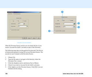
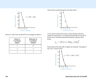
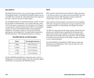
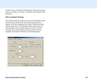
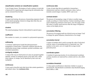
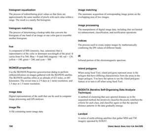
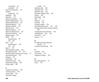
Maximum likelihood
Note: The maximum likelihood algorithm assumes that the
histograms of the bands of data have normal distributions. If this is
not the case, you may have better results with the minimum
distance decision rule.
The maximum likelihood decision rule is based on the probability
that a pixel belongs to a particular class. The basic equation
assumes that these probabilities are equal for all classes, and that
the input bands have normal distributions.
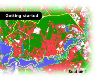
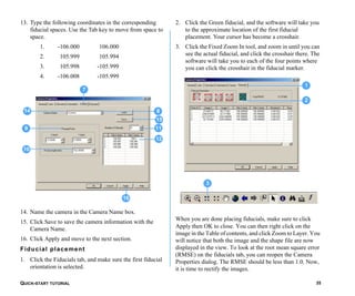
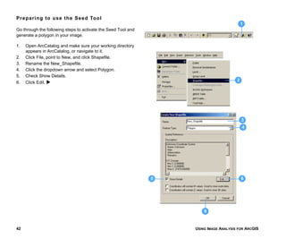
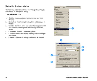
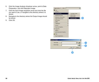
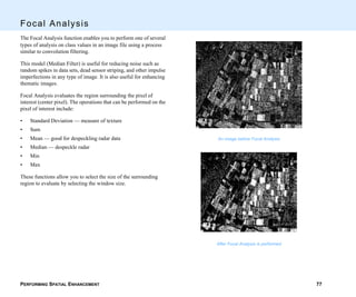
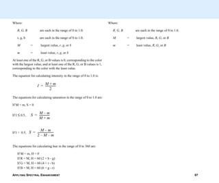
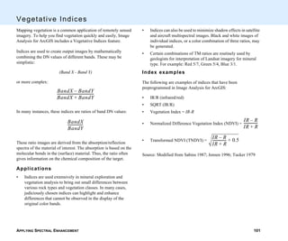
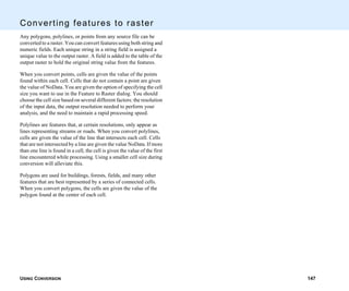
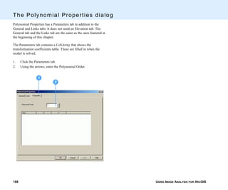
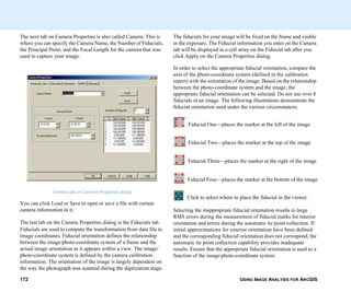
The Equation for the Maximum Likelihood/Bayesian Classifier is
as follows:
D ac( ) 0.5 Covc( )ln[ ]– 0.5 X Mc–( )T Covc
1–
( ) X Mc–( )[ ]–ln=
Where:
D = weighted distance (likelihood)
c = a particular class
X = the measurement vector of the candidate pixel
Mc = the mean vector of the sample of class c
ac = percent probability that any candidate pixel is
a member of class c (defaults to 1.0, or is
entered from a priori data)
Covc = the covariance matrix of the pixels in the
sample of class c
|Covc| = determinant of Covc (matrix algebra)
Covc-1 = inverse of Covc (matrix algebra)
ln = natural logarithm function
T = transposition function (matrix algebra)
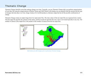
Mahalanobis distance
Note: The Mahalanobis distance algorithm assumes that the
histograms of the bands have normal distributions. If this is not the
case, you may have better results with the parallelepiped or
minimum distance decision rule, or by performing a first-pass
parallelepiped classification.
Mahalanobis distance is similar to minimum distance, except that
the covariance matrix is used in the equation. Variance and
covariance are figured in so that clusters that are highly varied lead
to similarly varied classes, and vice versa. For example, when
classifying urban areas—typically a class whose pixels vary
widely—correctly classified pixels may be farther from the mean
than those of a class for water, which is usually not a highly varied
class (Swain and Davis 1978).](https://image.slidesharecdn.com/erdas-imageanalysisforarcgis-160205132516/85/Erdas-image-analysis-for-arcgis-149-320.jpg)


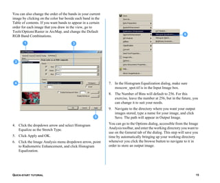
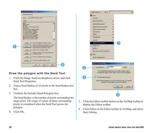
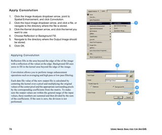
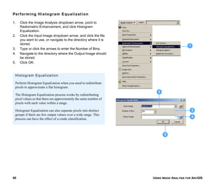
Here are the basic steps to start Image Analysis for ArcGIS: 1. Open ArcMap and add an image to your map. The image can be in a file geodatabase, personal geodatabase, or folder. 2. Click the Image Analysis button on the ArcMap toolbar to open the Image Analysis window. 3. In the Image Analysis window, click the Tools menu and select the tool you want to use, such as Histogram Stretch. 4. Configure the tool settings as needed and click OK to apply the tool to your image. 5. The results will display in your image layer in ArcMap. 6. Save your map document to preserve the changes made by the Image


